Abstract
Modern literature exhibits numerous centralized control approaches—event-based or model assisted—for tackling poor energy performance in buildings. Unfortunately, even novel building optimization and control (BOC) strategies commonly suffer from complexity and scalability issues as well as uncertain behavior as concerns large-scale building ecosystems—a fact that hinders their practical compatibility and broader applicability. Moreover, decentralized optimization and control approaches trying to resolve scalability and complexity issues have also been proposed in literature. Those approaches usually suffer from modeling issues, utilizing an analytically available formula for the overall performance index. Motivated by the complications in existing strategies for BOC applications, a novel, decentralized, optimization and control approach—referred to as Local for Global Parameterized Cognitive Adaptive Optimization (L4GPCAO)—has been extensively evaluated in a simulative environment, contrary to previous constrained real-life studies. The current study utilizes an elaborate simulative environment for evaluating the efficiency of L4GPCAO; extensive simulation tests exposed the efficiency of L4GPCAO compared to the already evaluated centralized optimization strategy (PCAO) and the commercial control strategy that is adopted in the BOC practice (common reference case). L4GPCAO achieved a quite similar performance in comparison to PCAO (with 25% less control parameters at a local scale), while both PCAO and L4GPCAO significantly outperformed the reference BOC practice.
1. Introduction
According to recent research, the building sector represent the largest energy consuming sector worldwide and so its conversion to affordable and eco-friendly structures portrays a major challenge for science and engineering [1]. Current policies and studies exhibit multiple energy-saving strategies aiming at an upgraded energy efficiency and also a lower carbon footprint in structures. Usually, these studies emphasize on the harsh-climate areas, where energy waste usually becomes severe due to extended heating and cooling demands, and therefore, the need for an improved energy saving plan becomes an absolute necessity [2,3,4,5,6,7]. Commonly encountered techniques—usually designated as passive or conventional—are focusing on the appropriate selection of structure materials and also the proper design of building’s envelope [8,9,10,11,12]. According to those practices, structures’ materials need to fulfill certain mechanical and physical requirements in order to comply with buildings’ characteristics for lowering internal energy wastage, increasing thermal storage ability and exploiting the available renewable energy sources [13,14,15]. However, passive renovation or retrofitting strategies usually result in a costly, disruptive and tedious procedure, hindering their wide applicability in the majority of building cases [16].
Contrary to passive approaches, advanced renovation techniques involve the Internet of Things (IoT) for automation, where the whole building structure is considered as an active ecosystem. Those active renovation approaches are focusing on a technologically advanced and cost-efficient automated approach, by dynamically orchestrating the active building elements for reducing the non-renewable energy usage while utilizing elaborate control strategies—such as heating, ventilating and air conditioning (HVAC) systems and renewable energy—through monitoring and automation schemes [17,18]. It should be underlined that according to modern literature, solitary passive approaches are not adequate enough to adequately exploit the energy saving potential. Therefore, a joint effort between active and passive strategies exposed a combined approach that can increase the energy saving potential [19,20]. As a result, modern building optimization and control (BOC) approaches promote diverse control strategies focusing on the balanced integration of both active and passive elements.
While those efforts may deliver a significant energy saving potential, they cannot produce a proper control optimization result due to their inflexible rule-based nature, their high building modelling complexity and the underlying dynamically changing factors (climate alterations, occupancy, envelopment deterioration, material aging, etc.). State-of-the-art control practices usually suffer from slow convergence rates, low stability and poor applicability (model-indented control approaches), exhibiting modeling oversimplifications (model-confided control approaches) as energy saving solutions. To this end, conventional practices usually encompass cost-ineffective, peculiar and time-wasting operations in order to create an elaborate building model, while, in most cases, representing insufficient performances due to model exaggerations and inaccuracies [21]. The problem becomes even more intense when BOC concerns large-scale, high-inertia buildings, due to the multiple reaction complexities that those structures represent in comparison with the conventional ones. In those cases, the BOC solution needs to act proactively in order to meet the building’s exceptional thermal criteria and to adequately exploit the elaborate structure-unique characteristics to produce a high-quality optimization result. Things become much more sophisticated when local energy generation (e.g., Renewable Energy Sources—RES) is also involved: the problem for optimized decision-making that preserves all the aforementioned context is being maximized, as control decisions need to deliver an integrated efficient strategy for exploiting renewable energy utilization.
1.1. Related Work and Novelty of the Paper
Conventional optimization strategies emphasizing the development of approximately effective agent-based BOC strategies in order to overcome the active restraints originated by systems of systems (SoS; system of systems is the viewing of various, scattered, unrelated, yet interacting systems in context as part of a wider, more complicated system) building ecosystem (BE) individual characteristics. According to literature, conventional optimization strategies can be classified into three main sets:
- Rule-based strategies that are mostly based on an ‘if-then’ type of control orders, in order to designate, for example, when to close off or turn on the equipment. Usually, a set of simplified control orders, determined by relevant experience, is applied. Unsuccessfully, strategies of this kind present a significant deficiency of adequate control and performance due to the fact that the control thresholds used are commonly empirical and do not exactly match the particular optimization control problem [22,23]. Actual building SoS-BEs are significantly overwhelmed by climate and tenancy particularities and certainly by behavioral alterations, caused by material changing or retrofitting operations. Moreover, manual manipulation of optimization control orders presents a burdensome activity since the peculiar interplay between the structures of SoS-BE characteristics is determined by an elaborate, nonlinear model [24,25,26].
- Model-driven strategies, where analytical or partial model information and its cost function is needed to utilize optimization and control approaches [27,28,29,30]. Such approaches, though, do not build the model from scratch but assume it as available, a practice that is usually not suitable considering the majority of real-life cases; advanced simulation approaches deliver cases based on predetermined simulation element templates (libraries) to structure the SoS-BE model, in a time adequate way. Besides manual modeling, black-box identification and machine learning methods [31,32,33,34,35] that assume the availability of elaborate historical datasets are also usually being utilized, extending the pre-application effort even more. Usually, modelling complexity issues are handled using general assumptions and modeling simplifications. In all modelling cases (manual or machine learning based), though, identifying a building SoS-BE is considered a tiresome and cost-inefficient process, imposing estimation errors that are circulated to the model-based BOC strategy.
- Agent-based techniques, where distributed computational load is of main importance. Unfortunately, agent-based topologies can achieve quite efficient behavior at the expense of higher data exchange rates or shared workspaces among each agent, a fact which limits their applicability only to smaller-scale control problems [36,37]. On the other hand, to minimize data exchange rates, several applications consider an isolated noncooperative optimization of local problems which share the same principal of minimizing locally-referring performance index [38,39,40]. Other approaches follow a double-layer architecture, where a central node is used to calculate global optimization indexes and constraints [41,42].
Following the paradigm of double-layer approaches, an advanced control optimization method considering buildings—identified as Local for Global Parameterized Cognitive Adaptive Optimization (L4GPCAO) [43,44]—has been specially formulated in order to effectively tackle the aforementioned implications in complicated BOC problems with uncertain dynamics. L4GPCAO exhibits the decentralized version of its centralized counterpart, PCAO, that has been extensively analyzed, revealing a remarkably high energy saving potential, even in real-life evaluations [45,46,47,48,49,50]. The L4GPCAO approach—similar to PCAO—demands nothing more than a single observable data point that summarizes the information of the entire performance to be periodically measured and shared de-centrally, unlike PCAO where all actions are executed centrally. The innovative characteristic of L4GPCAO is manifested from its agent-based character, where the overall centralized optimization problem is shattered into a set of several constituent parts. Each constituent part is determined by a dedicated agent, taking advantage of the decreased set of locally-available data for improving the global optimization goal. PCAO and L4GPCAO are independent considering the rational performance dynamics, demanding just one single evaluation of the holistic energy and discomfort performance periodically, while the overall objective function is considered observable but analytically unknown. In order to examine and evaluate its effectiveness, a holistically certified simulative building ecosystem, concerning the E.ON. Energy Research Centre of RWTH Aachen campus, is employed [51,52,53]. The primary target of this research effort is to measure and compare L4GPCAO’s performance towards the respective performance achieved by PCAO and by the existing market-oriented control strategy of the building. According to the comparisons, L4GPCAO’s ability to successfully shatter the complicated optimization control problem into several locally-driven ones proved successful, presenting a higher energy saving potential.
It should be underlined that the novelty of the presented study resides in the extended (simulative tests during different weather and seasonal conditions) verification tests conducted in an elaborated simulative environment as compared to previous studies of L4GPCAO, which did not extensively focus on the comparison of the thoroughly evaluated centralized (PCAO) and decentralized (L4GPCAO) methods [43,44]. The presented simulation results strongly underline the efficiency levels of the decentralized L4GPCAO as a locally-driven (i.e., local measurements are used for decentralized control feedback), minimal cross-system awareness (i.e., a single data point of global performance is shared across the system periodically), plug-n-play (i.e., readjustments of the optimization parameters are not required even, when different external conditions occur throughout the year) optimizer (see Section 3.5 for more details).
1.2. Test Case Building
The subject of this study consists of a dynamic model that is specifically structured in order to emulate the working behavior of the HVAC and control systems in the central building of E.ON Energy Research Center, located in Aachen, Germany [51,53,54]. Figure 1 portrays the front façade and the core energy supply system of the building. Its structure concerns a heated floor area of 1332 m2 while the main floor space is 892 m2. According to an aggregated long-term analysis, the heating demand is almost 30 kWh/m2 (5.3 kWh/m3) and the heated floor area demand is about 20 kWh/m2 per year.
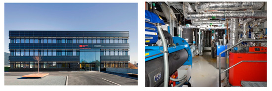
Figure 1.
E.ON. Energy research center: south façade mock-up view (left); central energy supply system (right) [55].
The envelope of the building includes wide glass openings, revealing the strong reliance of the internal thermal and visual conditions on the available (direct and indirect) sunlight levels, as illustrated in Figure 1. The energy design criteria for the particular building considered DIN EN 13779 [56] for thermal comfort, indoor air quality 2 (IDA 2), while indoor temperature is between 20 and 26 °C—a constraint that is necessary to be met for more than 50 h per year.
1.2.1. Building Ecosystem
The building is equipped with a complex energy conversion system supplying the building with thermal energy and electricity. Beside the non-renewable energy sources of gas and electricity, renewable energy sources and storages are available to operate the SoS-BE under an ecologically and economically high degree of quality. The distribution systems’ design was made by focusing on maximized load/demand coverage by renewable energy whilst the thermal comfort is preserved.
There are four distribution systems of different temperature levels. On the heating side, there is a high-temperature circuit containing gas-fired condensing boilers (as backup and for high-temperature applications) and a gas-fired combined heat and power system (CHP), which provides electricity, mainly for the heat pump. The turbo compressor-driven heat pump is meant to shift heat from the low-temperature heat circuit to the high-temperature cooling circuit. If the cooling loads are insufficient to cover heat demand by pure heat shifting, additional renewable energy can be used from the geothermal field, which is a 40-bore-hole heat exchanger in the building’s surrounding soil. Furthermore, a glycol cooler is available to ensure heat removal out of the system to the ambience if the energy balance is requiring that. The additional chiller supplies the low-temperature cooling circuits of server rooms and laboratories. A more detailed description of the energy concept of the building can be found in [51,57].
The building is used for research in building-application technology. Therefore, it is equipped with a high-standard energy supply system and a variety of HVAC equipment. However, the selected SoS-BE test-bed [52,58] represents three conventional conference rooms equipped as follows:
- Measured data/sensors: room temperature (T), room CO2 level, occupants’ presence contact (PS), window-opening sensor (WS), manual temperature dial (TD); energy consumption (EN) meters;
- Controlled devices/actuators: (i) air chiller (AC) systems for cooling the supply air from the central air handling unit individually for each room; and (ii) volume flow control (VFC) systems for adjusting the air flow rate individually for each room, separately, in supply and return air ducts.
- Non-actuatable: (i) concrete core activator (CCA) systems for base heating loads which are not eligible for real-time control due to building operation limitations and user comfort preservation purposes.
It should be noted that the controllable HVAC components (ACs and VFCs) are being supplied with energy by a combination of renewable and non-renewable sources integrated within the central energy system.
1.2.2. Simulation Tools and Libraries
The following paragraphs explain the arrangement of the simulation models of the building use case and the simulation framework with respect to the implementation of the Local4Global optimization algorithm. The dynamic behavior of the Thermal and Hydraulic system is simulated using Modelica, an object-oriented modelling language embedded in the commercial simulation environment called Dymola. For modelling purposes, the Modelica Standard library (URL: https://github.com/modelica/Modelica) as well as the AixLib Library (URL: https://github.com/RWTH-EBC/AixLib) are applied. AixLib portrays an open-source Modelica model library suitable for simulations that are being related with energy performance in building structures (https://github.com/RWTH-EBC/AixLib) [52].
The Control System is simulated using MATLAB/Simulink. Each room is controlled with a separate control algorithm and a higher level controller for coordinating the control parameters regarding the varying space sizes as a result of the folding walls between the rooms.
As a consequence of using these different simulation environments, there is a need for co-simulation. Therefore, TISC (http://www.tlk-thermo.com/en/software-products/tisc.html) is applied, transferring sensor values from Modelica to Simulink and control signals vice versa. Therefore, the control-related interrelations of both parts are modelled, even though the overall building structure has been modelled in separate simulation environments.
A scheme of the implementation platform of the Local4Global optimization algorithm is described in Figure 2 as well as in [52]. Equivalent to the real-life implementation of the algorithm in [44], the Local4Global optimization algorithm is processed simultaneously with the base control algorithm. The implementation uses the Local4Global optimization algorithm as a kind of ‘middleware’ optimizing the systems of systems building ecosystem (SoS-BE) operations by modifying the control signals received from Simulink before transmitting them to the actuators modelled in Modelica. This cycle is repeated in each communication step.
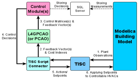
Figure 2.
Schematic illustration of the Local for Global Parameterized Cognitive Adaptive Optimization (L4GPCAO) implementation framework.
The rest of the paper is organized as follows: Section 2 presents the main ideas behind the proposed Local4Global PCAO methodology applied to BOC system design; Section 3 focuses on the specified building’s control objectives; in Section 4, the Local4Global PCAO BOC system design is extensively tested in numerous simulation scenarios and evaluated against the commercial reference control case used in practice and the centralized PCAO performance; and finally, Section 5 concludes the paper.
2. Local4Global PCAO for Control System Design
L4GPCAO is derived by discretizing the centralized optimization problem, which was considered for the Parameterized Cognitive Adaptive Optimization tool (PCAO) design, into several locally referring equivalent ones solved in a parallel manner. In reality, L4GPCAO coordinates several locally referring instances of PCAO where the distributed self-learning mechanisms are utilizing the overall performance instead of the local. The interested reader is referred to [46,59,60,61] for more details on PCAO. PCAO has already been tested and thoroughly evaluated within several simulations and real-life applications, presenting efficient behavior without the need for tedious pre-application effort and tuning [45,48,49,50].
Let us assume that the number of the locally driven L4GPCAO agents is set equal to while is the overall performance index considered; then, the algorithmic execution of L4GPCAO—against the respective one for PCAO—is explained below in a nutshell, with the following steps (see, also, Figure 3 and Figure 4):
| Step | PCAO | L4GPCAO |
| 1 | Initialize the central control matrix to be semi-definite positive between e1 and e2 eigenvalues (where e2 > e1 > 0) and define a scalar time-decaying continuous function a(t) to be used as the constantly decaying exploration radius for the generated central candidates considered in Step 4. | Initialize all N local control matrices to be semi-definite positive between e1 and e2 eigenvalues (where e2 > e1 > 0) and define a scalar time-decaying continuous function a(t) to be used as the constantly decaying exploration radius for the generated local candidates considered in Step 4. |
| 2 | Define the update Th period and apply the current control matrix for a whole update period. At the end of the period, calculate the overall performance index (see Appendix A.2.). | Define the update Th period and apply the current control matrices to the referring constituent plants/sub-systems for a whole update period. At the end of the period, calculate the overall performance index (see Appendix A.2.) and distribute it to all local constituent L4GPCAO agents. |
| 3 | Train a central linear-in-parameters estimator using the calculated values and the respective central control matrices as the central regressor vector. | Train a linear-in-parameters estimator in every constituent agent using the calculated values and the respective N local control matrices entries as the regressor vectors. |
| 4 | Generate a randomly perturbed by a(t) version of the applied central control matrix, using it as the perturbation center and the value of the time-decaying function defined in Step 1 as the exploration radius. | Generate randomly perturbed by a(t) versions of each locally applied control matrix, using them as the perturbation centers and the value of the time-decaying function defined in Step 1 as the exploration radius. |
| 5 | Estimate the performance of all generated central candidates from Step 4 using the respective central linear-in-parameters estimator from Step 3 and select the one expected to present the best overall performance. | Estimate the performance of all generated candidates from Step 4 using the respective local linear-in-parameters estimators from Step 3 and select the ones expected to present the best overall performance. |
| 6 | Set the selected matrix as the current one and GO TO Step 2 until performance convergence is achieved. | Set the selected matrices as the current ones and GO TO Step 2 until performance convergence is achieved. |
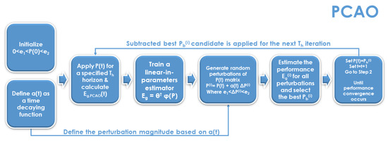
Figure 3.
PCAO algorithmic flowchart.
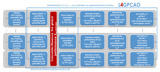
Figure 4.
L4GPCAO algorithmic flowchart.
The sequence of the L4GPCAO algorithm steps is illustrated herein. For additional information regarding the formulations and the underlying mathematical operations of the algorithm, the interested reader is referred to [43,44] and also to Appendix A.2..
3. Control Application Objectives
Climate control represents the largest segment of energy consumption in building structures, a fact that strongly depends on uncertain influences by user behavior and weather conditions. The simulation tests allow for evaluating different control strategies under the same conditions. The goal is to study L4GPCAO’s and PCAO’s potential of transforming the specific testbed into an energy-sustainable building while preserving indoor air and thermal comfort through intelligent HVAC use. As a key performance indicator, we focus on the non-renewable energy consumption (NREC). It represents the fraction of fossil energy used inside grids’ energy distribution for generating the net energy used for the building plant. This portion is assumed as 100% for every kWh gathered from the gas grid and 70% for each kWh taken from the electrical grid (it should be underlined that that selection of the energy share fractions is representing a scaling factor and does not modify the control optimization challenge evaluation analysis). The net energy consumption (NEC) is directly measured and used as the base for calculating NREC through an estimation of the actual energy supply system to ensure comparability with the results of the real life experiments [44]. In order to efficiently determine the NREC—stationed by the NEC—the fNR agent is utilized for the ratio of non-renewable energy in the net energy usage—presented in [44]; the control application is the NREC-driven regulation of the after cooler’s water valve (AC), supply and exhaust air volume flow (VFC), maintaining indoor air and thermal comfort.
This task is extremely demanding since it requires a sophisticated compound of quite extended and very short effect times of the HVAC system, a quite well-insulated structure increasing the effect of internal loads and solar radiation, and different, quite uncertain, unstable weather conditions. As a result, a quite complicated network of interlinked subsystems that exhibit different response times and constants determines the structures’ behavior under diverse situations and time intervals.
3.1. Operational Setup
PCAO and L4GPCAO were made MATLAB/Simulink-ready for the adequate execution of the simulation experiments. The finalized implementation workflow considered in the specific building application case is shown in Figure 5. Similar to the application deployment in [44], reconfigured instances of L4GPCAO and PCAO, in order to comply with the simulative application environment, e.g., TISC interfacing requirements and utilization of historical weather data were adopted. It should be noted that two asynchronous loops reflecting the actuation (control loop employing a simulation period of dt = 15 min) and the control recalibration (optimization loop employing a simulation period of Th = 4 × 24 = 96 h) schemas were implemented. The control loop is described using the dashed arrow, and additionally, the optimization loop is described with the solid arrow as Figure 5 portrays.
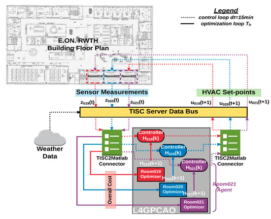
Figure 5.
L4GPCAO operational setup [HNN: control matrix strategy; uNN: control decisions vector; zNN: control feedback vector; xNN: stage variable vector; NN: room number indicator].
3.2. Optimization Setup
The simulative application allowed for replicated experiments considering the exact same external conditions (weather and occupancy conditions) in all three different control scenarios (reference building control (RBC), PCAO and L4GPCAO) to filter any discrepancies affected by them. In contrast to the application in [44] where this was not practically feasible, the optimization process workflow adopted considered an offline simulation schema for the tests (see, for example, Figure 6) where the control strategy is tuned for a certain simulation period by repeating the exact same model realization conditions (weather, occupancy) several times, while the applied control strategy is updated at the end of each repetition/iteration based on either PCAO (centralized control matrix) or L4GPCAO (constituent control matrices). The optimization process is active until performance convergence has been reached, i.e., the overall performance levels do not present significant changes between consequent simulation realizations/iterations.
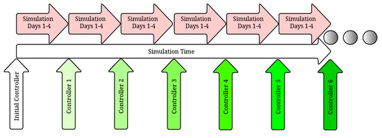
Figure 6.
Offline optimization setup.
3.3. Benchmark Control
In this particular research effort, we utilize the baseline case control approach and also PCAO control approach as the two comparison means against the performance of L4GPCAO. Two diverse control techniques were tried out and examined. Similar to the benchmark control case, the L4GPCAO and PCAO control strategies consider only the office working hours and days as the active control period from 8:00 until 17:00. For the simulation tests, the benchmark control strategy (base case) was based on real-life field observations—abbreviated, from now on, as reference building control (RBC)—since its commercial patent is protected by intellectual property and prototyping rights (i.e., it was considered as a black box). An RBC strategy that takes into account the simulation tests was planned and conducted, in the corresponding building management system (BMS), by the building designers and the commercial system contributor in a regular event-based procedure. That kind of technique utilizes a closed PID-based control loop that has been structured to respond to indoor temperature and CO2 variation in ACs and VFCs during heating periods in winter. Moreover, to avoid behavioral discrepancies of the plant itself among different control strategies’ application, the plant considered for evaluating the RBC strategy was the exact same one utilized also in the L4GPCAO and PCAO simulative tests, contrary to the limited real-life experiments case presented in [44].
3.4. Cost Function
Similar to the respective L4GPCAO real-life case study [44], to also avoid complexities during evaluation usually introduced when considering Fanger and PPD (predicted percentage of dissatisfied) metrics, the optimization criterion considered a simpler formulation that blends the non-renewable energy and the user discomfort factors as follows:
where 0 < w < 1 controls the significance of each respective factor in the cost function. Having in mind a harmonious, equally dependent optimization criterion among the non-renewable energy and discomfort, the w factor was set to 0.5. It should be mentioned that sophisticated research regarding the impact of different factor “w” selections is exists in literature [48,49].
The “Energyscore” factor corresponds to the total non-renewable energy consumption (NREC) (excessive energy requirement towards the possible renewable amount) normalized with the respective value “EnergyBscore” observed during the respective benchmark control tests (RBC case). The “DisComfortscore” was calculated using temperature and CO2 levels as the most significant indoor air (CO2) and thermal (temperature) discomfort-affecting variables—considering indoor humidity almost constant since no window openings are imposed in the simulative test scenarios—filtered to consider only the occupancy period. In order to fairly blend temperature and CO2 in a single evenly (f = 0.5) weighted index:
where
both are normalized to range between [0, 1], considering large-enough denominator values; respectively, Tmax = 28 °C in (3) and CO2max = 1100 ppm in (4). Similar to [44], the discomfort index is aligned with ASHRAE 55-2013 [62], EN 13779:2007 [56] (for indoor temperature acceptable value area) and ASHRAE 62.1-2013 [63] standards (for indoor CO2 acceptable value area), considering as an acceptable (non-penalizing) range for indoor temperature 21 and 24 °C in Equation (3) and 0 and 800 ppm for CO2 in Equation (4), respectively (see Equations (3) and (4) and Figure 7).
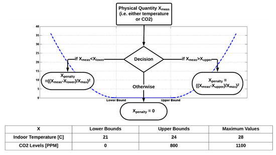
Figure 7.
Indoor temperature and CO2 penalization formulation.
As a result, both “Energyscore” and “DisComfortscore”, being unitless and ranging between [0, 1], contribute evenly (w = 0.5) to the total optimization index.
3.5. Closed-Loop Feedback Vector
For the closed-loop feedback vector formation, indoor measurements expressing the current condition of every constituent system along with the forecasted values of uncertain disturbance points (weather, occupancy) were considered. The prediction time interval that was elected was 3 h, short enough to guarantee low prediction/forecast faults. The feedback closed-loop vector structure, used in each optimization approach application, is shown in Table 1.

Table 1.
Feedback vector structure for PCAO and L4GPCAO application cases.
Moreover, after performing algebraic manipulations [43], based on the Hamilton–Jacobi–Bellman equation [64], the approximated optimal control formula can be written as follows:
where z represents the full column control feedback vector for the centralized and decentralized case as shown in the table above, x represents the respective localized or centralized state vectors, are the Jacobian matrices of z w.r.t. x, and is a constant matrix sized so as to filter the effect of the partial derivatives z(x), z(d), z(pd) w.r.t x. Finally, represents the square control matrices for each respective constituent system (L4GPCAO) and is the global one (PCAO).
| PCAO centralized | L4GPCAO decentralized |
By summarizing the number of the aforementioned feedback vector entries, the local measurements that were pointed out at every control time interval (dt = 15 min) (without the constant term) were 17. It should be mentioned that the parameters of the local squared control matrix for every constituent room are 18 × 18 = 324, i.e., when considering the (L4GPCAO) approach, every local agent contributes to the adjustment of 324 parameters. The number of the parameters that the centralized optimization strategy was adjusting raised to 36 × 36 = 1296—this number portrays the central squared control matrix parameters , and the number of pointed-out measurements that were collected centrally, without the constant term, is equal to 35.
It is obvious that in the L4GPCAO case, the centralized optimization problem (1296 parameters) turns into a computationally cheaper one (3 sub-problems × 324 parameters = 972 parameters overall). Additionally, in contrast to the centralized optimization strategy (35 data points that were necessary at a central node), the decentralized approach demand in data points was significantly lower and equal to 17 in every local sub-system, while only 1 data point is demanded centrally—as noted in Section 2—a fact that lowers the communication and infrastructure cost requirements for collecting data to a central node. That kind of diverse behaviour may be even greater when the scale of the relative building structure becomes even larger—for instance, when it concerns a larger amount of rooms, or even districts.
4. Simulation Experiments
This section provides details on the simulation experiments conducted for the test case building. Note that the number of sub-systems was considered equal to the number of the available rooms for tests, i.e., N = 3, and the optimization period was considered equal to four days, i.e., Th = 96 h, while the control period was set equal to dt = 15 min in all test cases. Moreover, the same values were adopted in all simulation cases for the optimization and control parameters as follows: , , for the boundary conditions of all semi-definite positive Pg, Pi matrices and , where as the time-decaying perturbation step formula. In all optimization cases, the control scheme was initialized with the exact same strategy, based on the defined lower and upper positive eigenvalue bounds (e1, e2), as also explained in [44]. At this point, it should be mentioned that the decision of e1, e2 values was defined so that the control decisions that resulted are mathematically acceptable (see Appendix A.2.) and realistic (scaled so as to vary between the defined operational control bounds). Finally, the occupancy schedule simulated is the same in all cases, emulating working hours between 9:00–18:00, following the same profile as the available control variables (e.g., see Figure A1c,d). In an attempt to maintain the readability, reduce the size and avoid too many details in the current document, the authors decided to provide a compact evaluation analysis of the presented simulation tests.
The simulation tests have been conducted using historical data collected in 2014 using an elaborate, validated building energy performance simulation (BEPS) [52] model for the building established in Modelica [65]. As already mentioned, several different simulation period cases (winter, spring, summer and autumn) have been considered, all with the same 4-working-day duration. The different climatic conditions, in terms of outdoor temperature and solar radiation, across the different seasonal periods are shown in Figure 8c. In addition, for performance comparison purposes, two different control and optimization topologies have been considered: centralized (PCAO) and decentralized (L4GPCAO). The centralized optimization counterpart (PCAO) tool was considered to provide a secondary benchmark point—besides the RBC module—reference control.
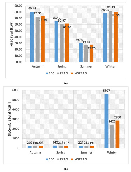
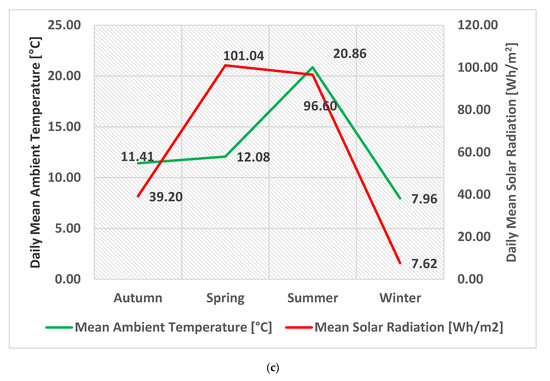
Figure 8.
Offline results summary: (a) Total non-renewable energy consumption (NREC) in all building optimization and control (BOC) and season cases (top). (b) Total DisComfort in all BOC and season cases (middle). (c) Average daily ambient temperature and average daily solar radiation for all season cases (bottom).
Results Analysis and Evaluation
As mentioned previously, the simulation horizon for the offline simulation tests was set equal to 4 days (Th = 96 h). The summarizing results from the three different control cases—(i) RBC, (ii) centralized PCAO and (iii) decentralized L4GPCAO—are presented in Figure 8. The respective absolute performance differences, in terms of NREC and DisComfort, observed between each building optimization and control (BOC) application case (centralized PCAO and decentralized L4GPCAO) and the reference building control (RBC) case are normalized over the latter (see Figure 9) to demonstrate the improvement percentages achieved respectively. It can be observed that in all L4GPCAO and PCAO cases, the total discomfort conditions are improved in comparison with the RBC reference control case. More specifically, L4GPCAO and PCAO improve the total performance by specifically minimizing both NREC consumption as well as indoor air and thermal discomfort index during autumn, spring and summer. A special occasion, though, is outlined during winter tests, where overall performance is improved again but by only significantly optimizing/minimizing the discomfort index through a small NREC increase. This dynamic implies that the RBC case was parameterized focusing on heavy winter heating periods when the energy demand for indoor climatizing is more intense. Note that the presented results for PCAO and L4GPCAO cases are referring to the ones generated after convergence was achieved (see the Subsection “Optimization Setup” above). For the PCAO case, performance convergence was achieved to a different centralized controller than the local controllers for each of the three constituent conference rooms in the L4GPCAO case.
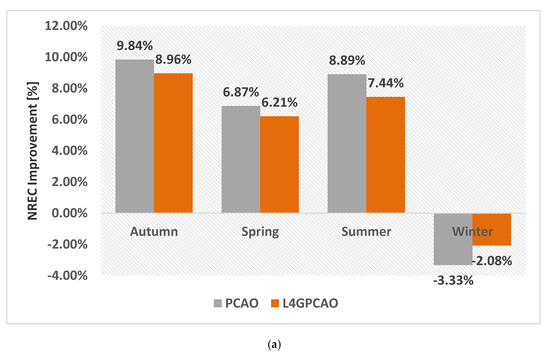
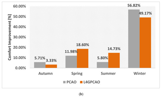
Figure 9.
Improvement percentages respect to the reference building control (RBC) case for: (a) total NREC in PCAO and L4GPCAO cases (top); (b) total comfort index in PCAO and L4GPCAO cases (bottom).
Both PCAO and L4GPCAO applications achieved significant NREC savings during the 4-day simulation period—while improving, slightly, the indoor comfort conditions—during the autumn, spring and summer test periods. On the other hand, the winter tests presented a higher NREC, when ambient temperature is always below 15 °C and the CCA systems are operated by the RBC strategy in heating mode. Both PCAO and L4GPCAO resulted in an increased NREC and AC usage (see Figure 9a) since indoor overheating combined with high CO2 levels would occur if the ACs were not used to cool down the indoor environment (see Figure 9b). It must be underlined that overheating and high CO2 concentration were both compensated, both by PCAO and L4GPCAO, which were responsible for controlling only the ACs and VFCs, while the RBC was responsible for controlling the CAs at all times. A more detailed analysis on the behavior of the three control strategies (PCAO, L4GPCAO and RBC) is also discussed in the Appendix A below to provide indicative insights during the autumn and winter tests.
Finally, the total average daily savings (in absolute numbers), presented in Table 2 below, could be translated into monetary values. The average daily NREC and comfort index values as well as the respective differences with the RBC cases have been included in Table 2. The average daily differences in the comfort index during the autumn, spring and summer periods suggest that quite similar indoor air and thermal conditions were achieved in all test cases. More specifically, the average total daily NREC reduction for the offline PCAO case during the autumn, spring and summer periods (when similar indoor conditions to the RBC case were achieved) is about 1.3 kWh/day and can be translated to 0.27 EUR/day by considering the EU-28 average electricity costs of 0.21 EUR/kWh (including tax) [66]. The respective NREC difference for the offline L4GPCAO case is about 1.1 kWh/day which can be translated to 0.23 EUR/day. On the other hand, offline PCAO and L4GPCAO consumed 0.7 kWh/day (i.e., 0.14 EUR/day) and 0.4 kWh/day (i.e., 0.08 EUR/day) more, respectively, during the winter period, while the indoor daily average comfort index was around 50% better.
Table 2.
Overall daily average savings and improvements of PCAO and L4GPCAO.
As expected, PCAO, which is a centralized optimization approach, slightly outperformed L4GPCAO, which employs several constituent reduced optimization parallel problems (i.e., a lower amount of information is required by each local optimizer). However, in essence, the L4GPCAO approach achieved comparable levels of improvement to its thoroughly verified and evaluated centralized counterpart PCAO (see Table 2 and Figure 9) within the same application horizon, by calibrating, in total, 1296 − 972 = 324, i.e., 25% less parameters (see Subsection “Closed-Loop Feedback Vector” above). Such a difference may become even more evident when the scale of the application becomes even larger, i.e., more rooms (or even buildings or districts) are involved.
5. Conclusions
Considering the construction and insulation features of the particular structure, PCAO and L4GPCAO strategies accomplished a noticeable improvement of the overall performance. The specified building case is considered a quite well-designed structure; wide-scale glass facades fostering a sunlight advantage, particularly efficient HVAC equipment (VFCs and ACs) and also advanced insulation materials that are adequate to significantly boost the energy saving potential of the structure. Additionally, the reference control case (RBC) is considered as one of the most trustworthy and effective commercial products that concerns the market of the building automation and management sector.
However, the PCAO and L4GPCAO decentralized BOC approaches achieved comparable improvements as far as non-renewable energy consumption is concerned, and also the indoor discomfort index, as compared to the RBC case. A special SoS-BE dynamic was revealed during the winter period tests, denoting that non-adaptive, on-the-fly optimization control is usually focused on certain extremely heavy occasions when high energy demand is expected. L4GPCAO, however, utilized 25% less parameters, narrowing the computational and data-transmission requirements of the overall SoS-BE optimization problem. Despite its decentralized nature, where a central BOC scheme and full knowledge of the system is absent at the local level, L4GPCAO achieved similar performance levels compared to the centralized one. Employing L4GPCAO renders the PCAO centralized optimization problem into a considerably lower computationally task. In cases where the scale of the plant becomes even larger, this optimization advantage may prove even greater—such as in larger building cases with a significantly greater number of rooms or even large building ecosystems or districts.
Author Contributions
Conceptualization, E.B.K.; Data curation, I.T.M. and R.S.; Formal analysis, I.T.M. and P.M.; Funding acquisition, E.B.K.; Investigation, I.T.M.; Project administration, D.M. and E.B.K.; Software, I.T.M., R.S. and T.S.; Writing—original draft, I.T.M. and R.S.; Writing—review & editing, I.T.M., R.S., P.M., T.S. and J.F. All authors have read and agreed to the published version of the manuscript.
Funding
The research leading to these results was partially funded by the European Commission FP7-ICT-2013.3.4, Advanced computing, Embedded Control Systems (Contract Number 611538) Local4Global—http://www.local4global-fp7.com/.
Conflicts of Interest
The authors declare no conflict of interest.
Nomenclature
| AC | Air Chiller | L4GPCAO | Local4Global PCAO |
| BCS | Base Case Scenario | MCIS | Monitoring, Control and Information System |
| BE | Building Ecosystem | MPC | Model Predictive Control |
| BEPS | Building Energy Performance Simulation | NEC | Net Energy Consumption |
| BOC | Building Optimization and Control | NREC | Non-renewable Energy Consumption |
| CCA | Concrete Core Activation | PCAO | Parameterized Cognitive Adaptive Optimization |
| CHP | Combined Heat and Power | RBC | Reference Building Control |
| CIP | Computer Investment Program | SoS | System of Systems |
| HJB | Hamilton–Jacobi–Bellman | VFC | Volume Flow Control |
| HVAC | Heating ventilating and air conditioning | VA,SUP | Air Volume Supply Rate |
| kWth | Kilowatt Thermal | VA,EXH | Air Volume Exhaust Rate |
Appendix A
Appendix A.1. Control Strategies Behavioral Analysis and Comparison
Since an elaborate discussion on the control behavior of all three strategies (PCAO, L4GPCAO and RBC) is out of the current study’s scope, this issue is briefly discussed herein in order to provide valuable yet indicative insights to the interested reader. To simplify their control behavior analysis further, the results presented originate from one single conference room. However, as depicted in Figure A1 and Figure A2 for both cases, both PCAO and L4GPCAO behaved almost identically, presenting quite minor control discrepancies which eventually resulted in their minor differences in NREC. Note that despite the fact that the AC valves were set equal to zero (eliminating the ACs’ cooling capability) outside of the occupancy period, for safety reasons, the respective VFCs were set to 0.3 (30%) in order to maintain the CO2 levels as low as possible while consuming a small amount of non-renewable energy due to the low availability of renewable energy during the same period of the day (afternoon and night).
During the autumn tests, both PCAO and L4GPCAO were able to utilize the AC-valves and the respective VFC flows less when compared with the RBC strategy, as shown by the control setpoints for all 4-day simulation periods in Figure A1c,d below. This phenomenon allowed to consume around 8–9% less total NREC (see Figure A1e) while achieving almost similar (i.e., around 3–5% better) comfort conditions (see Figure A1a,b,f).


Figure A1.
Autumn test results for Conference Room 020: (a) room temperature (°C); (b) room CO2 levels (ppm); (c) AC valve control (%); (d) VFC flaps control (%); (e) total NREC (kWh); (f) room DisComfort index; (g) ambient temperature (°C); (h) solar radiation (W/m2).
Figure A1.
Autumn test results for Conference Room 020: (a) room temperature (°C); (b) room CO2 levels (ppm); (c) AC valve control (%); (d) VFC flaps control (%); (e) total NREC (kWh); (f) room DisComfort index; (g) ambient temperature (°C); (h) solar radiation (W/m2).


During the winter tests, both PCAO and L4GPCAO were able to utilize the AC valves and the respective VFC flows more when compared with the RBC strategy, as shown by the control setpoints for all 4-day simulation periods, shown in Figure A2c,d below. This phenomenon allowed to consume around 2–3% more total NREC (see Figure A2e) while achieving significantly (i.e., over 50%) better discomfort conditions (see Figure A2f). Despite the fact that the RBC controller was designed to utilize only the CAs—while the ACs were disabled and VFCs were set close to zero to compensate with indoor air quality only without significantly affecting the indoor temperature (Figure A2c)—for heating purposes during winter, both PCAO and L4GPCAO were able to minimize the overheating (see the spikes over 23 °C in Figure A2a) as well as the unacceptably high CO2 levels (see the spikes over 1000 ppm in Figure A2b) caused by this strategy. Both optimized strategies decided to use a small portion of energy by setting the AC valves close to 10–15% (Figure A2c) and the VFCs to around 50–55% (Figure A2d) to compensate both with overheating (exceeding 23 °C) and high CO2 levels (exceeding 1000 ppm) during the occupancy period.


Figure A2.
Winter test results for Conference Room 020: (a) room temperature (°C); (b) room CO2 levels (ppm); (c) AC valve control (%); (d) VFC flaps control (%); (e) total NREC (kWh); (f) room DisComfort index; (g) ambient temperature (°C); (h) solar radiation (W/m2).
Figure A2.
Winter test results for Conference Room 020: (a) room temperature (°C); (b) room CO2 levels (ppm); (c) AC valve control (%); (d) VFC flaps control (%); (e) total NREC (kWh); (f) room DisComfort index; (g) ambient temperature (°C); (h) solar radiation (W/m2).


Appendix A.2. Optimization Problem Formulation
The classic control optimization problem of minimizing the total score (as formulated in Section 3.4) can be reformulated as calibrating the control parameters (for the centralized PCAO denoted with Pg; for the decentralized L4GPCAO denoted with Pi for i = 1, 2…, N) by minimizing the approximation error of each agent’s optimal cost-to-go function (denoted with for PCAO and for L4GPCAO) time derivative as derived by the Hamilton–Jacobi–Bellman equation [64] for the optimal strategy:
Note that the aforementioned formulation denotes that PCAO and L4GPCAO are solving equivalent but not strictly equal control optimization problems. Moreover, the parabolic formulation of the Bellman cost-to-go function was selected considering the imposed constraints of always being a positive and continuous function. As a consequence, all control parameter matrices P were defined to be semi-definite positive e1 < P < e2 (where 0 < e1 <e2 are both positive; being the boundary conditions for the eigenvalues of the P matrices defined) so that the respective cost-to-go functions V are always positive. The PCAO setup considers a centralized manner where all information (zg, Pg, Totalscore) is available while L4GPCAO is trying to minimize an equivalent index by utilizing the local measurements (zi); the local control parameters (Pi); and only the shared Totalscore global metric. As a result, each local agent is dedicated to minimizing the respective local performance index which blends the global Totalscore metric, thus employing a locally-driven (i.e., room-driven), coordinated, parallel optimization of an equivalent set of sub-problems.
References
- Ramesh, T.; Prakash, R.; Shukla, K. Life cycle energy analysis of buildings: An overview. Energy Build. 2010, 42, 1592–1600. [Google Scholar] [CrossRef]
- Wu, Z.; Wang, B.; Xia, X. Large-scale building energy efficiency retrofit: Concept, model and Control. Energy 2016, 109, 456–465. [Google Scholar] [CrossRef]
- Hestnes, A.G.; Kofoed, N.U. Effective retrofitting scenarios for energy efficiency and comfort: Results of the design and evaluation activities within the OFFICE project. Build. Environ. 2002, 37, 569–574. [Google Scholar] [CrossRef]
- Takebayashi, H.; Moriyama, M. Policy options for sustainable energy development. Build. Environ. 2007, 42, 2971–2979. [Google Scholar] [CrossRef]
- Casals, X.G. Analysis of building energy regulation and certification in Europe: Their role, limitations and differences. Energy Build. 2006, 38, 381–392. [Google Scholar] [CrossRef]
- Healy, J.D.; Clinch, J. Fuel poverty, thermal comfort and occupancy: Results of a national household-survey in Ireland. Appl. Energy 2002, 73, 329–343. [Google Scholar] [CrossRef]
- Frank, T. Climate change impacts on building heating and cooling energy demand in Switzerland. Energy Build. 2005, 37, 1175–1185. [Google Scholar] [CrossRef]
- Al-Homoud, M.S. Performance characteristics and practical applications of common building thermal insulation materials. Build. Environ. 2005, 40, 353–366. [Google Scholar] [CrossRef]
- Leckner, M.; Zmeureanu, R. Life cycle cost and energy analysis of a Net Zero Energy House with solar combisystem. Appl. Energy 2011, 88, 232–241. [Google Scholar] [CrossRef]
- Çakmanus, I. Renovation of existing office buildings in regard to energy economy: An example from Ankara, Turkey. Build. Environ. 2007, 42, 1348–1357. [Google Scholar] [CrossRef]
- Dascalaki, E.; Santamouris, M. On the potential of retrofitting scenarios for offices. Build. Environ. 2002, 37, 557–567. [Google Scholar] [CrossRef]
- Gustavsson, L.; Sathre, R. Variability in energy and carbon dioxide balances of wood and concrete building materials. Build. Environ. 2006, 41, 940–951. [Google Scholar] [CrossRef]
- Monahan, J.; Powell, J. An embodied carbon and energy analysis of modern methods of construction in housing: A case study using a lifecycle assessment framework. Energy Build. 2011, 43, 179–188. [Google Scholar] [CrossRef]
- Smeds, J.; Wall, M. Enhanced energy conservation in houses through high performance design. Energy Build. 2007, 39, 273–278. [Google Scholar] [CrossRef]
- Porta-Gándara, M.A.; Rubio, E.; Fernández, J.L.; Rubio-Royo, E. Economic feasibility of passive ambient comfort in Baja California dwellings. Build. Environ. 2002, 37, 993–1001. [Google Scholar] [CrossRef]
- Ibnmohammed, T.; Greenough, R.M.; Taylor, S.J.; Ozawameida, L.; Acquaye, A. Integrating economic considerations with operational and embodied emissions into a decision support system for the optimal ranking of building retrofit options. Build. Environ. 2014, 72, 82–101. [Google Scholar] [CrossRef]
- Ueno, T.; Sano, F.; Saeki, O.; Tsuji, K. Effectiveness of an energy-consumption information system on energy savings in residential houses based on monitored data. Appl. Energy 2006, 83, 166–183. [Google Scholar] [CrossRef]
- Piette, M.A.; Kinney, S.K.; Haves, P. Analysis of an information monitoring and diagnostic system to improve building operations. Energy Build. 2001, 33, 783–791. [Google Scholar] [CrossRef]
- Olofsson, T.; Mahlia, T.M.I. Modeling and simulation of the energy use in an occupied residential building in cold climate. Appl. Energy 2012, 91, 432–438. [Google Scholar] [CrossRef]
- Yang, L.; Yan, H.; Lam, J.C. Thermal comfort and building energy consumption implications—A review. Appl. Energy 2014, 115, 164–173. [Google Scholar] [CrossRef]
- Lehmann, B.; Dorer, V.; Gwerder, M.; Renggli, F.; Tödtli, J. Thermally activated building systems (TABS): Energy efficiency as a function, of control strategy, hydronic circuit topology and (cold) generation system. Appl. Energy 2011, 88, 180–191. [Google Scholar] [CrossRef]
- Doukas, H.; Patlitzianas, K.D.; Iatropoulos, K.; Psarras, J.E. Intelligent building energy management system using rule sets. Build. Environ. 2007, 42, 3562–3569. [Google Scholar] [CrossRef]
- Yao, Y.; Lian, Z.; Hou, Z.; Zhou, X. Optimal operation of a large cooling system based on an empirical model. Appl. Therm. Eng. 2004, 24, 2303–2321. [Google Scholar] [CrossRef]
- Alcalá, R.; Casillas, J.; Cordón, O.; González, A.; Herrera, F. A genetic rule weighting and selection process for fuzzy control of heating, ventilating and air conditioning systems. Eng. Appl. Artif. Intell. 2005, 18, 279–296. [Google Scholar] [CrossRef]
- Dong, Y.; Goh, A. An intelligent database for engineering applications. Artif. Intell. Eng. 1998, 12, 1–14. [Google Scholar] [CrossRef]
- Fong, K.; Hanby, V.; Chow, T. HVAC system optimization for energy management by evolutionary programming. Energy Build. 2006, 38, 220–231. [Google Scholar] [CrossRef]
- Wright, J.A.; Loosemore, H.A.; Farmani, R. Optimization of building thermal design and control by multi-criterion genetic algorithm. Energy Build. 2002, 34, 959–972. [Google Scholar] [CrossRef]
- Pourzeynali, S.; Lavasani, H.; Modarayi, A. Active control of high rise building structures using fuzzy logic and genetic algorithms. Eng. Struct. 2007, 29, 346–357. [Google Scholar] [CrossRef]
- Moon, J.; Jung, S.; Kim, Y.; Han, S. Comparative study of artificial intelligence-based building thermal control methods—Application of fuzzy, adaptive neuro-fuzzy inference system, and artificial neural network. Appl. Therm. Eng. 2011, 31, 2422–2429. [Google Scholar] [CrossRef]
- Liu, G.; Liu, M. A rapid calibration procedure and case study for simplified simulation models of commonly used HVAC systems. Build. Environ. 2011, 46, 409–420. [Google Scholar] [CrossRef]
- Youssef, A.; Caballero, N.; Aerts, J.-M. Model-based monitoring of occupant’s thermal state for adaptive HVAC predictive controlling. Processes 2019, 7, 720. [Google Scholar] [CrossRef]
- Dai, C.; Zhang, H.; Arens, E.; Lian, Z. Machine learning approaches to predict thermal demands using skin temperatures: Steady-state conditions. Build. Environ. 2017, 114, 1–10. [Google Scholar] [CrossRef]
- Ma, Y.; Borrelli, F.; Hencey, B.; Coffey, B.; Bengea, S.; Haves, P. Model predictive control for the operation of building cooling systems. IEEE Trans. Control Syst Technol. 2012, 20, 796–803. [Google Scholar]
- Oldewurtel, F.; Parisio, A.; Jones, C.N.; Gyalistras, D.; Gwerder, M.; Stauch, V.; Lehmann, B.; Morari, M. Use of model predictive control and weather forecasts for energy efficient building climate control. Energy Build. 2012, 45, 15–27. [Google Scholar] [CrossRef]
- Yang, I.-H.; Yeo, M.-S.; Kim, K.-W. Application of artificial neural network to predict the optimal start time for heating system in building. Energy Convers. Manag. 2003, 44, 2791–2809. [Google Scholar] [CrossRef]
- Gatsis, N.; Giannakis, G.B. Residential load control: Distributed scheduling and convergence with lost AMI messages. IEEE Trans. Smart Grid 2012, 3, 770–786. [Google Scholar] [CrossRef]
- Wang, X.; Yang, K. Economic load dispatch of renewable energy-based power systems with high penetration of large-scale hydropower station based on multi-agent glowworm swarm optimization. Energy Strategy Rev. 2019, 26, 100425. [Google Scholar] [CrossRef]
- Ma, K.; Hu, G.; Spanos, C. Distributed energy consumption control via real-time pricing feedback in smart grid. IEEE Trans. Control Syst. Technol. 2014, 22, 1907–1914. [Google Scholar] [CrossRef]
- Ma, Z.; Callaway, D.S.; Hiskens, I.A. Decentralized charging control of large populations of plug-in electric vehicles. IEEE Trans. Control Syst. Technol. 2013, 21, 67–78. [Google Scholar] [CrossRef]
- Liu, Z.; Chen, X.; Xu, X.; Guan, X. A decentralized optimization method for energy saving of HVAC systems. In Proceedings of the 2013 IEEE International Conference on Automation Science and Engineering (CASE), Madison, WI, USA, 17–20 August 2013; pp. 225–230. [Google Scholar]
- Ioli, D.; Deori, L.; Falsone, A.; Prandini, M. A two-layer decentralized approach to the optimal energy management of a building district with a shared thermal storage. IFAC Pap. 2017, 50, 8844–8849. [Google Scholar] [CrossRef]
- Gruber, J.K.; Prodanovic, M. Two-stage optimization for building energy management. Energy Procedia 2014, 62, 346–354. [Google Scholar] [CrossRef][Green Version]
- Kosmatopoulos, E.B.; Michailidis, I.; Korkas, C.D.; Ravanis, C. Local4Global adaptive optimization and control for system-of-systems. In Proceedings of the 2015 European Control Conference (ECC), Linz, Austria, 15–17 July 2015; pp. 3536–3541. [Google Scholar]
- Michailidis, I.T.; Schild, T.P.; Sangi, R.; Michailidis, P.; Korkas, C.D.; Fütterer, J.; Müller, D.; Kosmatopoulos, E.B. Energy-efficient HVAC management using cooperative, self-trained, control agents: A real-life German building case study. Appl. Energy 2018, 211, 113–125. [Google Scholar] [CrossRef]
- Baldi, S.; Michailidis, I.; Jula, H.; Kosmatopoulos, E.B.; Ioannou, P.A. A “plug-n-play” computationally efficient approach for control design of large-scale nonlinear systems using co-simulation. IEEE Control Syst. Mag. 2013, 34, 436–441. [Google Scholar] [CrossRef]
- Baldi, S.; Michailidis, I.; Ravanis, C.; Kosmatopoulos, E. Model-based and model-free ”Plug-n-Play” building energy efficient Control. Appl. Energy 2015, 154, 829–841. [Google Scholar]
- Baldi, S.; Michailidis, I.; Ntampasi, V.; Kosmatopoulos, E.B.; Papamichail, I.; Papageorgiou, M. Simulation-based synthesis for approximately optimal urban traffic light management. In Proceedings of the 2015 American Control Conference (ACC), Chicago, IL, USA, 1–3 July 2015; pp. 868–873. [Google Scholar]
- Michailidis, I.T.; Baldi, S.; Pichler, M.F.; Kosmatopoulos, E.B.; Rodríguez-Santiago, J. Proactive control for solar energy exploitation: A german high-inertia building case study. Appl. Energy 2015, 155, 409–420. [Google Scholar] [CrossRef]
- Michailidis, I.; Korkas, C.D.; Kosmatopoulos, E.B.; Nassie, E. Automated control calibration exploiting exogenous environment energy: An Israeli commercial building case study. Energy Build. 2016, 128, 473–483. [Google Scholar] [CrossRef]
- Michailidis, I.; Michailidis, P.; Rizos, A.; Korkas, C.D.; Kosmatopoulos, E.B. Automatically fine-tuned speed control system for fuel and travel-time efficiency: A microscopic simulation case study. In Proceedings of the 2017 25th Mediterranean Conference on Control and Automation (MED), Valletta, Malta, 3–6 July 2017; pp. 915–920. [Google Scholar]
- Sangi, R.; Baranski, M.; Oltmanns, J.; Streblow, R.; Muller, D. Modeling and simulation of the heating circuit of a multi-functional building. Energy Build. 2016, 110, 13–22. [Google Scholar] [CrossRef]
- Sangi, R.; Schild, T.P.; Daum, M.; Fütterer, J.; Streblow, R.; Müller, D.; Michailidis, I.; Kosmatopoulos, E. Simulation-based implementation and evaluation of a system of systems optimization algorithm in a building control system. In Proceedings of the 2016 24th Mediterranean Conference on Control and Automation (MED), Athens, Greece, 21–24 June 2016; pp. 1296–1301. [Google Scholar]
- Sangi, R.; Fuetterer, A.K.J.; Müller, D. A linear model predictive control for advanced building energy systems. In Proceedings of the 2017 25th Mediterranean Conference on Control and Automation (MED), Valletta, Malta, 3–6 July 2017; pp. 496–501. [Google Scholar]
- Sangi, R.; Müller, D. A novel hybrid agent-based model predictive control for advanced building energy systems. Energy Convers. Manag. 2018, 178, 415–427. [Google Scholar] [CrossRef]
- Sangi, R. Development of Exergy-Based Control Strategies for Building Energy Systems; RWTH Aachen University: Aachen, Germany, 2018. [Google Scholar]
- Beuth Verlag, DIN-EN-13779. Ventilation for Non-Residential Buildings—Performance Requirements for Ventilation and Room-Conditioning Systems; German Institute for Standardization: Berlin, Germany, 2007. [Google Scholar]
- Futterer, J.; Constantin, A.; A Schmidt, M.; Streblow, R.; Muller, D.; Kosmatopoulos, E.B. A multifunctional demonstration bench for advanced control research in buildings monitoring, control, and interface system. In Proceedings of the IECON 2013 39th Annual Conference of the IEEE Industrial Electronics Society, Vienna, Austria, 10–13 November 2013; pp. 5696–5701. [Google Scholar]
- Schild, T.P.; Fütterer, J.; Sangi, R.; Streblow, R.; Müller, D. System of Systems theory as a new perspective on building Control. In Proceedings of the 2015 23rd Mediterranean Conference on Control and Automation (MED), Torremolinos, Spain, 16–19 June 2015; pp. 783–788. [Google Scholar]
- Michailidis, I.; Baldi, S.; Kosmatopoulos, E.B.; Ioannou, P.A. Adaptive Optimal Control for Large-Scale Nonlinear Systems. IEEE Trans. Autom. Control 2017, 62, 5567–5577. [Google Scholar] [CrossRef]
- Kosmatopoulos, E.B.; Kouvelas, A. Large Scale Nonlinear Control System Fine-Tuning Through Learning. IEEE Trans. Neural Netw. 2009, 20, 1009–1023. [Google Scholar] [CrossRef][Green Version]
- Kosmatopoulos, E.B. An adaptive optimization scheme with satisfactory transient performance. Automatica 2009, 45, 716–723. [Google Scholar] [CrossRef]
- American National Standards Institute (ANSI), ASHRAE/ANSI-55-2013. Thermal Environmental Conditions for Human Occupancy; ANSI: New York, NY, USA, 2014; ISSN 1041-2336. [Google Scholar]
- American National Standards Institute (ANSI), ASHRAE/ANSI-62.1. Ventilation for Acceptable Indoor Air Quality; ANSI: New York, NY, USA, 2019; ISSN 1041-2336. [Google Scholar]
- Hannes, R.; Thomas, S.; del Luigi, R. Approximate optimal control by inverse CLF approach. IFAC Pap. 2015, 48, 286–291. [Google Scholar]
- Elmqvist, H. Modelica Evolution—From My Perspective; Linkoping University Electronic Press: Linköping, Sweden, 2014; Volume 96, pp. 17–26. [Google Scholar]
- Eurostat. Europe in Figures—Eurostat Yearbook. 2017. Available online: http://ec.europa.eu/eurostat/statistics-explained/index.php/Energy_price_statistics (accessed on 7 May 2019).


Publisher’s Note: MDPI stays neutral with regard to jurisdictional claims in published maps and institutional affiliations. |
© 2020 by the authors. Licensee MDPI, Basel, Switzerland. This article is an open access article distributed under the terms and conditions of the Creative Commons Attribution (CC BY) license (http://creativecommons.org/licenses/by/4.0/).