Exergy Evaluation of a Water Distribution System

Abstract

The water supply system is one of the most important elements in a city. Currently, many cities struggle with a water deficit problem. Water is a commonly available resource and constitutes the majority of land cover; however, its quality, in many cases, makes it impossible to use as drinking water. To treat and distribute water, it is necessary to supply a certain amount of energy to the system. An important goal of water utility operators is to assess the energy efficiency of the processes and components. Energy assessments are usually limited to the calculation of energy dissipation (sometimes called “energy loss”). From a physical point of view, the formulation of “energy loss” is incorrect; energy in water transport systems is not consumed but only transformed (dissipated) into other, less usable forms. In the water supply process, the quality of energy—exergy (ability to convert into another form)—is consumed; hence, a new evaluation approach is needed. The motivation for this study was the fact that there are no tools for exergy evaluation of water distribution systems. A model of the exergy balances for a water distribution system was proposed, which was tested for the selected case studies of a water supply system and a water treatment station. The tool developed allows us to identify the places with the highest exergy destructions. In the analysed case studies, the highest exergy destruction results from excess pressure (3939 kWh in a water supply system and 1082 kWh in a water treatment plant). The exergy analysis is more accurate for assessing the system compared to the commonly used energy-based methods. The result can be used for assessing and planning water supply system modernisation.

1. Introduction

For the process of abstraction, treatment, and distribution of water, some amount of energy should be delivered to initiate chemical and physical transformation. Numerous methods of assessing water supply systems have been presented in the literature. A review on energy-based methods of water supply system assessment has previously been published by Bylka and Mróz [1]. Energy assessment methods of water supply systems are usually based on physical and mathematical descriptions of energy transformation. Models of energy transformation in the water supply (known as energy balance) have been previously developed [2,3,4,5,6]. The main goal of performing energy balance assessments is to calculate the energy dissipation in each part of the water supply system. From a physical point of view, the phrase “energy loss” is incorrect. In a water transport system, energy is not consumed but only transformed (dissipated) into other, less usable forms [7,8,9,10]. The indicator that allows the assessment of the ability of energy to change is exergy. According to the definition, exergy is “the amount of work obtainable when some matter is brought to a state of thermodynamic equilibrium with the common components of its surrounding nature by means of reversible processes, involving interaction only with the above-mentioned components of nature” [11]. The exergy approach is well known in industrial and commercial energy system analyses [12]. Many exergy models have been developed to describe processes in which large amounts of energy are transformed, such as heating, cooling, and energy production Exergy has also been used to describe drying, distillation, renewable energy, biogas, medicine, and aerospace processes [13,14,15,16,17].

Exergy analysis has not been widely used for describing processes in water supply systems, and there are only a few publications regarding exergy descriptions in this type of system. The second law of thermodynamics has been used to describe the desalination process using reverse osmosis [18,19,20], to perform an economic analysis of the water treatment process [21], and to compare various water treatment technologies [22]. Detailed descriptions of the exergy model have been presented for the ultra-pure water production process [23]. Exergy-based methods have also been used to assess the quality of surface water [24] and analyse the energy transformations of groundwater intake [25]. Furthermore, exergy analysis has been used to describe municipal wastewater treatment processes [26,27,28,29,30].

Previous analyses [1] have shown that there is a lack of exergy transformation models for the entire water supply system. A literature review showed that the currently used methods are based only on the first law of thermodynamics. The main aim of this study is to present a new method of energy assessment for water supply systems based on exergy and includes both the first and second law of thermodynamics. The developed model was implemented in the QGIS software as a set of Python scripts and can be used to analyse any water supply system. This allows a better understanding and evaluation of the network processes. This assessment is the basis for developing better tools for planning system modernisation.

2. Methods of Evaluation

Energy transformation in water supply systems accompanies all the process components, including water intake, water treatment stations, water distribution systems, and water pumping stations. Energy transformation can be caused by different factors, such as chemical reactions, heat exchange, current flow, hydraulic friction, mechanic friction, and diffusion. The main goal of exergy analysis is to determine exergy destruction, which is caused by the increase in entropy as quantitatively described by the Guy–Stodola law shown in Equation (1):

$$\delta \dot{\mathrm{B}}={\mathrm{T}}_0{\dot{\mathrm{S}}}_{\mathrm{gen}}$$

(1)

where $\delta \dot{\mathrm{B}}$ is the rate of the internal exergy destruction of a thermodynamic system in an infinitely short time dτ [W], ${\mathrm{T}}_0$ is the reference temperature [K], and ${\dot{\mathrm{S}}}_{\mathrm{gen}}$ is the rate of total increase in entropy of a thermodynamic system in an infinitely short time dτ, [W*K-1].

The exergy balance can be expressed as:

$${\dot{\mathrm{B}}}_{\mathrm{in}}=\delta \dot{\mathrm{B}}+{\dot{\mathrm{B}}}_{\mathrm{use}}+\delta {\dot{\mathrm{B}}}_{\mathrm{ext}}+\Delta {\dot{\mathrm{B}}}_{\mathrm{HS}}+\delta {\dot{\mathrm{B}}}_{\mathrm{u}}$$

(2)

where ${\dot{\mathrm{B}}}_{\mathrm{in}}$ is the rate of exergy change entering the control volume [W], $\mathsf{\delta }\dot{\mathrm{B}}$ is the rate of the internal exergy destructions [W], ${\dot{\mathrm{B}}}_{\mathrm{use}}$ is the rate of usable exergy change leaving the control volume [W], ${\mathsf{\delta }\dot{\mathrm{B}}}_{\mathrm{ext}}$ is the rate of external exergy destructions [W], $\Delta {\dot{\mathrm{B}}}_{\mathrm{HS}}$ is the rate of exergy change in an external heat source [W], and ${\mathsf{\delta }\dot{\mathrm{B}}}_{\mathrm{u}}$ is the rate of exergy change in an isolated system [W].

The exergy description for water streams was presented by Martínez-Gracia et al. [31]. The total specific exergy of a water stream depends on the temperature, pressure, chemical composition, concentration of dissolved substances, and the speed and height of the water stream in relation to the reference level. The total specific exergy of the water stream can be calculated as follows:

$${\mathrm{b}}_{{\mathrm{H}}_2\mathrm{O}}={\mathrm{b}}_{\mathrm{t}}+{\mathrm{b}}_{\mathrm{mech}}+{\mathrm{b}}_{\mathrm{chem}}+{\mathrm{b}}_{\mathrm{con}}+{\mathrm{b}}_{\mathrm{k}}+{\mathrm{b}}_{\mathrm{pot}}$$

(3)

where ${\mathrm{b}}_{\mathrm{t}}$ is the thermal exergy [J], ${\mathrm{b}}_{\mathrm{mech}}$ is the mechanical exergy [J], ${\mathrm{b}}_{\mathrm{chem}}$ is the chemical exergy [J], ${\mathrm{b}}_{\mathrm{con}}$ is the exergy of concentration [J], ${\mathrm{b}}_{\mathrm{k}}$ is the kinetic exergy [J], and ${\mathrm{b}}_{\mathrm{pot}}$ is the potential exergy [J].

The chemical exergy depends on the chemical composition of the substance. Because the chemical exergy change in a water distribution system is exceptionally low, it is possible to neglect this value in technical calculations. After the assumption that the water temperature does not change during the supply, thermal exergy changes can also be omitted. In pipes in water supply systems, the flow velocity is typically low. Hence, the kinetic exergy of the water flow can be neglected in technical analyses.

A developed exergy model of a water supply system should include analyses of mechanical and potential exergy transformation. The specific mechanical exergy can be calculated using Equation (4):

$${\mathrm{b}}_{\mathrm{mech}}={\mathrm{v}}_{{\mathrm{H}}_2\mathrm{O}}(\mathrm{p}-{\mathrm{p}}_0)$$

(4)

where ${\mathrm{v}}_{{\mathrm{H}}_2\mathrm{O}}$ is the specific volume of water [m³/kg], p is the water pressure in pipes [Pa], and p₀ is the reference pressure [Pa].

The specific potential exergy of water can be calculated as follows:

$${\mathrm{b}}_{\mathrm{pot}}= \mathrm{g}(\mathrm{z}-{\mathrm{z}}_0)$$

(5)

where z is the height [m] and z₀ is the reference height [m].

The rate of exergy can be calculated as follows:

$${\dot{\mathrm{B}}}_{{\mathrm{H}}_2\mathrm{O}}={\mathrm{b}}_{{\mathrm{H}}_2\mathrm{O}}\ast {\dot{\mathrm{m}}}_{{\mathrm{H}}_2\mathrm{O}}\ast {\mathrm{b}}_{{\mathrm{H}}_2\mathrm{O}}$$

(6)

where ${\dot{\mathrm{m}}}_{{\mathrm{H}}_2\mathrm{O}}$ is the mass flux of water [kg/s].

3. Exergy Model of a Water Supply System

Water supply systems consist of water intake, treatment stations, and distribution systems. A water supply system scheme is presented in Figure 1.

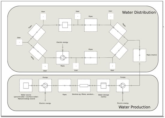
Figure 1. Scheme of a water supply system.

To develop an exergy balance for a water supply system, the hydraulic parameters of the network operation, including pressure in nodes and flow in pipes, are required. These values are obtained from mathematical models of the water supply system, which are based on the mass and energy conservation law. The water system is described by non-linear energy conservation equations (Bernoulli equations), linear mass conservation equations, and boundary conditions (pressure in water supply nodes—reservoir). Practically, systems of equations describing the flow and pressure in water supply networks are solved using computer programs. One of the best-known software packages for modelling water supply networks is Epanet, developed by the U.S. Environmental Protection Agency (US EPA) [32]. This model was adopted to develop exergy models of water supply systems. In the exergy models, six elements types are used, including the reservoir, pumps, pipes, nodes, valves, and tanks. Table 1 presents the sources of exergy destructions for each element in the water supply system.

Table 1. Source of exergy destructions in a water distribution system.

Types of Elements	Source of Exergy Destructions
Pumps	Hydraulic friction Electrical energy transformation to the kinetic and potential energy of water
Pipes	Hydraulic friction External exergy destructions (caused by leakage)
Nodes	Maintaining pressure higher than required
Valves	Hydraulic friction

Detailed exergy models for each element of the water supply system were developed using Equations (1)–(6). The exergy models are presented in Section 3.1, Section 3.2, Section 3.3, Section 3.4, Section 3.5, Section 3.6 and Section 3.7. In attachment 2, the list of used symbols is presented. The flow in a water distribution system is one-way and not circulated. Due to this fact, in this research the impact of the relation between the pressure inside a system and its environment was not taken into account [17,33].

3.1. Exergy Model for Reservoirs

A reservoir is constant, irresistible, and irrelevant to the outflow and headwater. Reservoirs are used to model water sources for water supply systems (e.g., streams, dams, or groundwater aquifers). From a mathematical point of view, reservoirs are used as boundary conditions.

The exergy model for a reservoir (Figure 2) can be calculated as follows:

$${\dot{\mathrm{B}}}_{\mathrm{r},\mathrm{out}}={\dot{\mathrm{m}}}_{{\mathrm{H}}_2\mathrm{O},\mathrm{r}}[{\mathrm{v}}_{{\mathrm{H}}_2\mathrm{O}}({\mathrm{p}}_{\mathrm{r}}-{\mathrm{p}}_0)+\mathrm{g}({\mathrm{H}}_{\mathrm{r}}-{\mathrm{H}}_0)]$$

(7)

where ${\dot{\mathrm{B}}}_{\mathrm{r},\mathrm{out} }$ is the rate of exergy outflow from the control volume CV_R [W], ${\dot{\mathrm{m}}}_{{\mathrm{H}}_2\mathrm{O},\mathrm{r}}$ is the mass flux of water outflow from the control volume CV_R [kg/s], ${\mathrm{v}}_{{\mathrm{H}}_2\mathrm{O}}$ is the specific volume of water [m³/kg], g is the gravity [m/s²], ${\mathrm{p}}_{\mathrm{r}}$ is the water pressure in the reservoir [Pa], and ${\mathrm{H}}_{\mathrm{r}}$ is the head water in the reservoir [m].

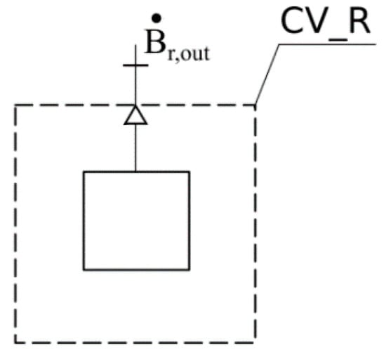
Figure 2. Exergy model for a reservoir.

3.2. Exergy Model for Pumps

Exergy destructions in pumps result from the imperfections in the conversion of electricity into potential and kinetic energy of water.

The exergy model for a pump (Figure 3) can be calculated as follows:

$${\dot{\mathrm{B}}}_{\mathrm{pump},\mathrm{in}}+{\mathrm{N}}_{\mathrm{p}}={\dot{\mathrm{B}}}_{\mathrm{pump},\mathrm{out}}+{ \mathsf{\delta }\dot{\mathrm{B}}}_{\mathrm{pump}}$$

(8)

where ${\dot{\mathrm{B}}}_{\mathrm{pump},\mathrm{in}}$ is the rate of exergy inflow to the control volume CV_PUMP (inlet pipe) [W], ${\dot{\mathrm{B}}}_{\mathrm{pump},\mathrm{out}}$ is the rate of exergy outflow from the control volume CV_PUMP (discharge pipe) [W], ${\mathrm{N}}_{\mathrm{p}}$ is the internal mechanical power required for the pump [W], and ${\mathsf{\delta }\dot{\mathrm{B}}}_{\mathrm{pump}}$ is the rate of the internal exergy destruction in the pump [W].

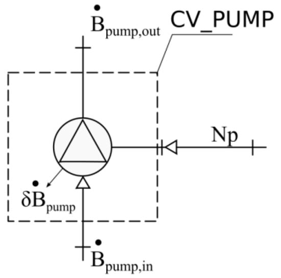
Figure 3. Exergy model for pumps.

The rate of exergy inflow to the control volume CV_PUMP can be calculated as follows:

$${\dot{\mathrm{B}}}_{\mathrm{pump},\mathrm{in}}={\dot{\mathrm{m}}}_{{\mathrm{H}}_2\mathrm{O},\mathrm{pump}} [{\mathrm{v}}_{{\mathrm{H}}_2\mathrm{O}}({\mathrm{p}}_{\mathrm{pump},\mathrm{in}}-{\mathrm{p}}_0)+\mathrm{g}({\mathrm{H}}_{\mathrm{pump},\mathrm{in}}-{\mathrm{H}}_0)]$$

(9)

where ${\dot{\mathrm{m}}}_{{\mathrm{H}}_2\mathrm{O},\mathrm{pump}}$ is the mass flux of water [kg/s], ${\mathrm{p}}_{\mathrm{pump},\mathrm{in}}$ is the water pressure inflow to the control volume CV_PUMP [Pa], and ${\mathrm{H}}_{\mathrm{pump},\mathrm{in}}$ is the elevation of pump inlet CV_PU [m].

The rate of exergy outflow from the control volume CV_PUMP can be calculated as follows:

$${\dot{\mathrm{B}}}_{\mathrm{pump},\mathrm{out}}={\dot{\mathrm{m}}}_{{\mathrm{H}}_2\mathrm{O},\mathrm{p}}[{\mathrm{v}}_{{\mathrm{H}}_2\mathrm{O}}({\mathrm{p}}_{\mathrm{ump},\mathrm{out}}-{\mathrm{p}}_0)+\mathrm{g}({\mathrm{H}}_{\mathrm{pump},\mathrm{out}}-{\mathrm{H}}_0)]$$

(10)

where ${\mathrm{p}}_{\mathrm{pump},\mathrm{out}}$ is the water pressure leaving the control volume CV_PUMP [Pa] and ${\mathrm{H}}_{\mathrm{pump},\mathrm{out}}$ is the elevation of pump outlet CV_PUMP [m].

The internal mechanical power required for the pump operation can be calculated as follows:

$${\mathrm{N}}_{\mathrm{p}}=\frac{{\dot{\mathrm{m}}}_{{\mathrm{H}}_2\mathrm{O}} [{\mathrm{v}}_{{\mathrm{H}}_2\mathrm{O}}({\mathrm{p}}_{\mathrm{pump},\mathrm{out}}-{\mathrm{p}}_{\mathrm{pump},\mathrm{in}})+\mathrm{g}({\mathrm{H}}_{\mathrm{pump},\mathrm{out}}-{\mathrm{H}}_{\mathrm{pump},\mathrm{in}})] }{\mathsf{\eta }}$$

(11)

where $\mathsf{\eta }$ is the pump efficiency (total).

The rate of the internal exergy destruction in the pump can be calculated as follows:

$${\mathrm{N}}_{\mathrm{p}}=\frac{{\dot{\mathrm{m}}}_{{\mathrm{H}}_2\mathrm{O}} [{\mathrm{v}}_{{\mathrm{H}}_2\mathrm{O}}({\mathrm{p}}_{\mathrm{pump},\mathrm{out}}-{\mathrm{p}}_{\mathrm{pump},\mathrm{in}})+\mathrm{g}({\mathrm{H}}_{\mathrm{pump},\mathrm{out}}-{\mathrm{H}}_{\mathrm{pump},\mathrm{in}})] }{\mathsf{\eta }}$$

(12)

3.3. Exergy Model for Pipes

In the pipes, exergy destructions are caused by friction head loss and by the water losses caused by pipe leaks. Most methods for modelling water supply networks assume the mass conservation law for pipes—the amount of water that flows into the pipe should be equal to the amount of water outflow from the pipe. Thus, it is not possible to include water losses in the exergy destruction model for pipes. Exergy destruction caused by leaks will be considered in the exergy model for nodes.

The exergy model for pipes (Figure 4) can be calculated as follows:

$${\dot{\mathrm{B}}}_{\mathrm{p},\mathrm{in}}={\dot{\mathrm{B}}}_{\mathrm{p},\mathrm{out}}+{ \mathsf{\delta }\dot{\mathrm{B}}}_{\mathrm{p}}$$

(13)

where ${\dot{\mathrm{B}}}_{\mathrm{p},\mathrm{in}}$ is the rate of exergy inflow to the control volume CV_P (in start node) [W], ${\dot{\mathrm{B}}}_{\mathrm{p},\mathrm{out}}$ is the rate of exergy outflow from the control volume CV_P (in end node) [W], and ${\mathsf{\delta }\dot{\mathrm{B}}}_{\mathrm{p}}$ is the rate of the internal exergy destruction in the pipes (caused by friction) [W].

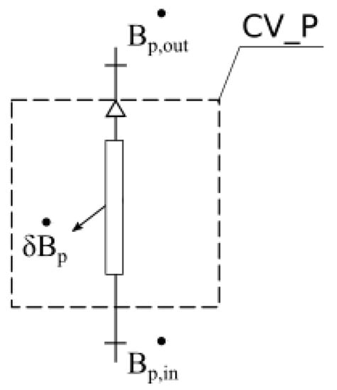
Figure 4. Exergy model for pipes.

The rate of exergy inflow to the control volume CV_P can be calculated as follows:

$${\dot{\mathrm{B}}}_{\mathrm{p},\mathrm{in}}={\dot{\mathrm{m}}}_{{\mathrm{H}}_2\mathrm{O},\mathrm{p}}[{\mathrm{v}}_{{\mathrm{H}}_2\mathrm{O}}({\mathrm{p}}_{\mathrm{p},\mathrm{in}}-{\mathrm{p}}_0)+\mathrm{g}({\mathrm{H}}_{\mathrm{p},\mathrm{in}}-{\mathrm{H}}_0)$$

(14)

where ${\dot{\mathrm{m}}}_{{\mathrm{H}}_2\mathrm{O},\mathrm{p}}$ is the mass flux of water flowing in pipes [kg/s], ${\mathrm{p}}_{\mathrm{p},\mathrm{in}}$ is the pressure in start node [Pa], and ${\mathrm{H}}_{\mathrm{p},\mathrm{in}}$ is the elevation of start node [m].

The rate of exergy outflow from the control volume CV_P can be calculated as follows:

$${\dot{\mathrm{B}}}_{\mathrm{p},\mathrm{out}}={\dot{\mathrm{m}}}_{{\mathrm{H}}_2\mathrm{O}} [{\mathrm{v}}_{{\mathrm{H}}_2\mathrm{O}}({\mathrm{p}}_{\mathrm{p},\mathrm{out}}-{\mathrm{p}}_0)+\mathrm{g}({\mathrm{H}}_{\mathrm{p},\mathrm{out}}-{\mathrm{H}}_0)]$$

(15)

where ${\mathrm{p}}_{\mathrm{p},\mathrm{out}}$ is the pressure in the end node [Pa] and ${\mathrm{H}}_{\mathrm{p},\mathrm{out}}$ is the elevation of the end node [m].

The rate of exergy outflow from the control volume CV_P can be calculated as follows:

$${\mathsf{\delta }\dot{\mathrm{B}}}_{\mathrm{p}}={\dot{\mathrm{m}}}_{{\mathrm{H}}_2\mathrm{O},\mathrm{in}}[{\mathrm{v}}_{{\mathrm{H}}_2\mathrm{O}}({\mathrm{p}}_{\mathrm{p},\mathrm{out}}-{\mathrm{p}}_{\mathrm{p},\mathrm{in}})- \mathrm{g}({\mathrm{H}}_{\mathrm{p},\mathrm{in}}-{\mathrm{H}}_{\mathrm{p},\mathrm{out}})]$$

(16)

where $({\mathrm{p}}_{\mathrm{p},\mathrm{out}}-{\mathrm{p}}_{\mathrm{p},\mathrm{in}})$ is the head loss caused by friction in pipes [Pa].

3.4. Exergy Model for Nodes

In water distribution system models, it is assumed that water is delivered to the node. The useful exergy of water is delivered with the mass of water consumed by the end-user. To supply water to all users, an appropriate network pressure should be maintained, which depends on building height, installation, and the required pressure at the draw-down point. The optimal solution, from the point of view of network operation, would be to maintain a water pressure equal to the minimum pressure. Because of the terrain and network characteristics, this is not possible in most cases. To maintain adequate pressure at the most unfavourable points in the network, excess pressure will be experienced by other parts of the water distribution system. However, maintaining a higher than required pressure causes exergy destruction. Network leaks will also cause exergy destructions in nodes. The value of the losses depends on many parameters, including the network age, level of maintenance, materials used, and pressure, among other factors. In the exergy model, the simplifying assumptions are that water losses are determined by the percentage loss indicator and are assigned to the node. Water losses are calculated during a water loss audit, as a value of the percentage of losses. In the exergy model, it is assumed that water loss does not depend on pressure and does not change during the day.

An exergy model for nodes (Figure 5) can be calculated as follows:

$${\dot{\mathrm{B}}}_{\mathrm{j},\mathrm{in}}={\dot{\mathrm{B}}}_{\mathrm{j},\mathrm{out}}+{\dot{\mathrm{B}}}_{\mathrm{use}}+{ \Delta \dot{\mathrm{B}}}_{\mathrm{loss}}+{\mathsf{\delta }\dot{\mathrm{B}}}_{\mathrm{exc}}$$

(17)

where ${\dot{\mathrm{B}}}_{\mathrm{j},\mathrm{in}}$ is the rate of exergy inflow to the control volume CV_J [W], ${\dot{\mathrm{B}}}_{\mathrm{j},\mathrm{out}}$ is the rate of exergy outflow from the control volume CV_J [W], ${\dot{\mathrm{B}}}_{\mathrm{use}}$ is the rate of usable exergy outflow from the control volume CV_J [W], ${\Delta \dot{\mathrm{B}}}_{\mathrm{loss}}$ is the rate of external exergy destructions, caused by a loss of water mass because of leakage from the control volume CV_J [W], and ${\mathsf{\delta }\dot{\mathrm{B}}}_{\mathrm{exc}}$ is the rate of internal exergy destructions caused by excess pressure in the node [W].

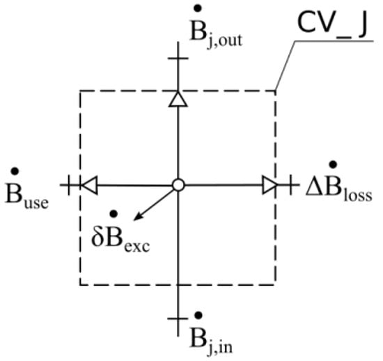
Figure 5. Exergy model for nodes.

The rate of exergy inflow to the control volume CV_J can be calculated as follows:

$${\dot{\mathrm{B}}}_{\mathrm{j},\mathrm{in}}={\dot{\mathrm{m}}}_{{\mathrm{H}}_2\mathrm{O},\mathrm{j},\mathrm{in}} [{\mathrm{v}}_{{\mathrm{H}}_2\mathrm{O}}({\mathrm{p}}_{\mathrm{j}}-{\mathrm{p}}_0)+\mathrm{g}({\mathrm{H}}_{\mathrm{j}}-{\mathrm{H}}_0)]$$

(18)

where ${\dot{\mathrm{m}}}_{{\mathrm{H}}_2\mathrm{O},\mathrm{j},\mathrm{in}}$ is the mass flux of water inflowing to the node [kg/s], ${\mathrm{p}}_{\mathrm{j}}$ is the pressure in the node [Pa], and ${\mathrm{H}}_{\mathrm{j}}$ is the nodes’ elevation [m].

The rate of usable exergy outflow from the control volume CV_J can be calculated as follows:

$${\dot{\mathrm{B}}}_{\mathrm{j},\mathrm{out}}={\dot{\mathrm{m}}}_{{\mathrm{H}}_2\mathrm{O},\mathrm{j},\mathrm{out}}[{\mathrm{v}}_{{\mathrm{H}}_2\mathrm{O}}({\mathrm{p}}_{\mathrm{j}}-{\mathrm{p}}_0)+\mathrm{g}({\mathrm{H}}_{\mathrm{j}}-{\mathrm{H}}_0)].$$

(19)

where ${\dot{\mathrm{m}}}_{{\mathrm{H}}_2\mathrm{O},\mathrm{j},\mathrm{out}}$ is the mass flux of water outflowing to the node [kg/s].

The rate of usable exergy outflow from the control volume CV_J (delivered to the user) can be calculated as follows:

$${\dot{\mathrm{B}}}_{\mathrm{use}}={\dot{\mathrm{m}}}_{{\mathrm{H}}_2\mathrm{O},\mathrm{j},\mathrm{use}} [{\mathrm{v}}_{{\mathrm{H}}_2\mathrm{O}}({\mathrm{p}}_{\mathrm{wym}}-{\mathrm{p}}_0)+\mathrm{g}({\mathrm{H}}_{\mathrm{j}}-{\mathrm{H}}_0)]$$

(20)

where ${\dot{\mathrm{m}}}_{{\mathrm{H}}_2\mathrm{O},\mathrm{j},\mathrm{use}}$ is the mass flux of water delivery to the user [kg/s] and ${\mathrm{p}}_{\mathrm{wym}}$ is the required pressure in the node [Pa].

The rate of external exergy destructions, caused by loss of water mass because of leakage from the control volume CV_J can be calculated as follows:

$${\Delta \dot{\mathrm{B}}}_{\mathrm{loss}}={\dot{\mathrm{m}}}_{{\mathrm{H}}_2\mathrm{O},\mathrm{j},\mathrm{loss}} [{\mathrm{v}}_{{\mathrm{H}}_2\mathrm{O}}({\mathrm{p}}_{\mathrm{j}}-{\mathrm{p}}_0)+\mathrm{g}({\mathrm{H}}_{\mathrm{j}}-{\mathrm{H}}_0)]$$

(21)

where ${\dot{\mathrm{m}}}_{{\mathrm{H}}_2\mathrm{O},\mathrm{j},\mathrm{loss}}$ is the mass flux of water losses because of leakage [kg/s]

The rate of internal exergy destructions caused by excess pressure in the node:

$${\mathsf{\delta }\dot{\mathrm{B}}}_{\mathrm{exc}}={\dot{\mathrm{m}}}_{{\mathrm{H}}_2\mathrm{O},\mathrm{j},\mathrm{use}} [{\mathrm{v}}_{{\mathrm{H}}_2\mathrm{O}}({\mathrm{p}}_{\mathrm{j}}-{\mathrm{p}}_{\mathrm{wym}})+\mathrm{g}({\mathrm{H}}_{\mathrm{j}}-{\mathrm{H}}_0)]$$

(22)

where ${\dot{\mathrm{m}}}_{{\mathrm{H}}_2\mathrm{O},\mathrm{j},\mathrm{exc}}$ is the mass flux of water delivered to the user [kg/s].

3.5. Exergy Model for Valves

The source of exergy destruction in valves is minor head loss. Using valves, any type of device (with known hydraulic characteristics) can be represented.

The exergy model for valves (Figure 6) can be calculated as follows:

$${\dot{\mathrm{B}}}_{\mathrm{v},\mathrm{in}}={\dot{\mathrm{B}}}_{\mathrm{v},\mathrm{out}}+{ \mathsf{\delta }\dot{\mathrm{B}}}_{\mathrm{v}}$$

(23)

where ${\dot{\mathrm{B}}}_{\mathrm{v},\mathrm{in}}$ is the rate of exergy inflow to the control volume CV_V [W], ${\dot{\mathrm{B}}}_{\mathrm{v},\mathrm{in}}$ is the rate of exergy outflow from the control volume CV_V [W], and ${\mathsf{\delta }\dot{\mathrm{B}}}_{\mathrm{v}}$ is the rate of internal exergy destruction in the control volume [W].

Figure 6. Exergy model for minor head loss (valves).

The rate of exergy inflow to the control volume CV_V can be calculated as follows:

$${\dot{\mathrm{B}}}_{\mathrm{v},\mathrm{in}}= [{\mathrm{v}}_{{\mathrm{H}}_2\mathrm{O}}({\mathrm{p}}_{\mathrm{v},\mathrm{in}}-{\mathrm{p}}_0)+\mathrm{g}({\mathrm{H}}_{\mathrm{v},\mathrm{in}}-{\mathrm{H}}_0)]{\dot{\mathrm{m}}}_{{\mathrm{H}}_2\mathrm{O},\mathrm{v}}$$

(24)

where ${\dot{\mathrm{m}}}_{{\mathrm{H}}_2\mathrm{O},\mathrm{v}}$ is the mass flux of water [kg/s], ${\mathrm{p}}_{\mathrm{v},\mathrm{in}}$ is the pressure of water inflow to the control volume CV_V [Pa], and ${\mathrm{H}}_{\mathrm{v},\mathrm{in}}$ is the inflow elevation CV_V [m].

The rate of exergy outflow from the control volume CV_V can be calculated as follows:

$${\dot{\mathrm{B}}}_{\mathrm{v},\mathrm{out}}={\dot{\mathrm{m}}}_{{\mathrm{H}}_2\mathrm{O},\mathrm{v}}[{\mathrm{v}}_{{\mathrm{H}}_2\mathrm{O}}({\mathrm{p}}_{\mathrm{v},\mathrm{out}}-{\mathrm{p}}_0)+\mathrm{g}({\mathrm{H}}_{\mathrm{v},\mathrm{out}}-{\mathrm{H}}_0)].$$

(25)

where ${\mathrm{p}}_{\mathrm{v},\mathrm{out}}$ is the pressure of water outflow from the control volume CV_V [Pa] and ${\mathrm{H}}_{\mathrm{v},\mathrm{out}}$ is the outflow elevation CV_V [m].

Assuming that ${\mathrm{H}}_{\mathrm{v},\mathrm{in}}$ = ${\mathrm{H}}_{\mathrm{v},\mathrm{out}}$, the rate of internal exergy destruction in the control volume CV_V can be calculated as follows:

$${\mathsf{\delta }\dot{\mathrm{B}}}_{\mathrm{v}}={\dot{\mathrm{m}}}_{{\mathrm{H}}_2\mathrm{O}}[{\mathrm{v}}_{{\mathrm{H}}_2\mathrm{O}}({\mathrm{p}}_{\mathrm{v},\mathrm{in}}-{\mathrm{p}}_{\mathrm{v},\mathrm{out}})]$$

(26)

where $({\mathrm{p}}_{\mathrm{v},\mathrm{in}}-{\mathrm{p}}_{\mathrm{v},\mathrm{out}})$ is the minor head loss [Pa].

3.6. Exergy Model for Tanks

Tanks are used in water supply networks, to compensate for unequal water demand during the day. Tanks store water mass and exergy and there is no exergy destruction in water tanks. Tanks should be included in the exergy balance because some of the exergies can be “magazined” in tanks at the end of analysis simulation time.

The exergy model for tanks (Figure 7) can be calculated as follows:

$${\dot{\mathrm{B}}}_{\mathrm{t},\mathrm{in}}={\dot{\mathrm{B}}}_{\mathrm{t},\mathrm{out}}+ \Delta {\dot{\mathrm{B}}}_{\mathrm{t}}+ \delta {\dot{\mathrm{B}}}_{\mathrm{t}}$$

(27)

where $\dot{{\mathrm{B}}_{\mathrm{t},\mathrm{in}}}$ is the rate of exergy inflow to the control volume CV_T [W], $\dot{{\mathrm{B}}_{\mathrm{t},\mathrm{out}}}$ is the rate of exergy outflow from the control volume CV_T [W], $\Delta {\dot{\mathrm{B}}}_{\mathrm{t}}$ represents the changes of exergy stored in control volume CV_T [W], and ${\mathsf{\delta }\dot{\mathrm{B}}}_{\mathrm{t}}$ is the rate of external exergy destruction from the control volume CV_T [W].

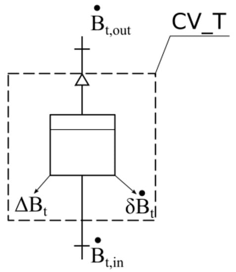
Figure 7. Exergy model for tanks.

Assuming that ${\mathsf{\delta }\dot{\mathrm{B}}}_{\mathrm{t}}$ = 0 (there is no water loss in the tanks), the rate of exergy inflow to the control volume CV_T can be calculated as follows:

$${\dot{\mathrm{B}}}_{\mathrm{t},\mathrm{in}}={\dot{\mathrm{m}}}_{{\mathrm{H}}_2\mathrm{O},\mathrm{t},\mathrm{in}} [{\mathrm{v}}_{{\mathrm{H}}_2\mathrm{O}}({\mathrm{p}}_{\mathrm{t}}-{\mathrm{p}}_0)+\mathrm{g}({\mathrm{H}}_{\mathrm{t}}-{\mathrm{H}}_0)]$$

(28)

where ${\dot{\mathrm{m}}}_{{\mathrm{H}}_2\mathrm{O},\mathrm{t},\mathrm{in}}$ is the mass flux of water inflowing to the tank [kg/s], ${\mathrm{p}}_{\mathrm{t}}$ is the water pressure in the tank [Pa], and ${\mathrm{H}}_{\mathrm{t}}$ is the water head in the tank [m].

The rate of exergy outflow from the control volume CV_P can be calculated as follows:

$${\dot{\mathrm{B}}}_{\mathrm{t},\mathrm{out}}={\dot{\mathrm{m}}}_{{\mathrm{H}}_2\mathrm{O},\mathrm{t},\mathrm{out}} [{\mathrm{v}}_{{\mathrm{H}}_2\mathrm{O}}({\mathrm{p}}_{\mathrm{t}}-{\mathrm{p}}_0)+\mathrm{g}({\mathrm{H}}_{\mathrm{t}}-{\mathrm{H}}_0)]$$

(29)

where ${\dot{\mathrm{m}}}_{{\mathrm{H}}_2\mathrm{O},\mathrm{t},\mathrm{out}}$ is the mass flux of water outflowing from the tank [kg/s].

Changes in exergy stored in the control volume CV_T can be calculated as follows:

$$\Delta {\dot{\mathrm{B}}}_{\mathrm{t}}=({\mathrm{m}}_{{\mathrm{H}}_2\mathrm{O},\mathrm{t},\mathrm{out}}-{\dot{\mathrm{m}}}_{{\mathrm{H}}_2\mathrm{O},\mathrm{t},\mathrm{in}})[{\mathrm{v}}_{{\mathrm{H}}_2\mathrm{O}}({\mathrm{p}}_{\mathrm{t}}-{\mathrm{p}}_0)+\mathrm{g}({\mathrm{H}}_{\mathrm{t}}-{\mathrm{H}}_0)$$

(30)

In the energy balance, $\Delta {\dot{\mathrm{B}}}_{\mathrm{tank}}$ can be:

• $\Delta {\dot{\mathrm{B}}}_{\mathrm{t}}=0$—water levels in the tank at the beginning and end of analysis are equal.
• $\Delta {\dot{\mathrm{B}}}_{\mathrm{t}}>0$—water level in the tank is higher at the end than at the start of analysis.
• $\Delta {\dot{\mathrm{B}}}_{\mathrm{t}}<0$—water level in the tank is lower at the end than at the start of analysis.

3.7. Exergy Model for Devices

In the water supply system (e.g., in treatment plants, intake), there are devices, such as aerators, filters, and nozzles, among others, in which physical exergy destructions are caused by the friction of the flow. Destruction of exergy can also result from other causes, such as diffusion, dissolution, and disposal of waste products (e.g., sludge), among others.

The general exergy model for devices (Figure 8) can be calculated as follows:

$${\displaystyle \sum }{\dot{B}}_{u,in}={\dot{B}}_{u,out}+{\displaystyle \sum }\delta {\dot{B}}_{u,w}+ {\displaystyle \sum }{\dot{B}}_{u,dis}.$$

(31)

where ${\displaystyle \sum }{\dot{\mathrm{B}}}_{\mathrm{u},\mathrm{in}}$ is the sum of the exergy rates of water and reagents inflow to the control volume CV_U, ${\dot{\mathrm{B}}}_{\mathrm{u},\mathrm{out}}$ is the sum of the exergy rates of water and reagents outflow from the control volume CV_U, ${\displaystyle \sum }{\mathsf{\delta }\dot{\mathrm{B}}}_{\mathrm{u},\mathrm{w}}$ is the sum of the exergy destructions rates of water and reagents in the control volume CV_U, and ${\displaystyle \sum }{\dot{\mathrm{B}}}_{\mathrm{u},\mathrm{dis}}$ is the sum of the exergy destructions rates of all waste products with positive useful exergy.

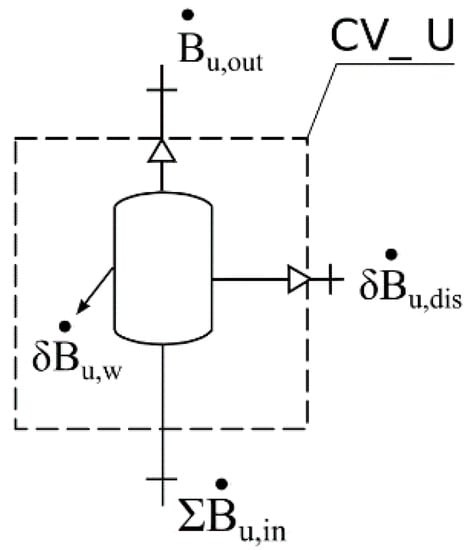
Figure 8. Exergy model for devices.

4. Case Studies

Two case studies are presented here: a water distribution network and a water treatment plant. Exergy balance was performed based on hydraulic modelling of each case using the Epanet software. For research purposes, computer tools for exergy calculations were developed in the QGIS environment using the Python language. The developed software allows the calculation of exergy models, visualisation of the results on a map, and creation of exergy balance reports (charts).

4.1. Water Distribution Network

For research, the example of an “artificial” water supply network was generated. The network was generated using the DynaVIBe-Web software [34,35,36]. This software allowed the generation of water supply system models automatically (e.g., for research purposes) based on a background map. The network consisted of 447 pipes (95 km) and 404 nodes. The roughness coefficients for pipes were 0.1–5 and the total water demand was 16,257 m³/day. The network scheme is presented in Figure 9.

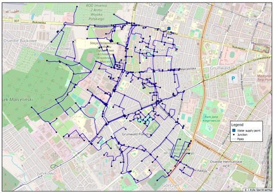
Figure 9. Analysed water supply system.

The changes in water demand during the day (pattern) were assumed as typical for settlements with residential functions. It was assumed that the required pressure in all nodes was 20 mH₂O (2 bar) and the water loss was 15%. The analyses were conducted for 1 d, with 1-h time steps (24 time steps in total).

The results of the calculation can be presented on maps, which show the location of places where the exergy destructions occur (Attachment 1). Figure S1 (Attachment 1) presents units of exergy destructions (W/m³) in pipes, Figures S2 and S3 (Attachment 1) present visualisation of exergy destruction for nodes. For the complex evaluation of the overall system, exergy balance was developed based on Equation (32):

$${\displaystyle \sum }{\mathrm{B}}_{\mathrm{r},\mathrm{out}}={\displaystyle \sum }{\mathrm{B}}_{\mathrm{use}}+{\displaystyle \sum }{\mathsf{\delta }\mathrm{B}}_{\mathrm{exc}}+{\displaystyle \sum }{\mathsf{\delta }\mathrm{B}}_{\mathrm{loss}}+{\displaystyle \sum }{\mathsf{\delta }\mathrm{B}}_{\mathrm{p}}$$

(32)

where:

• ${\displaystyle \sum }{\mathrm{B}}_{r,\mathrm{use}}$—the sum of exergy outflow from reservoir [kWh],
• ${\displaystyle \sum }{\mathrm{B}}_{\mathrm{use}}$—the sum of usable exergy outflow from the thermodynamical system [kWh],
• ${\displaystyle \sum }{\mathsf{\delta }\mathrm{B}}_{\mathrm{exc}}$—the sumof internal exergy destructions caused by excess pressure higher than required in the node [kWh],
• ${\displaystyle \sum }{\mathsf{\delta }\mathrm{B}}_{\mathrm{loss}}$—the sum of exergy destructions, caused by loss of water mass because of leakage [kWh]
• ${\displaystyle \sum }{\mathsf{\delta }\mathrm{B}}_{\mathrm{p}}$—the sum of internal exergy destruction in the pipes (caused by friction) [kWh].

In the analysed case, ${\displaystyle \sum }{\mathrm{B}}_{\mathrm{out},\mathrm{res}}= 6534 [\mathrm{kWh}]$, ${\displaystyle \sum }{\mathrm{B}}_{\mathrm{use}}=991 [\mathrm{kWh}]$, ${\displaystyle \sum }{\mathsf{\delta }\mathrm{B}}_{\mathrm{exc}}=3939 [\mathrm{kWh}]$, ${\displaystyle \sum }{\mathsf{\delta }\mathrm{B}}_{\mathrm{loss}}=870 [\mathrm{kWh}]$, and ${\displaystyle \sum }{\mathsf{\delta }\mathrm{B}}_{\mathrm{p}}=732 [\mathrm{kWh}]$. The graphical representation of the exergy balance is shown in Figure 10.

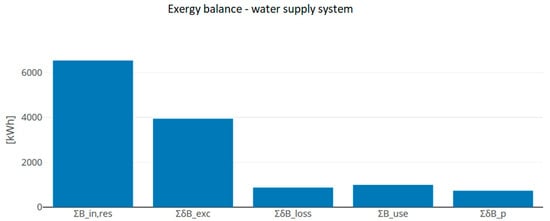
Figure 10. Exergy balance chart for analysed water-supply system.

As analysed, the largest exergy destruction resulted from maintaining higher than the required pressure in the water-supply network. Exergy destruction in pipes has also significant impact on the exergy balance. Figure 11 shows the distribution of exergy losses caused by keeping the pressure in nodes higher than required. Figure 12 presents the distribution of exergy loss in pipes (due the friction).

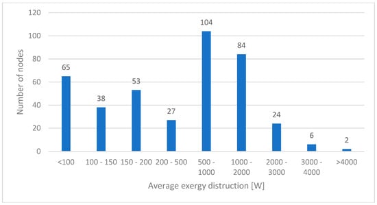
Figure 11. Distribution of exergy destruction in nodes.

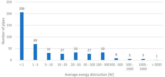
Figure 12. Distribution of exergy destruction in pipes.

4.2. Water Treatment Plant

In the second case, the exergy balance for a water treatment plant was conducted, consisting of a water intake area, treatment station, and pumping station. Water intake consisted of two wells. Water from the wells was transported by pipe systems to a water treatment station, where it was aerated (in a closed aerator), and then pumped through filters to the clean water tank. From the clean water tank, it was pumped to the water distribution system by a second stage pumping station. Figure 13 shows a diagram of the analysed water treatment plant.

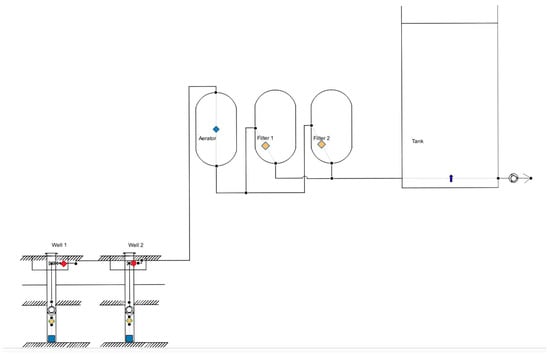
Figure 13. Analysed water treatment plant.

The results of the calculations were the exergy models for each element of the water treatment station. Figure S4 (attachment 1) presents units of exergy destructions (W/m³) in the water treatment plant. For the complex evaluation of the overall system, exergy balance was developed based on Equation (33):

$$\begin{gathered} {\displaystyle \sum }{\mathrm{B}}_{\mathrm{in},\mathrm{pump}}+{\displaystyle \sum }{\mathrm{B}}_{\mathrm{r},\mathrm{out}}+{\displaystyle \sum }{\mathrm{B}}_{\mathrm{use}}= \\ ={\displaystyle \sum }{\mathsf{\delta }\mathrm{B}}_{\mathrm{p}}+{\displaystyle \sum }{\mathsf{\delta }\mathrm{B}}_{\mathrm{pump}}+{\displaystyle \sum }{\mathsf{\delta }\mathrm{B}}_{\mathrm{fill}}+{\displaystyle \sum }{ \mathsf{\delta }\mathrm{B}}_{\mathrm{aer}}+{\displaystyle \sum }{\mathsf{\delta }\mathrm{B}}_{\mathrm{v}}+{\displaystyle \sum }{\mathsf{\delta }\mathrm{B}}_{\mathrm{well}}+{\displaystyle \sum }{\mathrm{B}}_{\mathrm{t}}+{\displaystyle \sum }{\mathsf{\delta }\mathrm{B}}_{\mathrm{loss}}+{\displaystyle \sum }{\mathsf{\delta }\mathrm{B}}_{\mathrm{exc}} \end{gathered}$$

(33)

where:

• ${\displaystyle \sum }{\mathrm{B}}_{\mathrm{in},\mathrm{pump}}$—the sum of exergy inflow to the thermodynamical system (inlet pipse) [kWh]
• ${\displaystyle \sum }{\mathrm{B}}_{\mathrm{r},\mathrm{out}}$—the sum of exergy outflow from reservoir [kWh], ${\displaystyle \sum }{\mathrm{B}}_{\mathrm{use}}$—the sum of usable exergy outflow from the thermodynamical system [kWh],
• ${\displaystyle \sum }{\mathrm{B}}_{\mathrm{use}}$—the sum of usable exergy outflow from the thermodynamical system [kWh],
• ${\displaystyle \sum }{\mathsf{\delta }\mathrm{B}}_{\mathrm{p}}$—the sum of internal exergy destruction in the pipes (caused by friction) [kWh],
• ${\displaystyle \sum }{\mathsf{\delta }\mathrm{B}}_{\mathrm{pump}}$—the sum of internal exergy destruction in the pump [kWh].
• ${\displaystyle \sum }{\mathsf{\delta }\mathrm{B}}_{\mathrm{fill}}$—the sum of internal exergy destruction in the filter [kWh].
• ${\displaystyle \sum }{ \mathsf{\delta }\mathrm{B}}_{\mathrm{aer}}$—the sum of internal exergy destruction in the aerator [kWh].
• ${\displaystyle \sum }{\mathsf{\delta }\mathrm{B}}_{\mathrm{v}}$—the sum of internal exergy destruction in the valves (minor losses) [kWh].
• ${\displaystyle \sum }{\mathsf{\delta }\mathrm{B}}_{\mathrm{well}}$—the sum of internal exergy destruction in well [kWh].
• ${\displaystyle \sum }{\mathrm{B}}_{\mathrm{t}}$—exergy stored in tank at the end simulation [kWh],
• ${\displaystyle \sum }{\mathsf{\delta }\mathrm{B}}_{\mathrm{loss}}$—the sum of exergy destructions, caused by loss of water mass because of leakage [kWh]

In the analysed case, ${\displaystyle \sum }{\mathrm{B}}_{\mathrm{in},\mathrm{pump}}=1277 [\mathrm{kWh}]$, ${\displaystyle \sum }{\mathrm{B}}_{\mathrm{r},\mathrm{in}}= 697 [\mathrm{kWh}]$, ${\displaystyle \sum }{\mathrm{B}}_{\mathrm{use}}= 110 [\mathrm{kWh}]$, ${\displaystyle \sum }{\mathsf{\delta }\mathrm{B}}_{\mathrm{p}}= 25 [\mathrm{kWh}]$, ${\displaystyle \sum }{\mathsf{\delta }\mathrm{B}}_{\mathrm{pump}}=533 [\mathrm{kWh}]$,${\displaystyle \sum }{\mathsf{\delta }\mathrm{B}}_{\mathrm{fill} }=30 [\mathrm{kWh}]$, ${\displaystyle \sum }{\mathsf{\delta }\mathrm{B}}_{\mathrm{aer}}= 5 [\mathrm{kWh}]$, ${\displaystyle \sum }{\mathsf{\delta }\mathrm{B}}_{\mathrm{v}}=8 [\mathrm{kWh}]$, ${\displaystyle \sum }{\mathsf{\delta }\mathrm{B}}_{\mathrm{well}}=600 [\mathrm{kWh}]$, ${\displaystyle \sum }{\mathrm{B}}_{\mathrm{t}}=119 [\mathrm{kWh}]$, ${\displaystyle \sum }{\mathsf{\delta }\mathrm{B}}_{\mathrm{loss}}=0$, and ${\displaystyle \sum }{\mathsf{\delta }\mathrm{B}}_{\mathrm{exc}}=1083 [\mathrm{kWh}]$. The graphic representation of the exergy balance is presented in Figure 14.

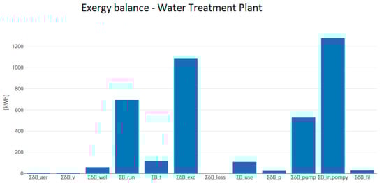
Figure 14. Exergy balance for the water treatment plant.

The analysis shows that the biggest exergy destruction resulted from maintaining a higher than required pressure at the station outlet. Figure 15 presents the rate of exergy destruction during simulation time.

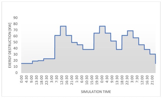
Figure 15. The rate of exergy destruction during simulation time.

5. Discussion

In this study, the exergy models for each part of a system were developed, which allowed the calculation of exergy models and results presentation on maps (Attachment 1). Using the developed tools, the exergy destruction calculations were conducted for sample elements of a water-supply system. Unit indicators of exergy destructions and exergy balance were developed, which could be used to evaluate the system. The visualisation allowed the detection of weak points in the system and the exploration of opportunities to increase the efficiency of energy transformation.

Exergy models are particularly important for mapping opportunities to increase the energy efficiency of the entire system. Graphical analysis (Attachment 1) makes it possible to check which elements have the highest exergy destructions. In the first case (water-supply system) the highest exergy destructions were caused by keeping the pressure in the node higher than required. Detailed analysis shown that a small number of node and pipes are responsible for a significant part of the exergy destruction (Figure 11 and Figure 12). The developed tool made it possible to easily select these nodes and pipes. In the first case study energy efficiency can be increased in two ways: by minimising pressure in the pumping station or by increasing the recovery of energy in the system (in the turbines). Energy recovery from the water-supply system is possible primarily through the use of turbines with pressure recovery in places where the pressure in the network is higher than required. The maps allow determination of locations where the highest exergy destructions occur, which is correspondingly the place in which the greatest potential gains from modernisation can be obtained.

In the second case, the highest exergy destruction results from destructions in pump motors and from excess pressure in the pumping station. It is necessary to analyse the results if the pump is changed to a more effective one. The analysis of the graph (Figure 15) showed that the pressure is maintained higher than required throughout the simulation period. To improve the energy efficiency of this system, the control algorithms of the pump should be change. The pressure should be reduce when it is higher than required (eg. by installing a frequency converter). Data analysis (Figure 14) showed that exergy losses in filters and wells are small and do not have a large impact on the total exergy balance. The most important criteria in modernization of these elements should be primarily technological (maintaining adequate water quality). Exergy destruction in this analized case is not an important criterion for wells and filters.

6. Conclusions

This study presents exergy models for a water-supply system, which are based on the first and second law of thermodynamics. The research shows that:

• Exergy analysis is an effective method of assessing the water supply system. It enables both quantitative and qualitative assessment of energy transformations,
• Analyse of exergy balance allow the determination of the most exergy-consuming elements in the system and assess the possibility of reducing exergy destruction during modernisation,
• The developed tools can be used to support decision making in the design, operation, and maintenance of water-supply systems,
• Using developed open source tool, it is possible to automatically perform an exergy analysis of the system. This approach can be helpful in maintenance processes to determine system insufficiencies.

Future work will be directed toward the development of exergy models for chemical and thermal energy changes in water-supply systems. The development of chemical exergy transformation models will allow for a better understanding of water treatment processes and water-quality changes in supply networks. A model of thermal exergy transformation can be useful to assess the potential of the water-supply system as the lower heat source for heat pumps. The exergy assessment is one of the important aspects of the overall assessment of the water-supply system. As discussed, it allows the identification of the weakest points in the system. Final investment decisions must take into account the financial aspect of the organisation as well as the safety and reliability of the system operation. In future works, we plan to develop the proposed methodology with a multi-criteria and exergo-economic analysis.

References

- Bylka, J.; Mroz, T. A Review of Energy Assessment Methodology for Water Supply Systems. Energies 2019, 12, 4599. [Google Scholar] [CrossRef]
- Cabrera, E.; Pardo, M.A.; Cobacho, R. Energy Audit of Water Networks. J. Water Resour. Plan. Manag. 2010, 136, 669–677. [Google Scholar] [CrossRef]
- Mamade, A.; Loureiro, D.; Alegre, H.; Covas, D. A comprehensive and well tested energy balance for water supply systems. Urban Water J. 2017, 14, 853–861. [Google Scholar] [CrossRef]
- Walski, T. Energy Balance for a Water Distribution System. In Proceedings of the World Environmental and Water Resources Congress 2016, West Palm Beach, FL, USA, 22–26 May 2016. [Google Scholar]
- Dziedzic, R.; Karney, B.W. Energy Metrics for Water Distribution System Assessment: Case Study of the Toronto Network. J. Water Resour. Plan. Manag. 2015, 141, 04015032. [Google Scholar] [CrossRef]
- Hashemia, S.; Filion, Y.R.; Speight, V.L. Pipe-level Energy Metrics for Energy Assessment in Water Distribution Networks. In Proceedings of the Procedia Engineering (119), 3th Computer Control for Water Industry Conference, CCWI 2015, Leicester, UK, 2–4 September 2015. [Google Scholar]
- Szargut, J.; Petela, R. Egzergia; WNT: Warszawa, Poland, 1965. [Google Scholar]
- Dincer, I.; Rosen, M.A. Exergy; Elsevier Ltd.: Amsterdam, The Netherlands, 2013. [Google Scholar]
- Shukuya, M. Bio-Climatology for Built Environment; CRC Press: Boca Raton, FL, USA, 2019. [Google Scholar]
- Shukuya, M. Exergy Theory and Applications in the Built Environment; Springer Verlag: London, UK, 2013. [Google Scholar]
- Szargut, J. International progress in second law analysis. Energy 1980, 5, 709–718. [Google Scholar] [CrossRef]
- Boroumand Jazi, G.; Rismanchi, B.; Rahman, S. A review on exergy analysis of industrial sector. Renew. Sustain. Energy Rev. 2013, 27, 198–203. [Google Scholar] [CrossRef]
- Rijs, A.; Mróz, T. Exergy evaluation of a heat supply system with vapor compression heat pumps. Energies 2019, 12, 1028. [Google Scholar] [CrossRef]
- Çomaklı, K.; Yüksel, B.; Çomaklı, Ö. Evaluation of energy and exergy losses in district heating network. Appl. Therm. Eng. 2004, 24, 1009–1017. [Google Scholar] [CrossRef]
- Reddy, V.S.; Kaushik, S.C.; Tyagi, S.K.; Panwar, N. An Approach to Analyse Energy and Exergy Analysis of Thermal Power Plants: A Review. Smart Grid Renew. Energy 2010, 1, 143–152. [Google Scholar] [CrossRef]
- Shukuya, M. Exergetic review on passive and active systems for ventilation. In Proceedings of the IOP Conference Series Materials Science and Engineering; IOP Science: Bristol, UK, 2019. [Google Scholar]
- Verkhivker, G.P.; Kosoy, B.V. On the exergy analysis of power plants. Energy Conversat. Manag. 2001, 42, 2053–2059. [Google Scholar] [CrossRef]
- Aljundi, I.H. Second-law analysis of a reverse osmosis plant in Jordan. Desalination 2009, 239, 207–215. [Google Scholar] [CrossRef]
- Blanco-Marigorta, A.M.; Masi, M.; Manfrida, G. Exergo-environmental analysis of a reverse osmosis desalination plant in Gran Canaria. Energy 2014, 76, 223–232. [Google Scholar] [CrossRef]
- Sharqawy, M.H.; Zubair, S.M.; Lienhard, J.H. Second law analysis of reverse os-mosis desalination plants: An alternative design using pressure retarded osmo-sis. Energy 2011, 36, 6617–6626. [Google Scholar] [CrossRef]
- Wall, G.; Gong, M. On Exergetics, Economics and Desalination; Sweden Exergy Consultant: Mölndal, Sweden, 1997. [Google Scholar]
- Martínez, A.; Uche, J.; Rubio, C.; Carrasquer, B. Exergy cost of water supply and water treatment technologies. Desalination Water Treat. 2010, 24, 123–131. [Google Scholar] [CrossRef]
- Fitzsimons, L. A Detailed Study of Desalination Exergy Models and Their Application to a Semi-Conductor Ultra-Pure Water Plant. Ph.D. Thesis, Dublin City University, School of Mechanical and Manufacturing Engineering, Dublin, Ireland, 2011. [Google Scholar]
- Chen, G.Q.; Ji, X. Chemical exergy based evaluation of water quality. Ecol. Model. 2007, 200, 259–268. [Google Scholar] [CrossRef]
- Bylka, J.; Mróz, T. The exergy evaluation of municipal water supply systems. In Zaopatrzenie w Wodę, Jakość i Ochrona Wód-WODA 2016; Dymaczewski, Z., Jeż-Walkowiak, J., Urbaniak, A., Eds.; PziTS: Poznan, Poland, 2016; pp. 43–57. [Google Scholar]
- Tai, S.; Matsushige, K.; Goda, T. Chemical exergy of organic matter in wastewater. Int. J. Environ. Stud. 1986, 27, 301–315. [Google Scholar] [CrossRef]
- Mora, C.H. Environmental exergy analysis of wastewater treatment plants. Therm. Eng. 2006, 5, 24–29. [Google Scholar] [CrossRef]
- Hellström, D. An Exergy Analysis for a Wastewater Treatment Plant: An Estimation of the Consumption of Physical Resources. Water Environ. Res. 1997, 69, 44–51. [Google Scholar] [CrossRef]
- Hellström, D. Exergy analysis of nutrient recovery processes. Water Sci. Technol. 2003, 48, 27–36. [Google Scholar] [CrossRef]
- Fitzsimons, L. Assessing the thermodynamic performance of Irish municipal wastewater treatment plants using exergy analysis: A potential benchmarking approach. J. Clean Prod. 2016, 131, 387–398. [Google Scholar] [CrossRef]
- Martínez-Gracia, A.; Valero, A.; Uche, J. The hidden value of water flows: The chemical exergy of rivers. Int. J. Thermodyn. 2012, 15, 17. [Google Scholar] [CrossRef][Green Version]
- Rossman, L. Epanet 2 User Manual; National Risk Management Research Laboratory; US EPA: Cincinnati, OH, USA, 2000.
- Shukuya, M. Flow and Circulation of Matter. In Bio-Climatology for Built Environment; CRC Press: Boca Raton, FL, USA, 2019. [Google Scholar]
- Sitzenfrei, R.; Fach, S.; Kleidorfer, M.; Urich, C.; Rauch, W. Dynamic virtual infrastructure benchmarking: DynaVIBe. Water Sci. Technol. Water Supply 2010, 10, 600–609. [Google Scholar] [CrossRef]
- Sitzenfrei, R.; Möderl, M.; Hellbach, C.; Rauch, W. Application of a Stochastic Test Case Generation for Water Distribution Systems. In Proceedings of the World Environmental and Water Resources Congress 2011: Bearing Knowledge for Sustainability; Beighley, R.E., Killgore, M.W., Eds.; American Society of Civil Engineers: Restom, WV, USA, 2011. [Google Scholar]
- Sitzenfrei, R.; Möderl, M.; Rauch, W. Automatic generation of water distribution systems based on GIS data. Environ. Model. Softw. 2013, 47, 138–147. [Google Scholar] [CrossRef] [PubMed]
Publisher’s Note: MDPI stays neutral with regard to jurisdictional claims in published maps and institutional affiliations. |
© 2020 by the authors. Licensee MDPI, Basel, Switzerland. This article is an open access article distributed under the terms and conditions of the Creative Commons Attribution (CC BY) license (http://creativecommons.org/licenses/by/4.0/).