Modeling of Limestone Dissolution for Flue Gas Desulfurization with Novel Implications

Abstract

Solid-liquid dissolution is a central step in many industrial applications such as pharmaceutical, process engineering, and pollution control. Accurate mathematical models are proposed to improve reactor design and process operations. Analytical methods are significantly beneficial in the case of iterative methods used within experimental investigations. In the present study, a detailed analytical solution for the general case of solid particles dissolving in multiphase chemical reaction systems is presented. In this model, the authors consider a formulation that considers the particles’ shape factor. The general case presented could be utilized within different problems of multiphase flows. These methods could be extended to different cases within the chemical engineering area. Examples are illustrated here in relation to limestone dissolution taking place within the Wet Flue Gas Desulfurization process, where calcium carbonate is dissolving in an acidic environment. The method is the most common used technology to abate SO₂ released by fuel combustion. Limestone dissolution plays a major role in the process. Nevertheless, there is a need for improvements in the optimization of the WFGD process for scale-up purposes. The mathematical model has been tested by comparison with experimental data from several mild acidic dissolution assays of sedimentary and metamorphic limestone. We have found that R² ⊂ 0.92 ± 0.06 from dozens of experiments. This fact verifies the model qualifications in capturing the main drivers of the system.

1. Introduction

Solid liquid dissolution is a central step in many processes: pharmaceutical, process engineering, pollution control, and many others. The basic modeling of solid dissolution goes back to the Noyes-Whitney-Nernst and Levich models [1,2]. However, it is quite common that these models, or variations of them, are still used in the modern literature [3]. The shape and motion of the particles affect the solid dissolution process, and this factor complicates the modeling involved. Many models have been applied in the literature to match experimental data with theory; some attempts date back more than 50 years [4,5]. In addition, the modeling of solid particles’ dissolution can be found in the most recent scientific texts [3,6].

Applications of these models could be implemented in the field of chemical reaction engineering in the process industry; for instance, to solve problems of particles’ mixing, or they can be applied to give important information in relation to health implementation [7]. One clear example is the case of external supplements and curative aids distributed in the form of tablets to be dissolved within our bodies at acidic conditions.

The solid dissolution could also consider different environments and boundaries, such as in the case of diversely shaped channels [8]. Mathematical modeling, together with experimental results regarding the fluid dynamics involved, will contribute to establishing appropriate rules for design, scale up, and operation control [9].

In case the mass balance is well described by ordinary differential equations and there are parameters describing, for instance, the mass transfer coefficient and the diffusivity of the dissolving element, those parameters could be evaluated by implementing a software procedure to obtain a suitable regression coefficient, and their value could be obtained by an iterative method. One example is the Levenberg-Marquardt method [10]. However, if experimental data are available on the dissolved concentrations vs. time and diverse models are tested to find the correct value of the transport parameters, there will be a major difference in computational time if numerical methods are implemented. In practice, analytical solutions significantly speed up this process [11].

Referring to environmental processes and pollution reduction, it is well known that there is always a pressing need to reduce energy consumption and the amount of pollutants into the atmosphere. The world population accounts for more than seven billion people, and it is forecasted to increase to more than nine billion by 2040 [12,13]. Therefore, the total energy demand is also increasing at a reasonable speed. As a matter of fact, the world energy consumption will be around $8.44\times {10}^{14 }$ MJ/year by 2040 [14]. These numbers suggest that it could be difficult soon to avoid pollution and utilize only renewable energy resources. Coal and oil are utilized extensively in the world, and for this reason, any improvement to the coal-fired power plants technology would represent a large step toward pollution prevention.

There is reason to believe that coal will be utilized for some decades ahead, and the reserves of this sources are still large in the world [15]. Coal contains large quantities of sulfur [16], and it is well known that when combusted, large quantities of SO₂ are released by the process. For instance, some super-high sulfur contents can be found in particular samples from China [10]. SO₂ and any forms of SO_x should be removed carefully from the produced flue gas, since SO₂ can react with the atmospheric moisture and produce sulfuric acid, which is precipitated then under the form of acid rains. This damages all living species [17].

Wet Flue Gas Desulfurization (WFGD) is the most used technology utilized to precipitate SO₂ in the form of gypsum [18] (

Table 1. Main steps and reactions in Wet Flue Gas Desulfurization (WFGD) [11].

Rate Determining Steps	Reactions
Absorption of gaseous SO2 in liquid water	${\mathrm{SO}}_2+{\mathrm{H}}_2\mathrm{O}\rightleftarrows {\mathrm{H}}^{+}+{\mathrm{HSO}}_3^{-}$ ${\mathrm{HSO}}_3^{-}\rightleftarrows {\mathrm{H}}^{+}+{\mathrm{SO}}_3^{2-}$
Oxidation of ${\mathrm{HSO}}_3^{-}$ (liquid phase)	${\mathrm{HSO}}_3^{-}+\frac{1}{2}{\mathrm{O}}_2\rightleftarrows {\mathrm{H}}^{+}+{\mathrm{SO}}_4^{2-}$
Solid limestone is dissolving in acidic environment (pH 5.5, industrial process)	${\mathrm{HSO}}_4^{2-}\rightleftarrows {\mathrm{SO}}_4^{2-}+{\mathrm{H}}^{+}$ ${\mathrm{CaCO}}_3\rightleftarrows {\mathrm{Ca}}^{2+}+{\mathrm{CO}}_3^{2-}$ ${\mathrm{CO}}_2+{\mathrm{H}}_2\mathrm{O}\rightleftarrows {\mathrm{HCO}}_3^{-}+{\mathrm{H}}^{+}$ ${\mathrm{HCO}}_3^{-}\rightleftarrows {\mathrm{CO}}_3^{2-}+{\mathrm{H}}^{+}$ ${\mathrm{H}}_2\mathrm{O}\rightleftarrows {\mathrm{H}}^{+}+{\mathrm{OH}}^{-}$
Crystallization of gypsum	${\mathrm{Ca}}^{2+}+{\mathrm{SO}}_4^{2-}+2{\mathrm{H}}_2\mathrm{O}\rightleftarrows {\mathrm{CaSO}}_4·2{\mathrm{H}}_2\mathrm{O}$

). This technology is not new, and very little changes have been implemented for this process in recent years.

Nevertheless, this does not mean that there is no margin for improvements. Since the system accounts for almost 3% of the entire energy produced by the power plant [19], mathematical modeling and optimization of the process could give reasonable impact on the energy consumption and therefore pollution reduction. Furthermore, improvement of the method used is also possible with novel techniques and the usage of ultrasonic power [20].

Limestone dissolution represents the key step process in WFGD, since this would represent the limiting two-phase step development among the ones shown in Table 1. An accurate mathematical modeling of the limestone dissolution process would lead to better reactor design and operation management in WFGD. This will result in energy saving and economic impact.

The main goal of the work is to show a simpler procedure to predict the acidic dissolution of limestone particles for flue gas desulfurization purposes. The modeling of limestone dissolution has been carried out by our research team considering several samples that originated in diverse regions of the world. Nevertheless, limestone dissolution kinetics is also to be considered important in relation to other aspects, which are not necessarily are related to industrial processes. For example, this phenomenon is to be taken into account considering the vast presence of carbonate rocks within the oceans and in relation to climate change [14].

In the present work, a detailed analytical method is given for a mass balance describing solid dissolution in acidic environments. The assumption is that the component of interest is dissolving in a perfectly mixed batch system. Here, we investigated the possibility of considering the particle’s shape factor, and the purpose is to give a general method that could be adopted in case of diverse particle forms. This was done by reporting a detailed analytical solution that has never been presented in the literature and can be extended to different processes. In the present study, the limestone dissolution operated within the Wet Flue Gas Desulfurization (WFGD) process conditions is contrasted successfully against experimental dissolution assays. For this technology, there is a margin of improvements by developing novel technology and by optimizing process conditions [19,20,21].

Despite the simplicity of the approach, one can still get some information on the underlying dynamics, which can be used in lumped models to describe a global reactor behavior or contributing to provide a reliable theory that can predict changes in an already installed reactor performance with changes in operating parameters, such as feed conditions, since it is possible to use it under the industrial environment without the need for complex time-consuming simulations. In addition, we are providing a statistical methodology to verify the model, which is a robust tool to predict the reactivity of the limestone particles.

2. Materials and Methods

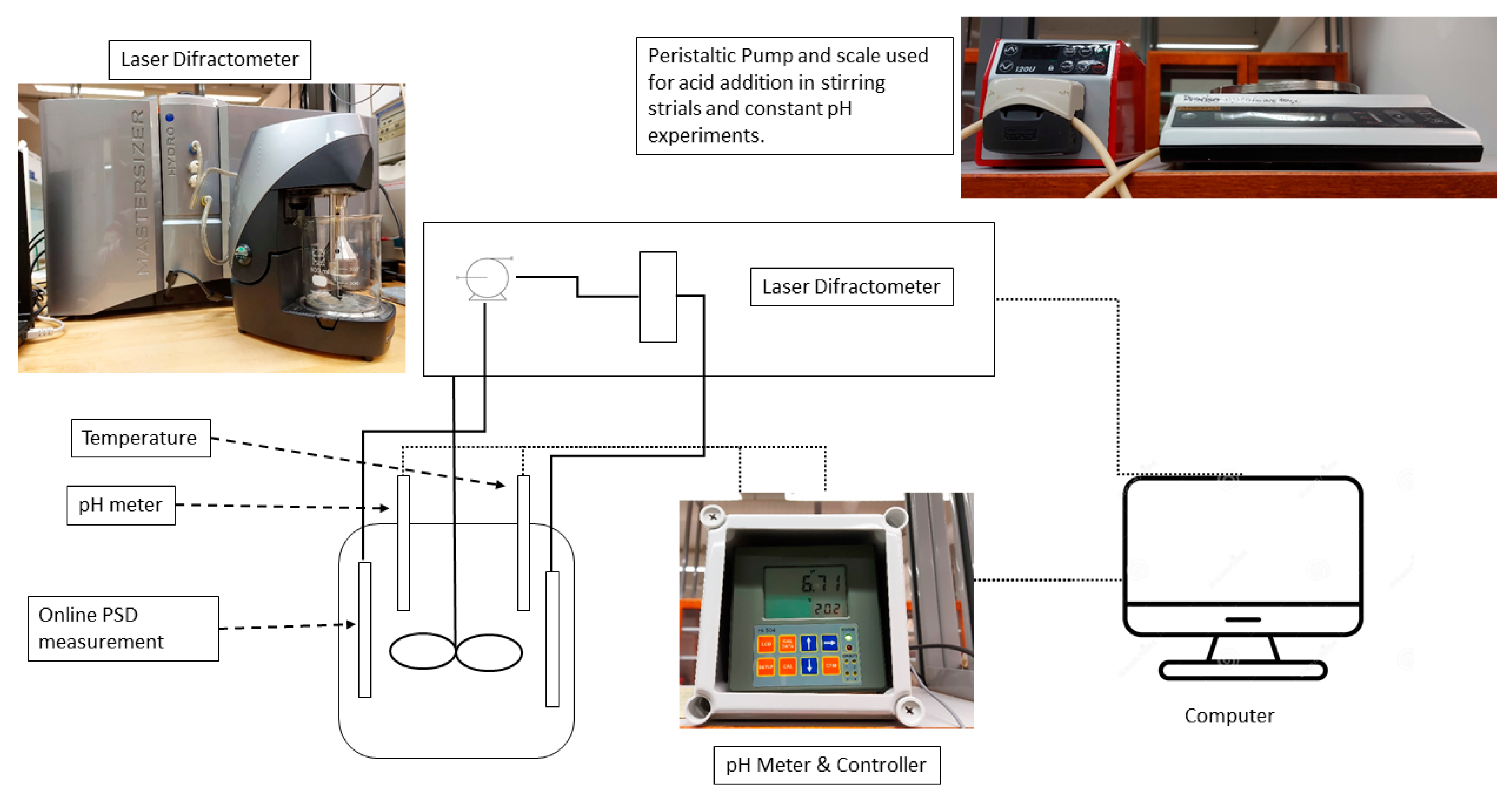
2.1. Experimental Procedure

The limestone dissolution was investigated by providing an analytical description, which is based on a mass balance described in Section 2.2 and compared with results of an acidic environment and transient conditions. Two kinds of limestone samples were used; one was classified as Metamorphic Limestone and one was classified as Sedimentary Limestone. The first one has been formed in the Proterozoic age (1900 Ma), while the Sedimentary Limestone has formed within the Jurassic age (150 Ma). The samples were arranged to the required measure by crushing (jaw crusher) and then sieving. The sieve used for the measures proposed here has a range of 212–250 $\mathsf{\mu }$m. The density of the samples was evaluated by a helium pycnometer (AccuPyc 1330).

Scanning Electron Microscope (SEM) images were recorded with a Leo Gemini 1530 (Leo, Oberkochen, Germany) equipped with a secondary electron, a backscattered electron, and In-Lens detectors. Since calcite is an electrical insulator, all the samples were treated with carbon deposition to ensure the conductivity of the surface. The micrographs were obtained using secondary electrons.

The composition of the samples is given by X-Ray Fluorescence (XRF). Vitrification of the sample powders for XRF measurements was done by melting the sample and lithium tetraborate in an oven at 1040 °C in a platinum crucible. The sample to lithium tetraborate ratio was 1 to 5. The XRF measurements were done with a PW2400 (PANalytical, Almelo, the Netherlands), which is a wavelength dispersive XRF (WDXRF). An Rh tube was operated at 50 kV and 60 mA (40 and 50 mA in the case of Fe and Mg, respectively) focused over the sample to create X-rays by the Auger effect. Characteristic wavelengths of the elements were dispersed from the emission spectrum by crystals. Elements present in the samples and their concentrations were identified according to their emitted wavelengths and intensities using a gas flow detector containing a mixture of argon and methane.

For this investigation, the dissolution of limestone samples was performed into a beaker containing 0.5 L of deionized water. The particle size distribution (PSD) was measured by laser diffractometry (Malvern Mastersizer 3000, Malvern Hydro EV system). The laser diffractometer has a single unit for particle measurements of wet dispersions. The unit is equipped with a built-in stirrer that has 3 blades pointed downwards. The propeller has a diameter of 0.03 m. The right amount of the mass sample was chosen to give statistically relevant measurements by checking if the obscuration bar of the software was in the range between 2% and 24%. The obscuration is a parameter related to the laser, and it helps to determine the mass of the sample when it is added to the dispersant. It can be defined as the amount of laser light lost as a result of the addition of the sample into the analyzer beam. For this reason, the solid content of the dispersion ranged between 1.5 and 6 g/L. The sample amount was measured on a Precisa Gravimetrics 410 AM-FR scale.

To assure that all the particles were resuspended into the slurry, a velocity of 2300 rpm was used for all the experiments. This was estimated by calculations proposed in literature [22] and by verifying it experimentally. As a matter of fact, we have done experimental trials maintaining the pH value constant and measuring the acid consumption at different stirring velocities. When no difference in acid consumption was recorded regardless of the increase in stirring speed, that pointed out the sufficiency in stirring speed.

pH measurements were taken by a pH electrode (double junction with a built-in reference and epoxy body VWR electrode), and the temperature was recorded by a Pt-100 temperature sensor. The pH meter was calibrated before each measurement using pH buffers of 4.01 and 7.01 at room temperature. The equipment also consists of a pH controller (Hanna Instruments, Kungsbacka, Sweden) in case a constant pH is desired, as in the case of the stirring speed trials. A scheme of the experimental set-up used for the dissolution tests is presented in Figure 1.

The experiments done in this work were executed in accordance to a free drift method [23], which has been modified to a stepwise titration method [24]. The difference between the two methods is simply related to the amount of acid added to the solution at each step.

All the experiments were performed adding hydrochloric acid (1 mL of HCl, 1 mol/L) into the limestone-water slurry, and the reaction could proceed until the pH is nearly constant. The values of pH and temperature were recorded by means of the software HI92500 (Hanna Instruments, Kungsbacka, Sweden), which allowed recordings every 5 s.

2.2. Mathematical Modeling

The following is a detailed analytical derivation for a general case where the mass balance for the dissolution of a solid in presence of a reactive species is described by an ordinary differential equation: Equation (3). Regarding this study, the dissolution of limestone in transient acidic conditions is given as an example. For more detail, consider the calcium carbonate dissolution reactions:

$${\mathrm{CaCO}}_{3\left(\mathrm{s}\right)}+{\mathrm{H}}_{\left(\mathrm{aq}\right)}^{+} \leftrightarrow {\mathrm{Ca}}_{\left(\mathrm{aq}\right)}^{2+}+{\mathrm{HCO}}_{3\left(\mathrm{aq}\right)}^{-}$$

(1)

$${\mathrm{HCO}}_{3\left(\mathrm{aq}\right)}^{-}+{\mathrm{H}}_{\left(\mathrm{aq}\right)}^{+} \leftrightarrow {\mathrm{H}}_2{\mathrm{O}}_{\left(\mathrm{l}\right)}+{\mathrm{CO}}_{2\left(\mathrm{aq}\right)}$$

(2)

The rate-determining step is assumed to be reaction (1). In Solid-liquid reactions, the surface area of solid available per volume of liquid, also referred as the reactive surface, is the key factor determining the rate of reaction. The shrinking sphere model [25] can be applied successfully in some cases, although it has been shown that it is not suitable for cases where solids differ from spherical shapes [21]. The reaction order with respect to the solid in the generalized form can be written as $C_s^{\left(1-\frac{1}{d}\right)}$, where Cs is the solid concentration and d is a shape factor. The values of d could have diverse rational forms depending on the shape considered; for spherical particles, it is taken as 3. In practice, Equation (3) presented below is derived by considering the dissolution rate for a dissolving specie $C_s$. This rate is directly proportional to the same concentration of solids into the system, and it is also directly proportional to the concentration of the hydron species $C_{H^{+}}$ within the same system.

This approach is independent of particle morphology and has been applied successfully for different Solid-liquid reactions [26,27]. Thus, the generalized formulation for the solid dissolution can be written according to

$$\frac{d{C}_s}{dt}=-k·C_s^{\left(1-\frac{1}{d}\right)}·C_{H^{+}}$$

(3)

where $C_s$ is denoted as the undissolved element in the form of solid, which is in units of solid mass per total volume. This can be expressed as grams per liter (g/L) percentage of mass to volume (mol/L). Considering Equations (1) and (2) written before, $C_{H^{+}}$ is the molar concentration of hydron ions, k is the reaction rate constant, and d is the so-called shape factor, which is dimensionless and can be calculated according to Aris [4] and simplified as

$$d=\frac{A_p}{V_p}{R}_o,$$

(4)

where $A_p$ is the particle surface area, $V_p$ is the volume, and $R_o$ is the characteristic length of the particle [28]. This equation simply states that the shape factor is a function of the area and volume and depends only upon the shape of the particles independently of their size. In the literature, it is commonly referred that the reaction order has a dependency on the shape factor [29]. In the present study, a straightforward approach is adopted that is based on the mass balance of hydron ion and limestone particles, which are considered the main contributors for the dissolution process. In our modeling, only one additional proportionality constant is considered, and that is the mass transfer coefficient. This is because the system is considered well mixed, and therefore, the diffusivity of hydrogen ions is not a limiting factor for this situation, which will be demonstrated later in Section 3.2 on the basis of the experimental conditions.

One positive aspect of this approach lies in the fact that any shape of a 3-dimensional particle can be implemented in the rate equation as a function of d. For spheres, d is equal to 3, and for infinitely rough, non-spherical particles, d tends to infinity. Performing the substitution $z=\left(1-\frac{1}{d}\right)$, we have:

$$\frac{d{C}_s}{dt}=-k·C_s^z·C_{H^{+}}$$

(5)

By assuming that the dissolution driving force is proportional to the surface area of the particles and the calcium ions in solution, which can be obtained by mass balance from the consumption of hydrogen ions, the following equation is obtained:

$$\frac{d{C}_s}{dt}=-k·A·{\left(C_{H^{+},0}·X\right)}^z·C_{H^{+}};$$

(6)

where $C_{H^{+}}$ is the hydrogen ion concentration and X is the conversion, while the parameter A is the contact area available for the reaction. The dissolution rate is equal to the H⁺ consumption rate; thus, the equation above can be re-written as:

$$\frac{d{C}_{H^{+}}}{dt}=-k·C_{H^{+}}^0{}^z·A·{\left(1-\frac{C_{H^{+}}}{C_{H^{+}}^0}\right)}^z·C_{H^{+}};$$

(7)

where ${(k·C_{H^{+}}^0)}^z$ is defined as the constant k′; therefore,

$$\frac{d{C}_{H^{+}}}{dt}=-k^{\prime }·A·{\left(1-\frac{C_{H^{+}}}{C_{H^{+}}^0}\right)}^z·C_{H^{+}};$$

(8)

with the conditions: $t=0\to C_{H^{+}}=C_{H^{+}}^0$.

The following is a detailed analytical derivation for the solution of this equation. To the author’s knowledge, for calcite acidic dissolution, this has never been presented in the literature. To represent the solution steps in a simpler way, the original equation can be written in the form:

$$\frac{dx}{dt}=-k^{\prime }·A·{\left(1-\frac{x}{c}\right)}^z·x,$$

(9)

where $x=C_{H^{+}}$ and $c=C_{H^{+}}^0$, with the condition $t=0\to x=c$:

The following derivation is valid for any rational number of the form z = a/b. Our available experimental particle size measurements are based on laser diffraction under Fraunhofer theory, so we will consider our particles as spheres; therefore, d = 3 and $z=2/3$. Then, by substitution of $z$, Equation (9) becomes:

$$\frac{dx}{dt}=-k^{\prime }·A{\left(1-\frac{x}{c}\right)}^{2/3}·x$$

(10)

Then, we perform the following variable substitution:$1-\frac{x}{c}=\gamma \stackrel{gives}{\Rightarrow }\frac{c-x}{c}=\gamma \stackrel{gives}{\Rightarrow }dx=-cd\gamma .$ Dividing both terms by $\left(-c\right)$, Equation (10) is now given as:

$$\frac{d\gamma }{dt}=k^{\prime }·A·{\gamma }^{2/3}\left(1-\gamma \right);$$

(11)

this gives

$$\frac{d\gamma }{{\gamma }^{2/3}\left(1-\gamma \right)}=k^{\prime }·A·dt.$$

(12)

Performing the indefinite integral on both terms, we have:

$${\displaystyle \int }{\gamma }^{-\frac{2}{3}}{\left(1-\gamma \right)}^{-1}d\gamma ={\displaystyle \int }{k}^{\prime }·A·dt.$$

(13)

We substitute $\gamma =P^3$, which gives:

$$d\gamma =3P^{2}dP\to {\gamma }^{\frac{2}{3}}=P^2;$$

(14)

and therefore, our integral can be written in the form:

$${\displaystyle \int }\frac{d\gamma }{\sqrt[3]{{\gamma }^2}·\left(1-\gamma \right)}={\displaystyle \int }\frac{3P^2}{P^2\left(1-P^3\right)}dP=3{\displaystyle \int }\frac{1}{\left(1-P^3\right)}dP.$$

(15)

The integral of the right side can be solved if it is put in the convenient form:

$$\frac{1}{\left(1-P^3\right)}=\frac{1}{\left(1-P\right)\left(P^2+P+1\right)}=\frac{a^{\prime }+b^{\prime }·P}{P^2+P+1}+\frac{c^{\prime }}{1-P}$$

(16)

where the goal is now to find the arbitrary constants a′, b′, and c′. The following condition must be fulfilled to comply with Equation (16):

$$c^{\prime }\left(P^2+P+1\right)+\left(1-P\right)\left(a^{\prime }+b^{\prime }P\right)=1$$

(17)

which will give the algebraic system

$$\{\begin{array}{c}{c}^{\prime }+a^{\prime }=1\\ c^{\prime }+b^{\prime }-a^{\prime }=0\\ c^{\prime }-b^{\prime }=0\end{array}.$$

(18)

Therefore, ${\mathrm{c}}^{\prime }=1/3,{\mathrm{b}}^{\prime }=1/3\mathrm{and}{\mathrm{a}}^{\prime }=2/3$. With these results, the term on the right side in Equation (15) is now:

$$3{\displaystyle \int }\frac{1}{\left(1-P^3\right)}dP={\displaystyle \int }\frac{\left(P+2\right)}{P^2+P+1}dP+{\displaystyle \int }\frac{1}{1-P}dP.$$

(19)

The first integral on the right side can be simply written as:

$${\displaystyle \int }\frac{\left(P+2\right)}{P^2+P+1}dP={\displaystyle \int }\frac{\left(2P+1\right)}{2(P^2+P+1)}dP+{\displaystyle \int }\frac{3}{2(P^2+P+1)}dP.$$

(20)

Notice that the first term on the right-hand side presents just the derivative of the denominator in parentheses, while the second term can be written as:

$${\displaystyle \int }\frac{3}{2(P^2+P+1)}dP=\frac{3}{2}{\displaystyle \int }\frac{1}{{\left(P+\frac{1}{2}\right)}^2+\frac{3}{4}}dP=\sqrt{3}ArcTan\left(\frac{2P+1}{\sqrt{3}}\right)+const.$$

(21)

This leads to the two indeterminate forms of the following terms:

$${\displaystyle \int }\frac{\left(P+2\right)}{P^2+P+1}dP=\frac{1}{2}ln\left(P^2+P+1\right)+\sqrt{3}ArcTan\left(\frac{2P+1}{\sqrt{3}}\right)+const,$$

(22)

while the term on the right hand side of Equation (18) is simply:

$${\displaystyle \int }\frac{1}{1-P}dP=-\ln \left(1-P\right)+const.$$

(23)

Then, the final solution for this case would be

$$\frac{1}{2}ln\left(P^2+P+1\right)+\sqrt{3}ArcTan\left(\frac{2P+1}{\sqrt{3}}\right)-\ln \left(1-P\right)+const=k^{\prime }·A·t;$$

(24)

which is translated here with respect to the original variables and parameters $x=C_{H^{+}}$, $c=C_{H^{+}}^0$:

$$\frac{1}{2}ln\left({\left(\sqrt[3]{\left(1-\frac{C_{H^{+}}}{C_{H^{+}}^0}\right)}\right)}^2+\left(\sqrt[3]{\left(1-\frac{C_{H^{+}}}{C_{H^{+}}^0}\right)}\right)+1\right)+\sqrt{3}ArcTan\left(\frac{2\left(\sqrt[3]{\left(1-\frac{C_{H^{+}}}{C_{H^{+}}^0}\right)}\right)+1}{\sqrt{3}}\right)-\ln \left(1-\left(\sqrt[3]{\left(1-\frac{C_{H^{+}}}{C_{H^{+}}^0}\right)}\right)\right)+const=k^{\prime }·A·t$$

(25)

where the integration constant is $-\sqrt{3}ArcTan\left(\frac{1}{\sqrt{3}}\right)=-\frac{\sqrt{3}\pi }{6}=\frac{\pi }{2\sqrt{3}}~0.9069$, which is obtained from the condition $\left(1-\frac{C_{H^{+}}}{C_{H^{+}}^0}\right)=0$ when $t=0$.

3. Results

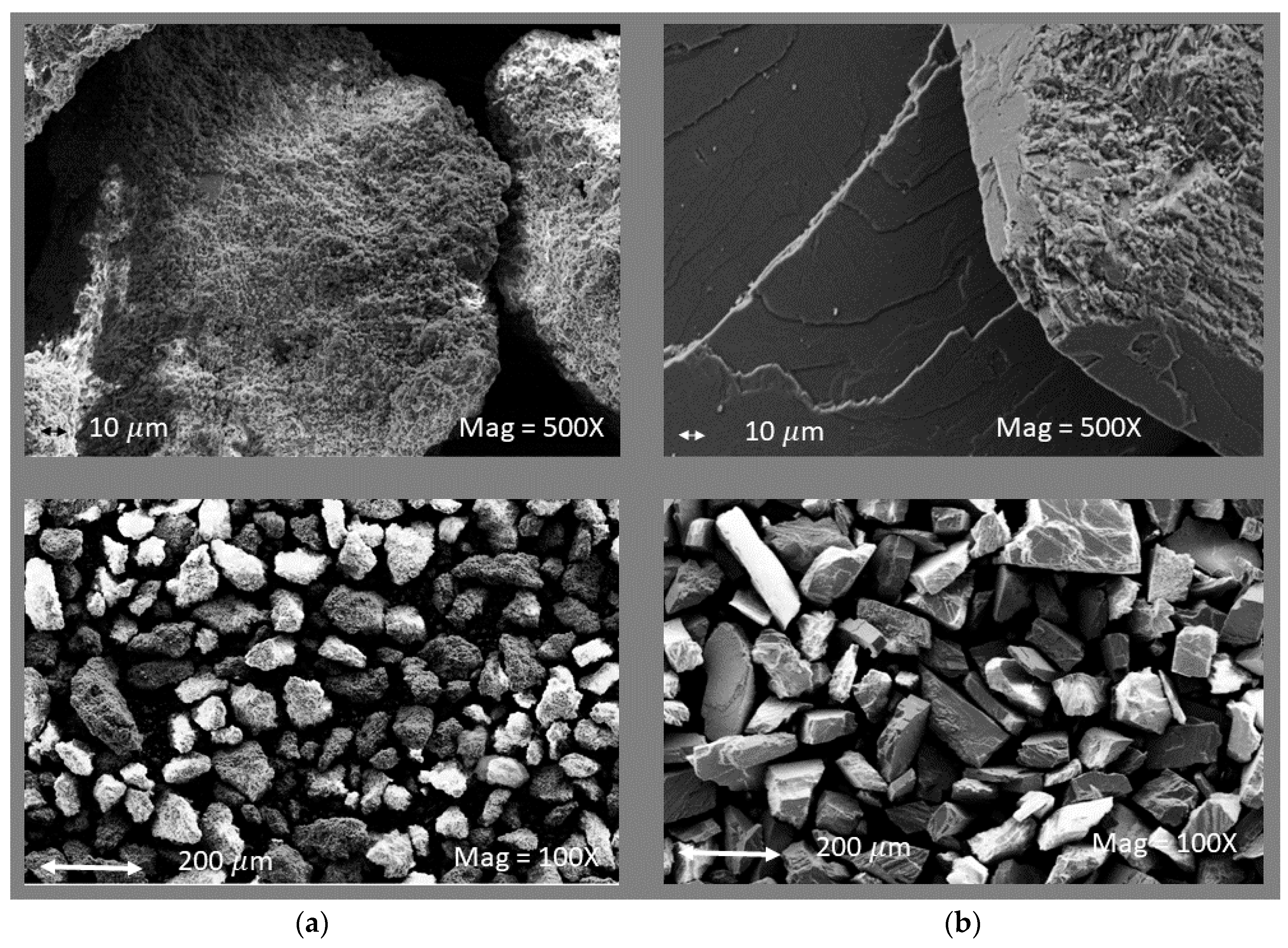
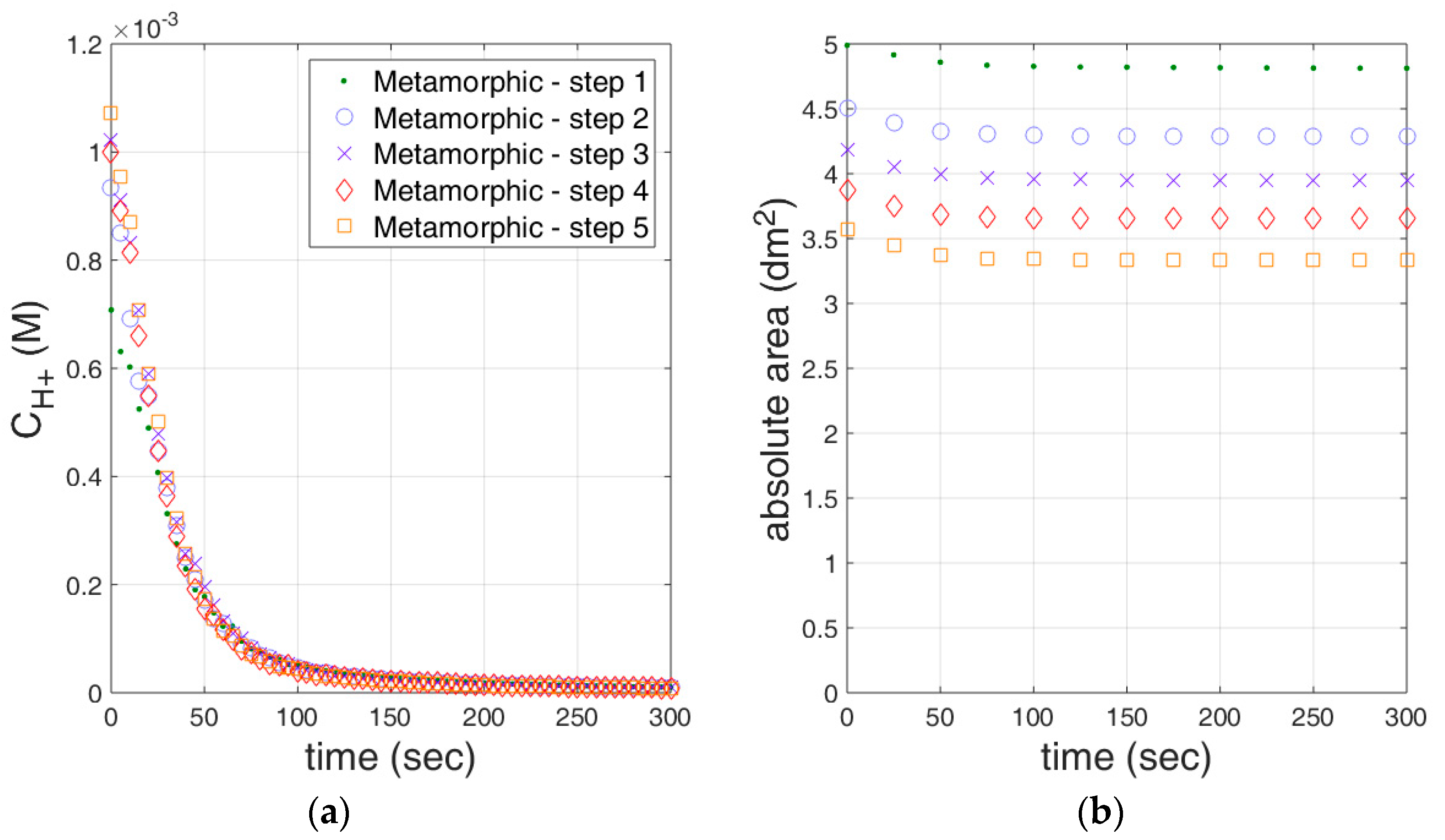
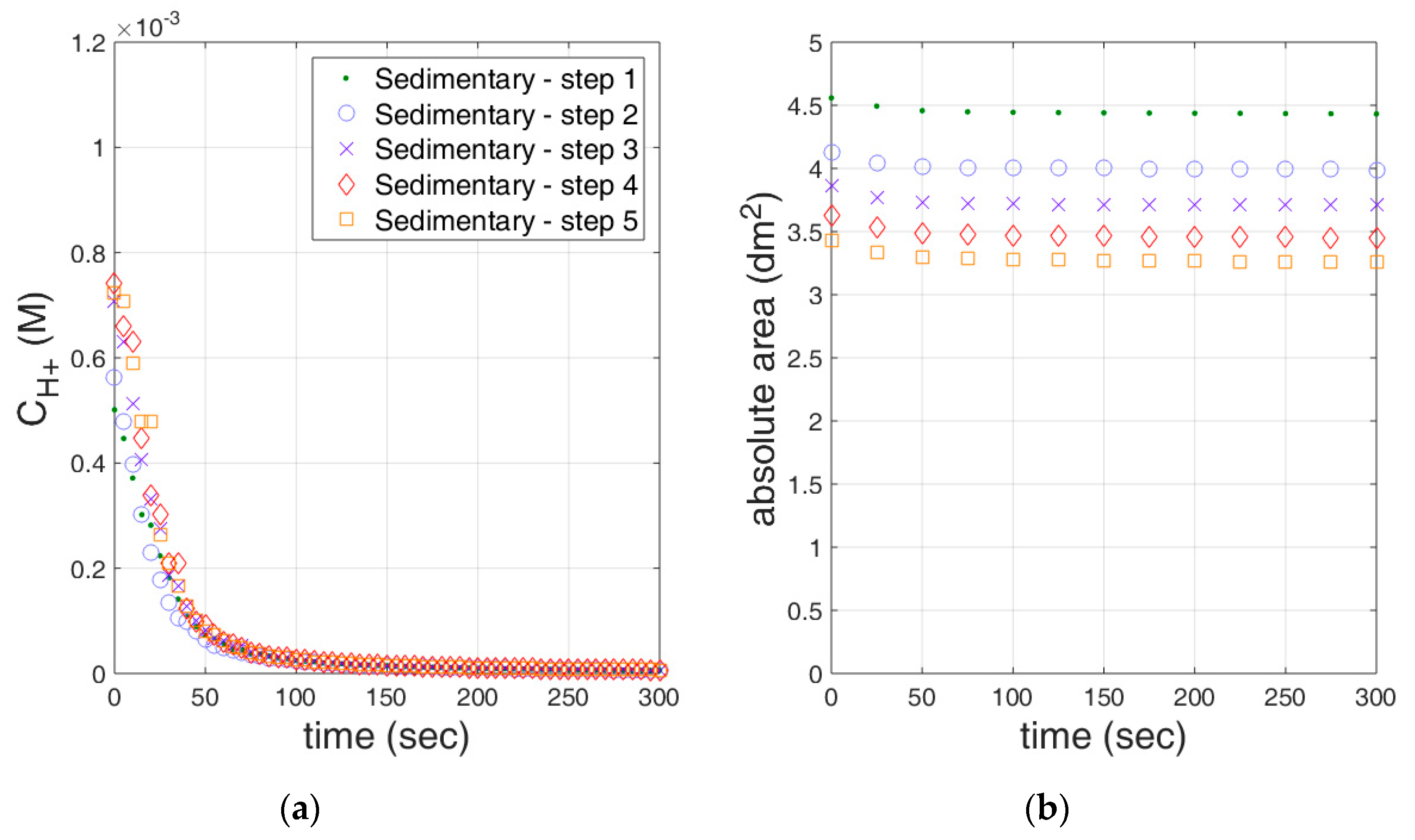
3.1. Limestone Analysis

The metamorphic limestone tested had a higher degree of crystals and a much less porous surface. In fact, our previous investigations on this kind of sample [30] demonstrated that the sedimentary limestone had around ten times more surface in comparison with the metamorphic one. However, it is also demonstrated that the effective surface actually used during the reactions can be very different because of surface-liquid interactions such as zeta potential [31,32] and surface tension [20,33,34]. Figure 2 gives a precise visual of the sample differences between the two kinds of limestone. As can be noticed, the crystallinity of the metamorphic limestone is greater than the sedimentary calcite; as a matter of fact, this sample has recrystallized in the form of marble during the Svecofennian orogeny. It is reported that this limestone was formed at temperature of around 800℃ and a pressure of five kilo bar [35]. Then, the metamorphic limestone has a higher degree of compaction with respect to the sedimentary one. The pores, edges, and corners and the superficial defects observed on the surface of the sedimentary sample point to a remarkable higher rugosity in comparison with the metamorphic sample, which seems to have a smoother grain surface. To some extent, this fact explains the difference in reactivity between the two kinds of limestone [36], observed in Section 3.2.

Table 2. Sample type, density, CaCO₃ content, and composition (wt %) given by X-Ray Fluorescence (XRF).

Sample	ρ (kg/m3)	CaCO3 wt %	CaO wt %	Al2O3 wt %	SiO2 wt %	MgO wt %
Metamorphic Limestone	2720	98.5	54.5	0.13	0.5	0.59
Sedimentary Limestone	2703	99.1	55.2	0.01	0.05	0.32

gives more information regarding the composition and density for the samples tested. The characterization refers to samples with a typical density for calcium carbonate samples with a low content of impurities, especially Mg and Al, whose presence is known to alter the reactivity of calcite toward dissolution and crystallization [37,38].

The PSD has been measured online during the course of the tests; the measures are carried out every 30 s for each step and the specific surface area, along with the PSD, is evaluated directly by the laser diffractometer by means of the Fraunhofer theory. The Fraunhofer approximation can be used when the particles are larger than 25 μm, since commonly, the laser beam employed has a wavelength of 0.63 μm. In fact, when a laser beam passes through a suspension of particles, the diffraction angle is inversely proportional to the particle diameter [39]. The Fraunhofer theory has been applied in this work, measuring the PSD by laser diffraction. Figure 3 and Figure 4 demonstrate the PSD for the first measure done at each titration step for the sedimentary and metamorphic samples, respectively.

Regarding the dissolution rate of limestone samples, the variation of the hydrogen ion concentration is determined from the pH register over time. The absolute contact area is determined by the conversion of the PSD measurements to a specific surface area and then multiplying this value by the undissolved calcium carbonate mass, which is obtained by mass balance based on the consumption of hydrogen. Figure 5 and Figure 6 report the hydrogen ion concentration and the absolute area time series for each step for the metamorphic and the sedimentary samples, respectively. The conversion of hydrogen ions is almost complete after 5 min, which is greater than 97%, while the calcium carbonate conversion is observed to be lower than 5% for each step. Except for the initial part, the absolute contact area remains approximately constant. This observation could be explained by the fact that most of the conversion of the hydrochloric acid takes place within the first minute, and the PSD does not change during the whole set of experiments.

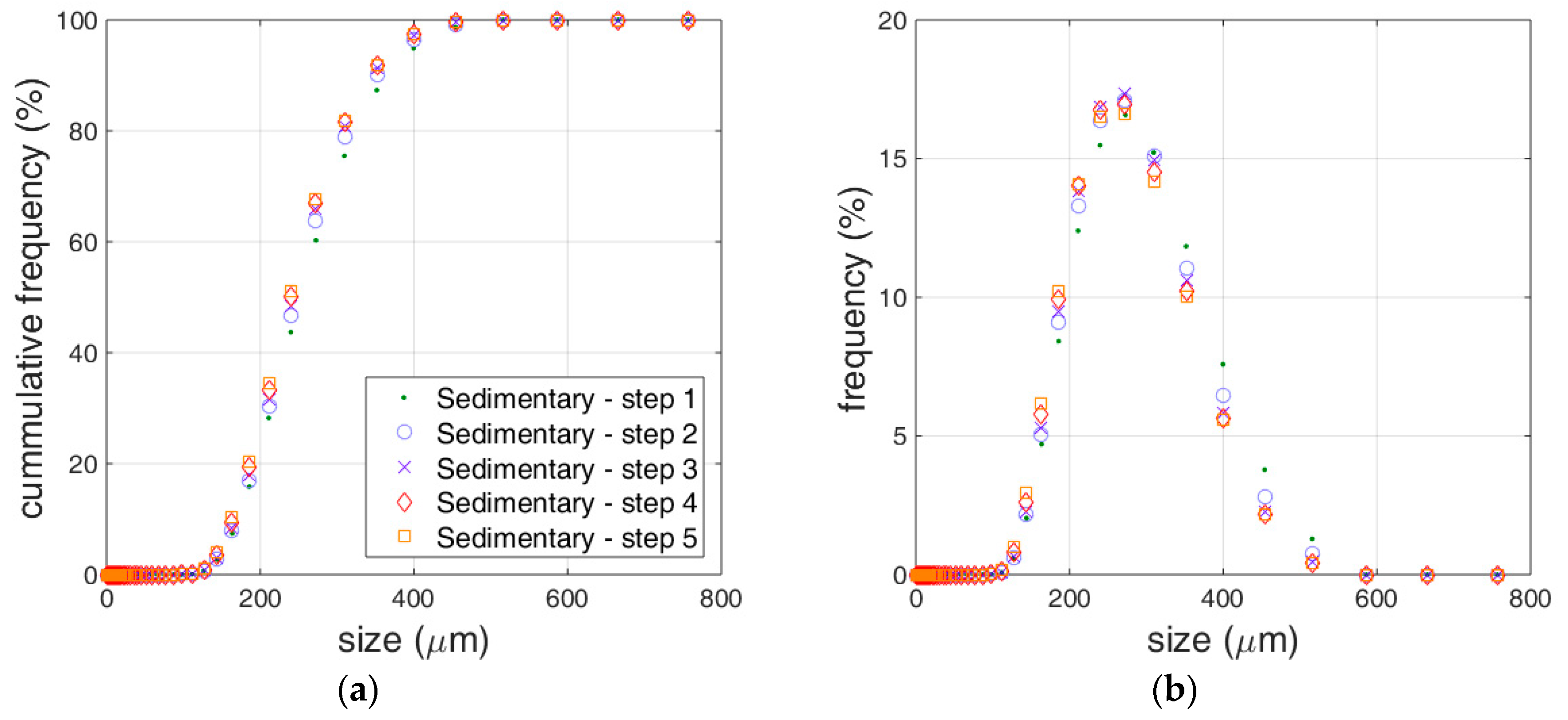
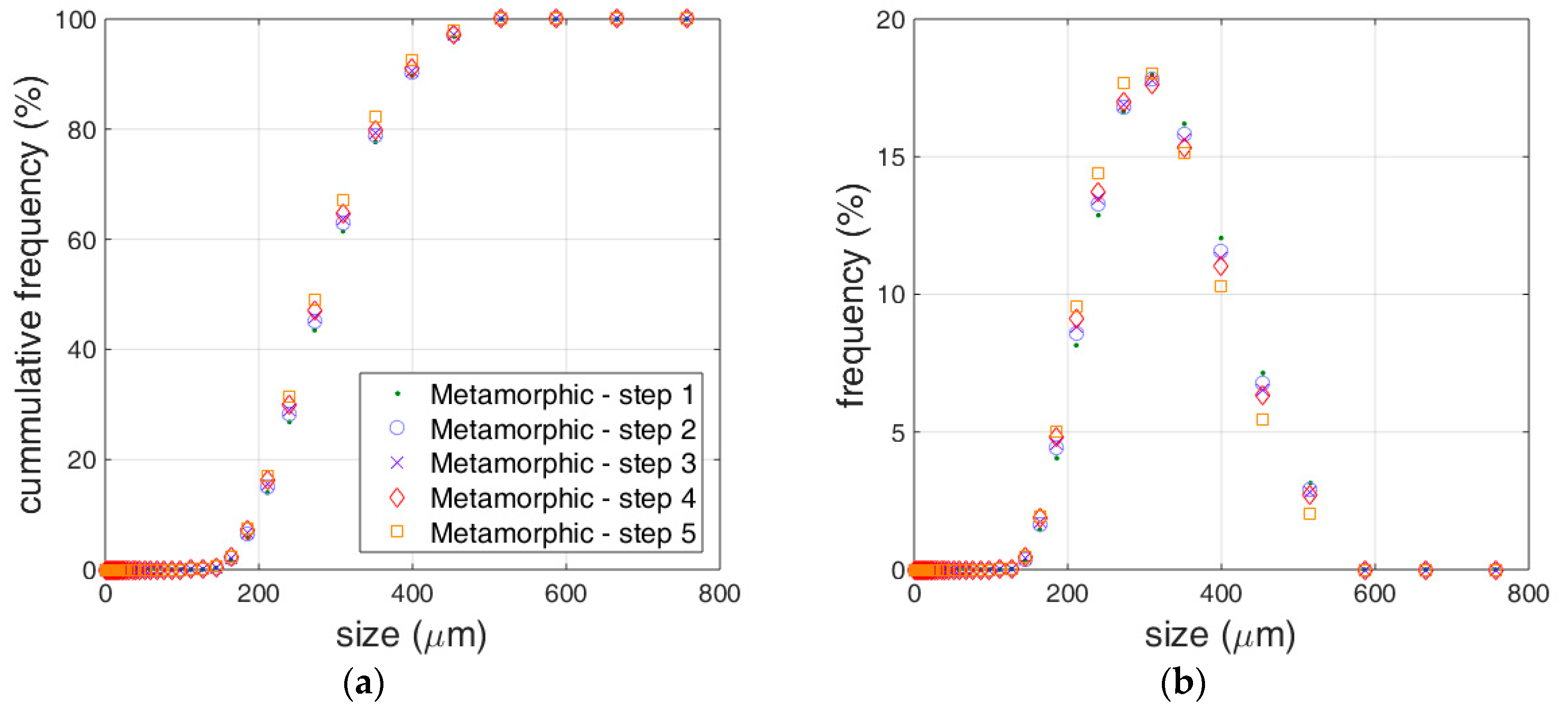
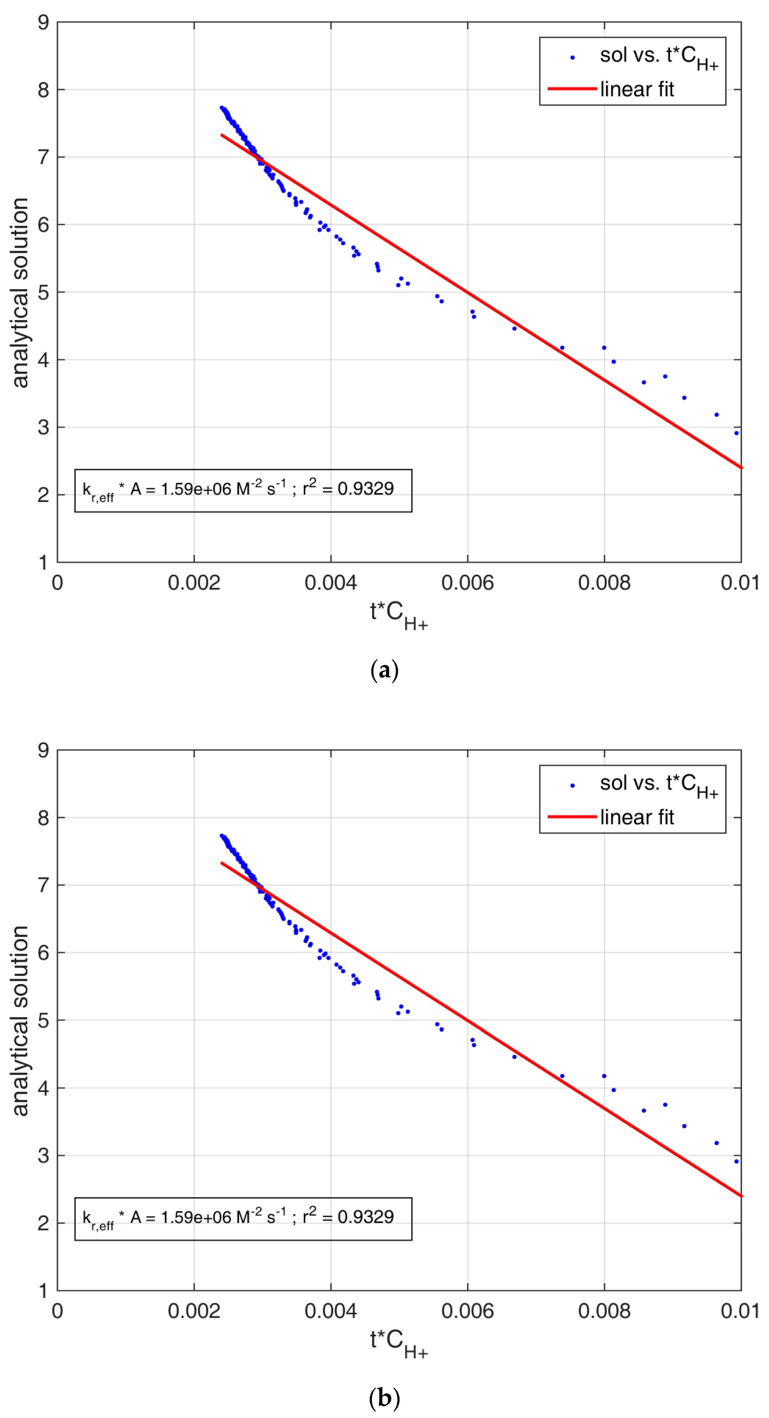
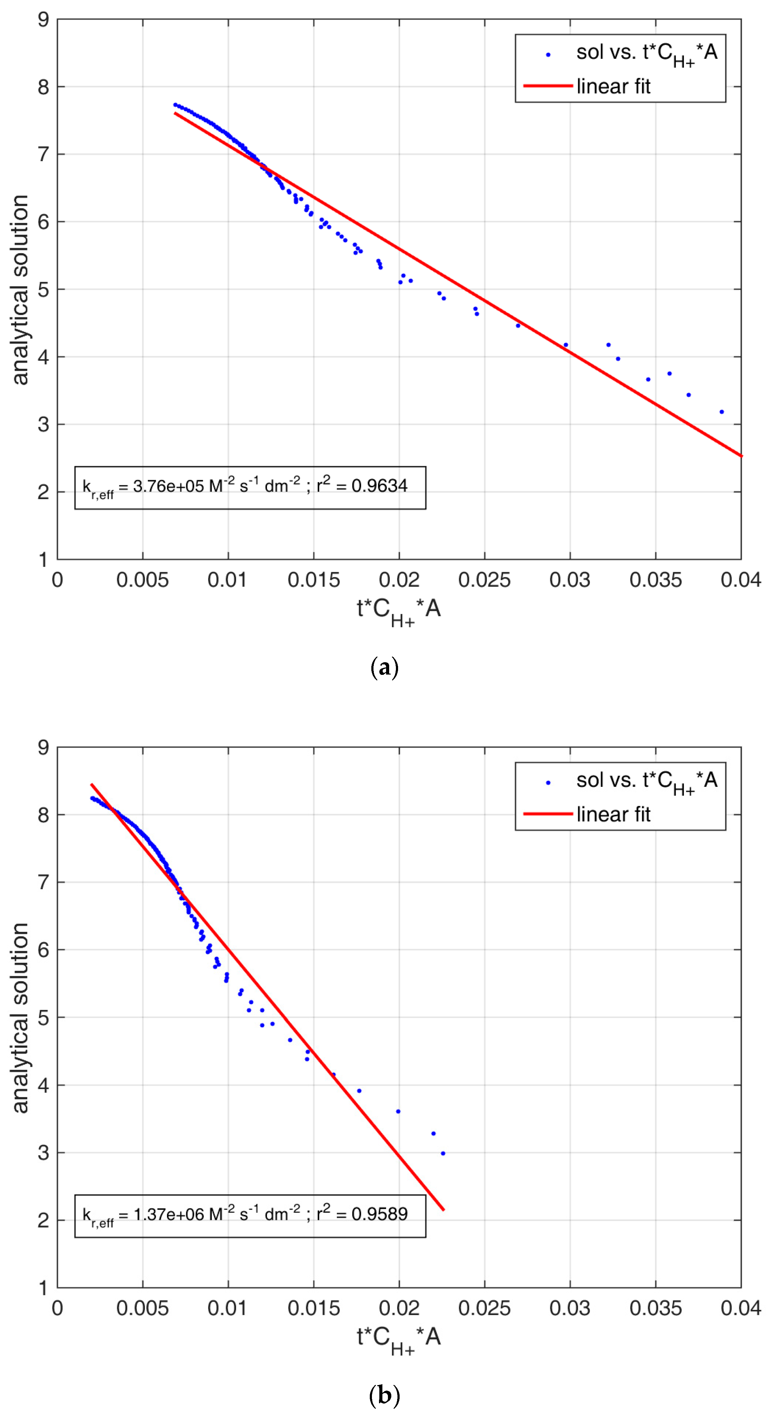
3.2. Reactivity Estimation of Limestone

Experiments of acidic dissolution were conducted on two different types of limestone, sedimentary and metamorphic, which were both quite pure in terms of CaCO₃ content. The rotating electrode experiments of Lund et al. (1975) [5] on calcite dissolution in hydrochloric acid solutions suggest that at low pH, the reaction can be considered irreversible, and the absorption of hydron over the solid calcite surface and subsequent reaction of the adsorbed hydron with the solid calcite matrix is the main reaction mechanism during the acidic dissolution of calcium carbonate. These facts are later confirmed by Shiraki et al. (2000) using Atomic Force Microscopy [40]. Therefore, from the model expressed in Equation (25), which is derived from mass balance considerations only, the parameter k’ will necessarily depend upon the activity of the adsorbed hydrogen ion on the calcite particle surface [41] ${\theta }_{H+}{C}_{H^{+}}^0$ as follows:

$$k^{\prime }=k_{\mathrm{p}}{\theta }_{H+}{C}_{H^{+}}^0$$

(26)

where ${\theta }_{H+}$ is the hydron activity coefficient on the surface of calcite, $k_p$ considers both the reactivity of the particle ($k_r$), and the interfacial mass transfer coefficient ($k_L$), which could be diffusional or convective depending on the fluid dynamics of the surrounding media. Thus, the parameter $k_p$ is affected by the chemical processes occurring at the surface, which in turn are influenced by the particle reactivity and the governing mass transfer mechanism. This could be diffusional or convective depending on the particle motion. The latter is well represented by the following Damköhler numbers [42]: $D{a}_I$ is defined as the ratio of the absolute reactivity $k_{r}A{C}_{H+}$ and the convective mass transfer coefficient ($k_{L,A}$); and $D{a}_{II}$ is defined as the ratio of the absolute reactivity and the diffusive mass transfer coefficient ($k_{L,D}$), which is defined as the ratio of the average ion diffusivity (D) and the mass transfer interfacial boundary layer thickness ($\delta$), which is itself an elusive parameter dependent on the instantaneous fluid dynamics surrounding each particle, and it will be subject of future works of this research group. So far, $\delta$ is estimated from correlations of the literature regarding mass transfer of solid particles submerged in turbulent liquid media [5,43]. The descriptor parameters of calcite dissolution dynamics in aqueous acidic media are presented within Table 3 in the context of this work.

The Reynolds number definition used here is that of agitated tanks, $Re=\rho {\varnothing }_A^{2}N/\mu$, where $\rho$ is the water density, ∅_A is the impeller diameter (0.03 m), N is the agitation rate (2300 rpm), and µ is the dynamic viscosity, which can be considered tend to have the same order of magnitude as water, since the solid loading is low and the shear rate is high [44]. The high value of the Reynolds number indicates a context of a fully developed turbulent flow, which points to the convective mass transfer as the dominant mechanism of calcite dissolution. This fact is confirmed by the value of $D{a}_I$, which in this context is several orders of magnitude lower than $D{a}_{II}$. When the solid motion is rapid enough, as in this case, $D{a}_I$ << $D{a}_{II}$, and it turns out that ${\theta }_{H+}$ is proportional to the $C_{H^{+}}$ of the bulk. Therefore, by averaging the characteristic times of each involved process, k_p stands as [2,45]:

$$\frac{{\theta }_{H+}{C}_{H^{+}}^0}{k_{\mathrm{p}}}=\frac{{\left(C_{H^{+}}^0\right)}^2}{k_{r,eff}}+\frac{1}{\delta }\left(\frac{1}{k_{L,A}}+\frac{1}{k_{L,D}}\right)=\frac{1}{k_{r,eff}}\left(1+D{a}_I+D{a}_{II}\right)$$

(27)

Thus, the right-hand side of Equation (27) results as $k_{r,eff}·C_{H^{+}}·A·t$, where $k_{r,eff}$ is a lumped reactivity constant that includes the influence of mass transfer and the proportionality between $C_{H^{+}}$ to ${\theta }_{H+}$.

Figure 7 shows the relation of the left hand term of Equation (27) with $C_{H^{+}}·t$. The average slope of the curve can be considered as the grouped product of the effective reactivity constant by the mean contact area. It is important to remark that in a fully developed turbulent flow such as this, the fluctuations at the fluid element scale of mass transfer rates within the system are the main source of errors. In this context, the surprising suitability of the linear fit shows that the initial variation of Solid-liquid contact area has little effect on the hypothesis of the constant surface area, which can be accepted, at least in the context of the presented experiments.

Table 3. Relevant physical parameters for the description of calcium carbonate particles dissolution in turbulent media.

Quantity	Symbol	Units	Min Value	Median Value	Max Value	Reference
Reynolds number (agitated tank)	Re	none		42,000		This Work
Convective mass transfer coefficient	$k_{L,A}$	10−3 dm/s	0.01	2	12	[2,43]
Limestone particle size	dp	10−6 m	150	320	500	This Work
Solid calcite concentration	$C_S$	g/L	2	3	5	This Work
Calcite absolute contact area	A	dm2	3	4	5	This Work
Conductivity (local)	σ	mS/cm2	0.4	100	105	[46]
Hydron concentration	$C_{H+}$	mol/L	10−6	6 × 10−6	2 × 10−3	This Work
Hydron surface activity coefficient	${\theta }_{H+}$	none	0	0.2	1	[2,47,48]
Hydron ion diffusivity in water	$D_{H+}$	10−5 cm2 s−1		9.3		[2,46]
Hydroxide anion diffusivity in water	$D_{OH-}$	10−5 cm2 s−1		5.273		[46]
Hydrogen Carbonate ion diffusivity in water	$D_{HC{O}_3-}$	10−5 cm2 s−1		1.185		[46]
Carbonate ion diffusivity in water	$D_{\frac{1}{2}C{O}_{3}2-}$	10−5 cm2 s−1		0.923		[46]
Calcium ion diffusivity in water	$D_{\frac{1}{2}Ca2+}$	10−5 cm2 s−1	0.79	0.792	0.84	[2,46]
Magnesium ion diffusivity in water	$D_{\frac{1}{2}Mg2+}$	10−5 cm2 s−1		0.706		[46]
Boundary layer thickness (mass transfer)	δ	10−5 m	1	2.4	5	[5,43]
Diffusive mass transfer coefficient	$k_{L,D}$	10−3 dm/s	0.14	2.8	9.3	This Work [2]
Effective reactivity parameter	$k_r{}_{,eff}$	M−2 dm−2 s−1	105	106	107	This work [2,41]
First Damköhler number	$D{a}_I$	none	104	106	109	This work
Second Damköhler number	$D{a}_{II}$	none	30	300	3000	This work

Table 3. Relevant physical parameters for the description of calcium carbonate particles dissolution in turbulent media.

Quantity	Symbol	Units	Min Value	Median Value	Max Value	Reference
Reynolds number (agitated tank)	Re	none		42,000		This Work
Convective mass transfer coefficient	$k_{L,A}$	10−3 dm/s	0.01	2	12	[2,43]
Limestone particle size	dp	10−6 m	150	320	500	This Work
Solid calcite concentration	$C_S$	g/L	2	3	5	This Work
Calcite absolute contact area	A	dm2	3	4	5	This Work
Conductivity (local)	σ	mS/cm2	0.4	100	105	[46]
Hydron concentration	$C_{H+}$	mol/L	10−6	6 × 10−6	2 × 10−3	This Work
Hydron surface activity coefficient	${\theta }_{H+}$	none	0	0.2	1	[2,47,48]
Hydron ion diffusivity in water	$D_{H+}$	10−5 cm2 s−1		9.3		[2,46]
Hydroxide anion diffusivity in water	$D_{OH-}$	10−5 cm2 s−1		5.273		[46]
Hydrogen Carbonate ion diffusivity in water	$D_{HC{O}_3-}$	10−5 cm2 s−1		1.185		[46]
Carbonate ion diffusivity in water	$D_{\frac{1}{2}C{O}_{3}2-}$	10−5 cm2 s−1		0.923		[46]
Calcium ion diffusivity in water	$D_{\frac{1}{2}Ca2+}$	10−5 cm2 s−1	0.79	0.792	0.84	[2,46]
Magnesium ion diffusivity in water	$D_{\frac{1}{2}Mg2+}$	10−5 cm2 s−1		0.706		[46]
Boundary layer thickness (mass transfer)	δ	10−5 m	1	2.4	5	[5,43]
Diffusive mass transfer coefficient	$k_{L,D}$	10−3 dm/s	0.14	2.8	9.3	This Work [2]
Effective reactivity parameter	$k_r{}_{,eff}$	M−2 dm−2 s−1	105	106	107	This work [2,41]
First Damköhler number	$D{a}_I$	none	104	106	109	This work
Second Damköhler number	$D{a}_{II}$	none	30	300	3000	This work

Figure 8 shows the relation of the left hand term of Equation (25) and $C_{H^{+}}$∙A∙t, considering not only the variation of $C_{H^{+}}$ in time but also the variation of surface area calculated from diffractive measurements. Despite the small change observed in the PSD measurements and absolute contact area, the linear correlation improves significantly when the time variation of the surface area is considered. The slope of the curve is an effective measure of the calcium carbonate reactivity at the surface of the limestone particles. Dividing the slope of the curve by the initial hydrogen concentration, we obtain k_r,eff.

It can be seen that in both Figure 7 and Figure 8, a linear relationship stands in a satisfactory agreement. While conserving an acceptable linear correlation, the k_r,eff of each run varies even within the same experimental conditions of agitation, which can be explained by the variability in the local conductivity of the dissolving media. The surface activity of the hydrogen ion ${\theta }_{H+}$ is closely related to the ionic mobility of the nearby media [34,47]. Carletti et al. (2016) [9] report the non-uniformity of conductivity for the very same system, which is measured by Electrical Resistance Tomography. Then, the fluctuations of local conductivity at the element of fluid level play a major role explaining the errors of the linear fitting observed in Figure 7 and Figure 8. Recent studies over calcite dissolution rates indicate that its active surface is not homogeneous but rather intricately distributed over the exposed layer [49]. A stochastic pattern of superficial detachment is expected during the process that is complex enough to ascertain that the reactivity of the particles is not constant; nevertheless, in practice, the observed reactivity is a robust statistical estimator due to numerical compensation, as shown in

Table 4. Results of the model fit on the experimental results.

Experiment	kr,eff A (107 M−2 s−1)	Goodness of Fit (r2)	Averaged Contact Area (dm2)	kr,eff (107 M−2 dm−2 s−1)	Goodness of Fit (r2)
Metamorphic_step1	0.159 ± 0.008	0.9329	3.76 ± 0.33	0.038 ± 0.001	0.9634
Metamorphic_step2	0.129 ± 0.009	0.8835	3.78 ± 0.31	0.031 ± 0.002	0.9216
Metamorphic_step3	0.112 ± 0.008	0.8683	3.72 ± 0.38	0.027 ± 0.002	0.9126
Metamorphic_step4	0.132 ± 0.010	0.8719	3.80 ± 0.28	0.032 ± 0.002	0.9085
Metamorphic_step5	0.109 ± 0.008	0.8512	3.74 ± 0.36	0.026 ± 0.002	0.8935
Sedimentary_step1	0.636 ± 0.034	0.9020	3.45 ± 0.70	0.137 ± 0.005	0.9589
Sedimentary_step2	1.018 ± 0.057	0.9124	3.74 ± 0.35	0.223 ± 0.008	0.9619
Sedimentary_step3	0.409 ± 0.032	0.8527	3.78 ± 0.30	0.097 ± 0.006	0.9109
Sedimentary_step4	0.327 ± 0.030	0.8035	3.75 ± 0.34	0.079 ± 0.006	0.8730
Sedimentary_step5	0.428 ± 0.035	0.8329	3.74 ± 0.36	0.101 ± 0.006	0.9062

. The actual reactive portion of the outer layer rounds is reported as 20% of the grain surface [48], which depends upon the composition of the bulk (especially the conductivity of the medium), the instantaneous size distribution of the particles, the interfacial tension, and the agitation conditions [2,33,37].

The values determined in this work are within the same order of magnitude as the reported experimentally by Sjöberg and Rickard (1984) [41] and later calculated by Letterman (1995) [2] in similar conditions. The difference arising from the sample origin is remarkable and up to four times higher in the case of the sedimentary rough sample with respect to the metamorphic smooth sample.

4. Discussion

Multiphase transport phenomena represent one of the most important study areas in the process industry. A detailed mathematical modeling allows reducing the computational time regarding the reactors’ design and operations. As a matter of fact, as it was described within this article, the common case presented is that mass balances are described by differential equations where some variables involved are measured during experiments, while additional parameters have to be retrieved. For instance, these parameters could be the mass transfer coefficient and the diffusivity of the dissolving element. Those parameters could be evaluated by implementing a software procedure to obtain a suitable regression coefficient, and their value could be obtained by iteration. One example is the Levenberg-Marquardt method.

If diverse mathematical models should be tested, analytical solutions significantly speed up this process, especially in the case when iterative methods are used. For instance, when experimental data are available on the dissolved concentrations vs. time and the goal is to find the correct value for the mass transfer coefficient.

The surface area of a particle is crucial to the dissolution rate. Particles are not commonly spherical in nature, and steady-state conditions are not always the case in practical implementations. The importance of taking the particle shape into account lies in the fact that spheres have a low surface to volume ratio, and when a particle has an irregular shape very different to a sphere, the surface to volume ratio will be much greater.

Researchers take into consideration a shape factor in relation to their volume, and this treatment complicates the mathematical models provided. The solutions presented in this paper are giving general methods for the shrinking model, and they can be expanded to non-spherical particles with diverse shape factors as well. The assumption considered here is that the component of interest is dissolving in a well-mixed batch system and that particles are completely suspended.

Solid dissolution in liquids is particularly important if we consider wet Flue Gas Desulfurization or carbon dioxide capture, where limestone dissolution plays a fundamental role. However, this can be extended to many applications, which go from the chemical engineering field of process design to the pharmaceutical industry.

The balance presented by Equation (3) states that the dissolution rate for the solid phase is directly proportional to its concentration and also proportional to the concentration of the dissolved element in the liquid phase. Most importantly, the dissolution is affected by the shape of the particles, and this is considered as part of the power coefficient of the concentration value.

This is not a new approach; analyzing the proportionalities in terms of the dimensions applied represents one of the starting steps to derive valuable information. In the literature, there are similar models applied to the dissolution of solids [26,27,28]. Nonetheless, no analytical solution of this form has been presented before.

The surface of the reaction is changing with time, and it will be decreasing eventually, although the specific surface area increases even if this is not always the case [10,33]. On the other hand, the shape factor for this kind of particle might not be fixed, and it could vary from the case presented here, which could also be studied further.

The experimental results provided here demonstrate examples of applications for the analytical solution given. The model was successfully verified within all the experimental datasets analyzed. Furthermore, the parameters shown in Table 4, which were obtained from fitting the model, are in accordance with the previous dedicated literature. They are also a robust measure of the limestone’s reactivity, which can be used for the comparison of raw materials with different geological backgrounds and sizes. We observed a fine quality of the linear fit, which is represented by the coefficient of determination r², which in none of the dozens of experiments we carried out is observed lower than 0.85. Actually, for these samples, the average determination coefficient is 0.92 +/− 0.06. As a matter of fact, the fitting of this model with experimental data for the case of limestone dissolution is rather complicated, considering the complexity of the interfacial mass transfer in turbulent media, and it is a great step forward toward understanding the limestone dissolution in detail, which is the key for the optimization, scaling up, and de-risking of flue gas desulfurization.

5. Conclusions

Particles are not commonly spherical in nature, and steady-state conditions are not always the case in practical implementations. The importance of taking the particle shape into account lies in the fact that spheres have a low surface to volume ratio, and when a particle has an irregular shape that is very different from a sphere, the surface to volume ratio will be much greater. The surface area of a particle is crucial to the dissolution rate.

Researchers take into consideration a shape factor in relation to their volume, and this treatment complicates the mathematical models provided. The solutions presented in this paper are giving general clarifications for the shrinking model, but they can be expanded to non-spherical particles and with diverse shape factors. The assumption considered here is that the component of interest is dissolving in a well-mixed batch system and that particles are completely suspended.

This simple approach keeps most of the dominant underlying dynamics, and its parameters provide a robust prediction for the reactivity of the limestone particles. This information can be used for modeling global reactor behavior without the need for time-consuming simulations. In addition, data acquired can be utilized to move our understanding to a more quantitative and predictive level, which is needed for reducing the risk of scale-up and for design of the next generation of reactors and processes.

Nevertheless, in this framework, the goal here is to demonstrate the analytical solution of the models presented, and this represents a novelty in this sense. The application of these results could open further comprehension of additional process aspects beyond the estimated contact area; for example, bulk ion mobility and interfacial free energy represent a larger scope that should be investigated in additional studies.

References

1. Levich, V.G. Physicochemical Hydrodynamics; Prentice Hall: Upper Saddle River, NJ, USA, 1962; ISBN 0-13-674440-0. [Google Scholar]
2. Letterman, R.D. Calcium Carbonate Dissolution Rate in Limestone Contactors | Project Summary: Calcium Carbonate Dissolution Rate in Limestone Contactors; U.S. Environmental Protection Agency: Washington, DC, USA, 1995.
3. Hattori, Y.; Haruna, Y.; Otsuka, M. Dissolution process analysis using model-free Noyes-Whitney integral equation. Colloids Surf. B Biointerfaces 2013, 102, 227–231. [Google Scholar] [CrossRef] [PubMed]
4. Aris, R. On shape factors for irregular particles—I: The steady state problem. Diffusion and reaction. Chem. Eng. Sci. 1957, 6, 262–268. [Google Scholar] [CrossRef]
5. Lund, K.; Fogler, H.S.; McCune, C.C.; Ault, J.W. Acidization—II. The dissolution of calcite in hydrochloric acid. Chem. Eng. Sci. 1975, 30, 825–835. [Google Scholar] [CrossRef] [Green Version]
6. Gray, F.; Anabaraonye, B.; Shah, S.; Boek, E.; Crawshaw, J. Chemical mechanisms of dissolution of calcite by HCl in porous media: Simulations and experiment. Adv. Water Resour. 2018, 121, 369–387. [Google Scholar] [CrossRef]
7. Mahulkar, A.V.; Gogate, P.R.; Pandit, A.B. Matching Chemistry with Chemical Engineering for Optimum Design and Performance of Pharmaceutical Processing. In Pharmaceutical Process Chemistry; John Wiley & Sons, Ltd.: Hoboken, NJ, USA, 2010; pp. 443–467. ISBN 978-3-527-63367-8. [Google Scholar]
8. Kartashev, A.L.; Kartasheva, M.A.; Terekhin, A.A. Mathematical Models of Dynamics Multiphase Flows in Complex Geometric Shape Channels. Procedia Eng. 2017, 206, 121–127. [Google Scholar] [CrossRef]
9. Carletti, C.; Montante, G.; De Blasio, C.; Paglianti, A. Liquid mixing dynamics in slurry stirred tanks based on electrical resistance tomography. Chem. Eng. Sci. 2016, 152, 478–487. [Google Scholar] [CrossRef]
10. De Blasio, C.; Carletti, C.; Lundell, A.; Visuri, V.-V.; Kokkonen, T.; Westerlund, T.; Fabritius, T.; Järvinen, M. Employing a step-wise titration method under semi-slow reaction regime for evaluating the reactivity of limestone and dolomite in acidic environment. Miner. Eng. 2016, 86, 43–58. [Google Scholar] [CrossRef]
11. De Blasio, C.; Carletti, C.; Westerlund, T.; Järvinen, M. On modeling the dissolution of sedimentary rocks in acidic environments. An overview of selected mathematical methods with presentation of a case study. J. Math. Chem. 2013, 51, 2120–2143. [Google Scholar] [CrossRef]
12. Organization of the Petroleum Exporting Countries, OPEC. World Oil Outlook 2040; OPEC: Vienna, Austria, 2018; ISBN 978-3-9503936-6-8. [Google Scholar]
13. World Bank World—Total Population 2008–2018. Available online: https://www.statista.com/statistics/805044/total-population-worldwide/ (accessed on 24 December 2019).
14. De Blasio, C. Introduction. In Fundamentals of Biofuels Engineering and Technology; Springer International Publishing: Basel, Switzerland, 2019; pp. 3–12. [Google Scholar]
15. Dudley, B. Proven coal reserves leading countries 2018. In BP Statistical Review of World Energy; Pureprint Group Limited: Uckfield, UK, 2019; p. 42. Available online: https://www.bp.com/content/dam/bp/business-sites/en/global/corporate/pdfs/energy-economics/statistical-review/bp-stats-review-2020-full-report.pdf (accessed on 22 November 2020).
16. ECN, The Netherlands Phyllis2—Database for Biomass and Waste. Available online: https://www.ecn.nl/phyllis2/ (accessed on 22 August 2018).
17. Huang, J.; Wang, H.; Zhong, Y.; Huang, J.; Fu, X.; Wang, L.; Teng, W. Growth and physiological response of an endangered tree, Horsfieldia hainanensis merr., to simulated sulfuric and nitric acid rain in southern China. Plant Physiol. Biochem. 2019, 144, 118–126. [Google Scholar] [CrossRef]
18. Srivastava, R.K.; Jozewicz, W.; Singer, C. SO2 scrubbing technologies: A review. Environ. Prog. 2001, 20, 219–228. [Google Scholar] [CrossRef]
19. Carletti, C.; De Blasio, C.; Mäkilä, E.; Salonen, J.; Westerlund, T. Optimization of a Wet Flue Gas Desulfurization Scrubber through Mathematical Modeling of Limestone Dissolution Experiments. Ind. Eng. Chem. Res. 2015, 54, 9783–9797. [Google Scholar] [CrossRef]
20. De Blasio, C.; Carletti, C.; Salonen, J.; Björklund-Sänkiaho, M. Ultrasonic Power to Enhance Limestone Dissolution in the Wet Flue Gas Desulfurization Process. Modeling and Results from Stepwise Titration Experiments. ChemEngineering 2018, 2, 53. [Google Scholar] [CrossRef] [Green Version]
21. Carletti, C.; De Blasio, C.; Miceli, M.; Pirone, R.; Westerlund, T. Ultrasonic enhanced limestone dissolution: Experimental and mathematical modeling. Chem. Eng. Process. Process Intensif. 2017, 118, 26–36. [Google Scholar] [CrossRef]
22. Molerus, O.; Latzel, W. Suspension of solid particles in agitated vessels—II. Archimedes numbers > 40, reliable prediction of minimum stirrer angular velocities. Chem. Eng. Sci. 1987, 42, 1431–1437. [Google Scholar] [CrossRef]
23. Plummer, L.N.; Wigley, T.M.L.; Parkhurst, D.L. The kinetics of calcite dissolution in CO2—water systems at 5 degrees to 60 degrees C and 0.0 to 1.0 atm CO2. Am. J. Sci. 1978, 278, 179–216. [Google Scholar] [CrossRef]
24. Ahlbeck, J.; Engman, T.; Fältén, S.; Vihma, M. Measuring the reactivity of limestone for wet flue-gas desulfurization. Chem. Eng. Sci. 1995, 50, 1081–1089. [Google Scholar] [CrossRef]
25. Levenspiel, O. Chemical Reaction Engineering, 3rd ed.; Wiley: Hoboken, NJ, USA, 1998; ISBN 0-471-25424-X. [Google Scholar]
26. Salmi, T.; Grénman, H.; Wärnå, J.; Murzin, D.Y. New modelling approach to liquid-solid reaction kinetics: From ideal particles to real particles. Chem. Eng. Res. Des. 2013, 91, 1876–1889. [Google Scholar] [CrossRef]
27. Russo, V.; Salmi, T.; Carletti, C.; Murzin, D.Y.; Westerlund, T.; Tesser, R.; Grénman, H. Application of an Extended Shrinking Film Model to Limestone Dissolution. Ind. Eng. Chem. Res. 2017, 56, 13254–13261. [Google Scholar] [CrossRef]
28. Salmi, T.; Grénman, H.; Wärnå, J.; Murzin, D.Y. Revisiting shrinking particle and product layer models for fluid-solid reactions—From ideal surfaces to real surfaces. Chem. Eng. Process. Process Intensif. 2011, 50, 1076–1084. [Google Scholar] [CrossRef]
29. Salmi, T.; Grénman, H.; Bernas, H.; Wärnå, J.; Murzin, D.Y. Mechanistic modelling of kinetics and mass transfer for a Solid-liquid system: Leaching of zinc with ferric iron. Chem. Eng. Sci. 2010, 65, 4460–4471. [Google Scholar] [CrossRef]
30. Carletti, C.; Grénman, H.; De Blasio, C.; Mäkilä, E.; Salonen, J.; Murzin, D.Y.; Salmi, T.; Westerlund, T. Revisiting the dissolution kinetics of limestone—Experimental analysis and modeling. J. Chem. Technol. Biotechnol. 2015, 91, 1517–1531. [Google Scholar] [CrossRef]
31. Otsuki, A.; Hayagan, N.L. Zeta potential of inorganic fine particle—Na-bentonite binder mixture systems. Electrophoresis 2020, 41, 1405–1412. [Google Scholar] [CrossRef] [PubMed]
32. Al Mahrouqi, D.; Vinogradov, J.; Jackson, M.D. Zeta potential of artificial and natural calcite in aqueous solution. Adv. Colloid Interface Sci. 2017, 240, 60–76. [Google Scholar] [CrossRef] [PubMed] [Green Version]
33. Rezaei Gomari, S.; Amrouche, F.; Santos, R.G.; Greenwell, H.C.; Cubillas, P. A New Framework to Quantify the Wetting Behaviour of Carbonate Rock Surfaces Based on the Relationship between Zeta Potential and Contact Angle. Energies 2020, 13, 993. [Google Scholar] [CrossRef] [Green Version]
34. Derkani, M.H.; Fletcher, A.J.; Fedorov, M.; Abdallah, W.; Sauerer, B.; Anderson, J.; Zhang, Z.J. Mechanisms of Surface Charge Modification of Carbonates in Aqueous Electrolyte Solutions. Colloids Interfaces 2019, 3, 62. [Google Scholar] [CrossRef] [Green Version]
35. Väisänen, M.; Hölttä, P. Structural and metamorphic evolution of the Turku migmatite complex, southwestern Finland. Geol. Surv. Finl. 2002, 71, 177–218. [Google Scholar] [CrossRef]
36. Bang, J.-H.; Song, K.; Park, S.; Jeon, C.; Lee, S.-W.; Kim, W. Effects of CO2 Bubble Size, CO2 Flow Rate and Calcium Source on the Size and Specific Surface Area of CaCO3 Particles. Energies 2015, 8, 12304–12313. [Google Scholar] [CrossRef] [Green Version]
37. Yuan, K.; Starchenko, V.; Lee, S.S.; De Andrade, V.; Gursoy, D.; Sturchio, N.C.; Fenter, P. Mapping Three-dimensional Dissolution Rates of Calcite Microcrystals: Effects of Surface Curvature and Dissolved Metal Ions. ACS Earth Space Chem. 2019, 3, 833–843. [Google Scholar] [CrossRef]
38. Davis, K.J.; Dove, P.M.; Yoreo, J.J.D. The Role of Mg2+ as an Impurity in Calcite Growth. Science 2000, 290, 1134–1137. [Google Scholar] [CrossRef]
39. Rhodes, M. Introduction to Particle Technology, 2nd ed.; Wiley: Hoboken, NJ, USA, 2008; ISBN 978-0-470-01427-1. [Google Scholar]
40. Shiraki, R.; Rock, P.A.; Casey, W.H. Dissolution Kinetics of Calcite in 0.1 M NaCl Solution at Room Temperature: An Atomic Force Microscopic (AFM) Study. Aquat. Geochem. 2000, 6, 87–108. [Google Scholar] [CrossRef]
41. Sjöberg, E.L.; Rickard, D.T. Calcite dissolution kinetics: Surface speciation and the origin of the variable pH dependence. Chem. Geol. 1984, 42, 119–136. [Google Scholar] [CrossRef]
42. Fogler, H.S. Elements of Chemical Reaction Engineering, 5th ed.; Prentice Hall: Boston, MA, USA, 2016; ISBN 978-0-13-388751-8. [Google Scholar]
43. Blasio, C.D.; Mäkilä, E.; Westerlund, T. Use of carbonate rocks for flue gas desulfurization: Reactive dissolution of limestone particles. Appl. Energy 2012, 90, 175–181. [Google Scholar] [CrossRef]
44. Nascimento, D.R.; Oliveira, B.R.; Saide, V.G.P.; Magalhães, S.C.; Scheid, C.M.; Calçada, L.A. Effects of particle-size distribution and solid additives in the apparent viscosity of drilling fluids. J. Pet. Sci. Eng. 2019, 182, 106275. [Google Scholar] [CrossRef]
45. Yamauchi, V.; Tanaka, K.; Hattori, K.; Kondo, M.; Ukawa, N. Remineralization of desalinated water by limestone dissolution filter. Desalination 1987, 66, 365–383. [Google Scholar] [CrossRef]
46. Lide, D.R. CRC Handbook of Chemistry and Physics: A Ready-Reference Book of Chemical and Physical Data; CRC Press: Boca Raton, FL, USA, 2017; ISBN 978-1-4987-5428-6. [Google Scholar]
47. Steefel, C.I.; Maher, K. Fluid-Rock Interaction: A Reactive Transport Approach. Rev. Mineral. Geochem. 2009, 70, 485–532. [Google Scholar] [CrossRef]
48. Brand, A.S.; Feng, P.; Bullard, J.W. Calcite dissolution rate spectra measured by in situ digital holographic microscopy. Geochim. Cosmochim. Acta 2017, 213, 317–329. [Google Scholar] [CrossRef]
49. Fischer, C.; Arvidson, R.S.; Lüttge, A. How predictable are dissolution rates of crystalline material? Geochim. Cosmochim. Acta 2012, 98, 177–185. [Google Scholar] [CrossRef]
Figure 1. Experimental set-up for limestone dissolutions assays. In the figure, the Malvern Mastersizer 3000 is shown on the left side with its Hydro Unit. Temperature and pH are measured by a pH meter, and the sensor is connected to a pH-controlling unit (center). For experiments where the pH is required to be constant, a peristaltic pump with a scale (right side) can be used.
Energies 13 06164 g001
Figure 2. SEM images for sedimentary limestone (a) and metamorphic limestone (b). Åbo Akademi University.
Energies 13 06164 g002
Figure 3. Sedimentary limestone: cumulative size distribution (a) and size frequency density (b).
Energies 13 06164 g003
Figure 4. Metamorphic limestone: cumulative size distribution (a) and size frequency density (b).
Energies 13 06164 g004
Figure 5. Hydrogen ion concentration (a) and absolute contact area (b) time series for the metamorphic limestone sample registered for each step.
Energies 13 06164 g005
Figure 6. Hydrogen ion concentration (a) and absolute contact area (b) time series for the sedimentary limestone sample registered for each step. The sampling time period of pH (therefore C H + ) was 5 s and the area measurement frequency was every 30 s.
Energies 13 06164 g006
Figure 7. Correlation between the left-hand side of Equation (25) and t· C H + for the metamorphic (a) and sedimentary (b) limestone samples. The absolute value of the regression slope is reported in the figure; it can be considered as the mean area multiplied by an estimator of the effective reactivity.
Energies 13 06164 g007
Figure 8. Correlation between the left-hand side of Equation (25) and t· ( C H + ) A for the metamorphic (a) and sedimentary (b) limestone samples. The absolute value of the regression slope is reported in figure. This represents an estimator of the effective reactivity.
Energies 13 06164 g008