Article

A Stacked Denoising Sparse Autoencoder Based Fault Early Warning Method for Feedwater Heater Performance Degradation

1
Harbin Institute of Technology, Harbin 150001, Heilongjiang, China
2
Science and Technology on Thermal Energy and Power Laboratory, Wuhan 430205, Hubei, China
*
Author to whom correspondence should be addressed.
Energies 2020, 13(22), 6061; https://doi.org/10.3390/en13226061
Submission received: 15 October 2020 / Revised: 17 November 2020 / Accepted: 17 November 2020 / Published: 19 November 2020
(This article belongs to the Special Issue Machine Learning Applications in Power System Condition Monitoring)

Abstract

:
Power grid operation faces severe challenges with the increasing integration of intermittent renewable energies. Hence the steam turbine, which mainly undertakes the task of frequency regulation and peak shaving, always operates under off-design conditions to meet the accommodation demand. This would affect the operation economy and exacerbate the ullage of equipment. The feedwater heater (FWH) plays an important role in unit, whose timely fault early warning is significant in improving the operational reliability of unit. Therefore, this paper proposes a stacked denoising sparse autoencoder (SDSAE) based fault early warning method for FWH. Firstly, the concept of a frequent pattern model is proposed as an indicator of FWH performance evaluation. Then, an SDSAE- back-propagation (BP) based method is introduced to achieve self-adaptive feature reduction and depict nonlinear properties of frequent pattern modeling. By experimenting with actual data, the feasibility and validity of the proposed method are verified. Its detection accuracy reaches 99.58% and 100% for normal and fault data, respectively. Finally, competitive experiments prove the necessity of feature reduction and the superiority of SDSAE based feature reduction compared with traditional methods. This paper puts forward a precise and effective method to serve for FWH fault early warning and refines the key issues to inspire later researchers.

Graphical Abstract

1. Introduction

The utilization of renewable energies is regarded as a promising way to satisfy energy demand and reduce carbon emissions. With the gradual expansion of installed capacity, they have become an important part in power generation. However, the growing accommodation ratio of intermittent renewable energy brings great challenges to power grid stability and security. Under this context, the steam turbine has an increasingly prominent role in peak shaving and frequency modulating. The safe and economic operation of the steam turbine are influenced due to long-time operation under off-design conditions and frequent load changes [1,2]. Feedwater heating systems play a critical role in the steam turbine which is of great significance in energy saving [3,4,5]. The FWH often works in severe conditions of high temperature and pressure [6]. Additionally, the impact of continuously alternate changing temperature leads to scaling, blockage and even rupture of the FWH U-tube pipe, and may cause a chain reaction in the heating system [7]. Hence, a sufficient method for FWH performance evaluation and fault early warning is urgently needed [8], which is of great practical value as it will preclude catastrophic failures, diminish operating costs and contribute to the enhancement of intelligent operation and maintenance level.
In previous studies, researchers have obtained many achievements through various methods. Generally, these methods can be classified into two major categories: mechanism-model-based methods and data-driven based methods. Barszcz et al. [9,10] propose a first-principle four-volume model of FWH in which model parameters are adjusted through operational data and performance indicators are proposed. Zhao et al. [11] use GSE software to build a coal-fired power plant simulation model including FWH. Chen et al. [12] apply the dominant factor method to monitor the regenerative system’s performance. Although the structure of the FWH is simple, the heat transfer process is complex and multiform, which makes it hard to establish sufficiently accurate physical models for performance monitoring. Hence, the fault early warning performance of mechanism-model-based methods is limited to some extent due to the model accuracy.
Data-driven based methods mine the relationship between data and achieve fault early warning without introduction of physical modeling error. Jiang et al. [13] propose a data reconciliation-based approach for fault detection, but the accuracy is not good enough. Wang et al. [14] propose a nearest prototype classifier combined with a hybrid particle swarm optimization algorithm to classify different types of fault. Li et al. [15] present a fault diagnosis method based on the enhanced group method of data handling. Kang et al. [16] introduce a fuzzy inference system to diagnose performance degradation for FWH. Ma et al. [17] propose a hybrid method of artificial neural networks and optimal zoom search for recognizing varying degrees of faults. In references [18,19], a two-stage back-propagation network and radial basis function neural network are adopted for fault diagnosis, respectively. Heo et al. [20] develop a diagnosis model using a feed-forward neural network to reveal the correlation between thermal performance indices and leakage conditions. Garcia et al. [21] use neural networks to identify the heat transfer capacity of the heater. Radhakrishnan et al. [22] use adaptive neural networks to predict the heat transfer coefficient and the fouling rate of the heat exchanger.
Previous studies are overly concerned with adopting advanced methods to identify fault characteristics and avoid the limitation from physical modeling error, whereas these characteristics mostly rely on fault data analysis and expert knowledge. It must be noted that the fault data is rare and hard to obtain in practice. That is, the data sparsity problem is the challenge to obtain fault information. Moreover, the feature selection for depicting fault characteristics is quite different in previous studies [12,13,14,15,16,17,18,19,20,21,22]. For the same research object, there should be an optimal feature combination for fault early warning, but so far there is no systematic analysis from a scientific view.
To fill the gap and achieve the goal, this paper proposes a stacked denoising sparse autoencoder (SDSAE) based fault early warning method for FWH performance degradation. Firstly, the concept of frequent pattern model is proposed to depict FWH performance from the perspective of the fault mechanism. Then, considering the high coupling characteristics and nonlinear properties of FWH, SDSAE and back-propagation neural network (BPNN) are combined to achieve self-adaptive feature reduction and nonlinear characteristics expression for frequent pattern modeling. Via experiment with actual data, the feasibility and validity of the proposed method are verified and its detection accuracy reaches 99.58% and 100% for normal and fault data respectively. Moreover, the results of comparison experiments with different modeling methods demonstrate the necessity of feature reduction in FWH fault early warning, and the superiority of SDSAE in feature reduction over traditional methods.
The rest of this paper is organized as follows: Section 2 analyzes the key issues for FWH fault early warning and puts forward the concept of the frequent pattern model. Section 3 introduces the implementation process of the proposed SDSAE-BP-based frequent pattern model method. Section 4 conducts experiments with actual data and carries out competitive experiments as well as corresponding discussion. Section 5 concludes the paper and outlines future research orientations.

2. Key Issues of FWH Fault Early Warning

2.1. Traditional Method Analysis

In this paper, #2 high-pressure FWH of a typical 630 MW supercritical coal-fired unit is selected as the research object. The reason for selecting #2 FWH is as follows. Although #1 high-pressure FWH has the most obvious impact on economy, #2 FWH, which obtains the inlet drain water from #1 FWH, has the most complete steam-water system. Therefore, the research on #2 FWH can be regarded as more representative and the experimental results are more universal. The structure and thermodynamic diagram of #2 FWH is shown in Figure 1 and Figure 2.
To monitor FWH performance, most operators adopt two intuitive parameters, i.e. overall heat transfer coefficient ( k ) and terminal temperature difference (TTD), as indicators. These indicators are defined as Equation (1):
k = Q / Δ T m Q = G · ρ · C p · Δ t Δ T m = ( T 1 t 2 ) ( T 2 t 1 ) ln T 1 t 2 T 2 t 1 TTD = T s a t ( ISP ) OFT
where Q denotes the heat transfer amount, Δ T m denotes logarithmic mean temperature difference, T 1 , T 2 , t 1 , t 2 denote the inlet and outlet temperature of inlet steam and feedwater respectively, G , ρ , C p denote the mass flow, density and specific heat of feedwater respectively, Δ t denotes temperature rise of feedwater, ISP denotes the inlet steam pressure, T s a t ( ISP ) denotes the corresponding saturation temperature of ISP, OFT denotes the outlet feedwater temperature.
The unit load can represent the working state of FWH to some extent, and thus a typical unit load change process is selected for analysis. The unit load, corresponding to k and TTD are shown in Figure 3. It can be seen that these two indicators vary in a wide range. k fluctuates from 1200 kW/K to 2800 kW/K and TTD fluctuates from −3.5 °C to −0.5 °C. Additionally, it is noted that these two indicators remain volatile even though the load is almost stable.
The abovementioned manifestations illustrate that these two indicators are not suitable for accurate performance monitoring and sensitive fault early warning. The performance change caused by fault is relatively small especially in the early stage, which will be easily concealed by fluctuations in load change and steady process. From the definition of indicators and FWH characteristics, the causes of indicators’ fluctuation are analyzed as follows. For k , there are too many parameters introduced in calculation. These parameters are all affected by working conditions, and the influence of working conditions on parameters is ignored in indicator calculation. Furthermore, due to the strong coupling characteristics of FWH itself and heating system, a small disturbance will lead to a continuous adjustment of relevant parameters, which makes the k fluctuate even when the working condition is relatively stable. For TTD, although fewer parameters are needed for calculation, the parameters are still affected by the working condition, which results in the TTD indicator changing with the working condition as well.
From the above analysis, the key issues can be refined for subsequent study to achieve more efficient FWH fault early warning. First, a reliable indicator that can accurately reflect FWH performance must be defined. Secondly, the indicator should be stable under any working condition, so as to avoid the concealment brought by a large detection range caused by indicator fluctuation. Third, the indicator should be sufficiently sensitive to fault and insensitive to various interferences, so as to ensure that the indicator change caused by the fault can be easily identified.

2.2. Presentation of Frequent Pattern Model

As shown in Figure 4, from the perspective of the fault mechanism, the physical faults cause performance degradation (including the reduction of the heat transfer capacity, etc.), and then the performance degradation leads to the change of measured parameters (including pressure and temperature, etc.). It’s not ideal to adopt these measurement parameters in performance index calculation directly, because these parameters are affected by working condition as analyzed in Section 2.1. Hence, an indicator which can eliminate the influence of working conditions and reflect equipment performance is necessitated so as to obtain stronger anti-interference ability and sensitive fault early warning.
Inspired by this, the concept of frequent pattern for FWH is proposed. It should be noted that the physical structure and structure parameter of FWH are fixed under normal conditions. In essence, the FWH thermodynamic parameters are determined by mass balance and energy balance, and contain these inherent relationships simultaneously. After long-term operation, the U-tube pipe wall may scale, leak and block due to operation factors. Namely, the physical structure and structure parameter of FWH change. This eventually leads to the fault occurrence and the change of heat transfer performance. At this time, the original relationship breaks down and a new relationship is established under the changed structure parameter. Thus, it can be deduced that the fault can be described by structure parameter change and its early warning can be achieved by monitoring the change of the inherent relationship. The above-mentioned inherent relationship between relevant parameters can be described as Equation (2).
Y = F ( X , θ )
where Y denotes the performance monitoring parameter, X denotes the relevant parameters for relationship expression, F represents the FWH characteristics (including mass balance and energy balance and etc.), θ denotes the structural parameter. When FWH performance remains unchanged, the structural parameter θ is fixed and defined as θ 0 in this paper. It can be inferred that when the fault occurs, the structure parameter θ 0 changes to θ 1 . The structural parameter can be incorporated into the equipment characteristics to give a more concise explanation, and the process can be described as Equation (3):
Y 0 = f θ 0 ( X 0 ) Y 1 = f θ 1 ( X 1 )
where the f θ 0 and f θ 1 denote the inherent relationship between input parameters and performance monitoring parameter under normal and fault conditions respectively. There will certainly be difference between f θ 0 and f θ 1 due to the structure parameter change. If a direct comparison between above relationships can be made, the goal of fault early warning can be achieved. However, the function is difficult to make quantitative comparisons with directly, and some functional parameters cannot be even identified. Meanwhile, it is unable to obtain the f θ 1 accurately due to the small amount of data in the fault early stage. All the above issues are the obstacles for goal achievement.
As mentioned in the previous chapter, it is difficult to express the relationship directly. However, it provides another efficient solution according to the definition in Equation (2) and the performance change process in Equation (3). The performance monitoring parameter Y is the external manifestation of the relationship and it is only determined by input feature X and the relationship f θ . Different performance monitoring parameters will be obtained when using the same input feature state but different relationship. This provides an alternative approach to achieve the relationship change detection. If the relationship has changed, there should be a deviation between actual value Y 1 and estimate value Y e s t brought by previous relationship f θ 0 as well as input state X 1 . The concrete implementation approach is shown in Equation (4), wherein δ denotes the detection threshold.
Y 1 = f θ 1 ( X 1 ) Y e s t = f θ 0 ( X 1 ) } I f         | Y e s t Y 1 | δ , f θ 1       e q u a l s       t o       f θ 0 N o c h a n g e i n s t r u c t u r e p a r a m e t e r a n d p e r f o r m a n c e I f     | Y e s t Y 1 | > δ , f θ 1       i n e q u a l s       t o       f θ 0 C h a n g e i n s t r u c t u r e p a r a m e t e r a n d p e r f o r m a n c e
Thus, whether the equipment is abnormal can be determined by the deviation between the estimated value and the actual value. This approach transforms the complex function comparison into tractable value comparison, and thus has more feasibility and validity. In this paper, the f θ 0 is defined as frequent pattern, and Y = f θ 0 ( X ) is defined as frequent pattern model. Based on that, it is feasible to achieve the fault early warning by detecting the change of performance monitoring parameter.
A specific example based on actual data is given to illustrate the process in Figure 5. Taking the #2 FWH as control volume, the performance-related parameters are selected as alternative input features, including the temperature and pressure of steam, feedwater and drain water. According to the collected numerous input features X 0 and performance monitoring parameter Y 0 in normal state, the relationship extraction method is adopted to depict the frequent pattern f θ 0 , which conforms to the equation Y 0 = f θ 0 ( X 0 ) . The difference between the normal data and the estimated value is small, and the residuals fluctuate in a small range. When using the input feature X 1 in fault state and the above obtained frequent pattern f θ 0 , the estimated value of performance monitoring parameter Y e s t is obtained. Since Y e s t and measured value Y 1 have a difference that exceeds the detection threshold, it can be judged that the data X 1 is in fault state. According to the analysis results based on actual data, the normal data are consistent to the frequent pattern f θ 0 , but there is an obvious deviation for the fault data. The rightness and feasibility of the theory is verified. The focus of the proposed method is how to depict the frequent pattern and highlight the pattern change caused by fault. In the following sections, the specific principle of feature selection and the detection threshold determination are introduced.
As far as we know, the frequent pattern model-based method has not been applied in the field of FWH fault early warning according to literature research. It should be emphasized that the proposed frequent pattern model-based method is put forward from the perspective of pattern recognition, and it is quite different from the traditional method that calculates the expected value of monitoring parameter. The proposed frequent pattern model is fault early warning oriented and aims to find the essential relationship between relevant parameters that can represent the FWH heat transfer performance with which to distinguish normal state and abnormal state sensitively by detecting the relationship change. The traditional method focuses on precise calculation of a certain parameter. However, better calculation accuracy does not equal better fault early warning performance, because it has less consideration of fault essential characteristics. Although the implementation process is similar, the proposed frequent pattern model and traditional method have completely different emphasis.

3. Stacked Denoising Sparse Autoencoder Based Frequent Pattern Modeling

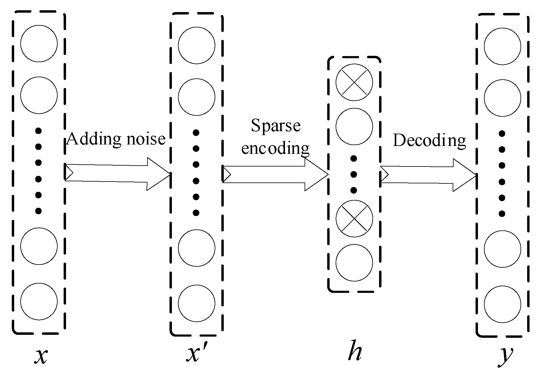
3.1. Feature Selection Based on Stacked Denoising Sparse Autoencoder

To depict the frequent pattern of FWH, it is necessary to determine the performance monitoring parameter in the first place. As mentioned in Section 2.2, the selection of performance monitoring parameter is not overly strict due to the greater concern about parameters’ relationship instead of accurate calculation of a certain parameter. From the viewpoint of the whole unit, the output of FWH consists of two parts: outlet feedwater and outlet drain water. Since most of the exchanged heat is carried by feedwater, the outlet feedwater temperature (OFT) can represent the main heat transfer process. Therefore, the OFT is selected as the performance monitoring parameter to describe heat transfer state. The terminal temperature difference (TTD) is a function of OFT and inlet steam pressure, and it can also represent the heat transfer state of FWH. However, there exist some problems if it is selected as performance monitoring parameter. When TTD is chosen as the performance monitoring parameter, the frequent pattern model needs to additionally learn the characteristics of vapor, which is of a high order nonlinear relationship. This will increase the training difficulty invisibly and may lead to a worse fault early warning performance. Hence, it is not adopted in this paper.
The input features selection to characterize frequent pattern model appropriately is another critical issue. To separate the coupling relationship in a high-pressure heating system, #2 FWH is regarded as a control body and only its direct-related parameters are selected in this paper as shown in Table 1. The #1 FWH inlet steam pressure is also considered as an alternative input feature since it represents the inlet drain water mass flow from #1 FWH. The #2 FWH drain water pressure (#2 DWP) is absent for the reason that the corresponding sensor is not installed in the researched FWH in this paper. Nonetheless, the #2 FWH inlet steam pressure has almost the same value except for small pressure loss and sensor noise since it obtains the vast majority of information in #2 FWH DWP. Therefore, the absence of #2 DWP will not have a significant impact on the results of this research.
Due to the underlying correlation and potential nonlinearity between parameters, the Spearman correlation coefficient is used to preliminary prescreen the input features. The higher the Spearman correlation coefficient is, the stronger the correlation between relevant features. As shown in Figure 6, all the Spearman correlation coefficients between related parameters exceed 0.75. It can be regarded that all parameters in Table 1 have a strong correlation with the OFT and also they have a high correlation between each other.
The above correlation analysis quantifies the correlation between relevant parameters. In order to analyze the data characteristics more intuitively, the typical load variation interval, which is the same as Section 2.1, is selected to display the duplicate information contained in parameters. Figure 7 illustrates the change of OFT, #1 drain water temperature (#1 DWT), #2 inlet feedwater temperature (#2 IWT) and #2 drain water temperature (#2 DWT), respectively. Figure 8 shows #1 extracted steam pressure (#1 ESP) and #2 extracted steam pressure (#2 ESP). Figure 9 shows #2 extracted steam temperature (#2 EST). It can be clearly seen in these figures that the above parameters have the same change tendency whether they are under the stable load or variable load condition, which means these features contain similar information.
In traditional research, any relevant parameters can be used as input features for modeling. But from the perspective of information theory, if all the parameters are taken as the model input, though more information can be obtained, more noises are introduced simultaneously. Furthermore, if too many parameters are used as model input features, too much duplicate information will be introduced, which is called redundant information in this paper. A fair amount of redundant information will bring a negative impact on fault early warning performance and conceal the fault weak symptoms. Therefore, further study in rational feature selection is required. Driven by that, this paper proposes a stacked denoising sparse autoencoder method for self-adaptive feature reduction for FWH.
Autoencoder (AE) is a kind of artificial neural network used in semi-supervised and unsupervised learning. Its function is to make representation learning by taking input information as an objective [23,24]. In order to force AE to learn useful information, noises are added to the input data [25], and then the network is trained to recover the original data without noise. Meanwhile, a sparse penalty is added to the encoding layer [26], which makes the AE try to limit the active neurons in the encoding layer and replace the original data with the discovery features. For the strong coupling characteristics of FWH, it is necessary to extract essential features from numerous information for frequent pattern characterization, and avoid information loss during the feature extraction procedure. Therefore, denoising sparse autoencoder (DSAE) is introduced to realize self-adaptive feature reduction, discover essential features automatically from unlabeled data and give a more concise feature description than original data form. The diagram of DSAE network is shown in Figure 10 and the algorithm implementation process presents as follows.
Firstly, white noise is added to the original input x to form the corrupted data x . Then, the encoding and decoding processes in DSAE are shown as Equations (5) and (6):
h = f 1 ( x ) = s ( w 1 x + b 1 )
y = f 2 ( h ) = s ( w 2 h + b 2 )
wherein s denotes the sigmoid activation function, w 1 , b 1 and w 2 , b 2 denote the weight and bias in the encoding layer and decoding layer.
To ensure the sparsity of the encoding layer, relative entropy (also called Kullback-Leibler divergence) is adopted to add a sparsity penalty to the loss function, which is described as Equation (7):
K L ( ρ ρ i ) = ρ log ρ ρ i + ( 1 ρ ) log 1 ρ 1 ρ i
wherein ρ denotes the sparsity parameter, which specifies desired level of sparsity, ρ i denotes the average activation of hidden unit. The loss function in DSAE is defined as Equation (8):
J s p a r s e ( w , b ) = 1 N k = 1 N y ( k ) x ( k ) 2 + λ ( w 1 F 2 + w 2 F 2 ) + η j = 1 k K L ( ρ ρ i )
In Equation (8), the first part is the squared-error cost function, the second part is the regularization penalty term to avoid the over-fitting problem, and the third part is the sparse penalty term, where η denotes weight of the sparsity penalty term. The backpropagation algorithm is used to update the parameters to minimize J s p a r s e ( w , b ) as a function of w and b . Due to the strong coupling and high correlation of relevant parameters illustrated above, gradual feature reduction is adopted to achieve essential feature extraction in this paper. Thus, the stacked denoising sparse autoencoder (SDSAE), which is composed of multiple DSAE units and constructed as a neural network, is adopted to achieve self-adaptive feature reduction in this paper.
After feature reduction by SDSAE, it is necessary to depict the nonlinear properties among FWH parameters. This paper selects BPNN to achieve this goal due to its powerful nonlinear regression ability. Backpropagation neural network (BPNN) is a multi-layer feedforward neural network [27], and its diagram is shown in Figure 11. Because the activation function introduces nonlinear factors into neurons, BPNN is adopted to express nonlinear properties between SDSAE output and the performance monitoring parameter. Therefore, SDSAE and BPNN are combined to produce self-adaptive feature reduction and nonlinear properties characterization. The diagram of SDSAE-BP network is shown in Figure 12.
Based on the above introduction of DSAE, the establishing process of SDSAE-BP network are elaborated as follows:
  • First, train DSAE1 with the initial input x, and obtains weight, bias of hidden layer w11, b11 and the corresponding output h1;
  • Then, train DSAE2 with the input h1, and obtains weight, bias of hidden layer w21, b21;
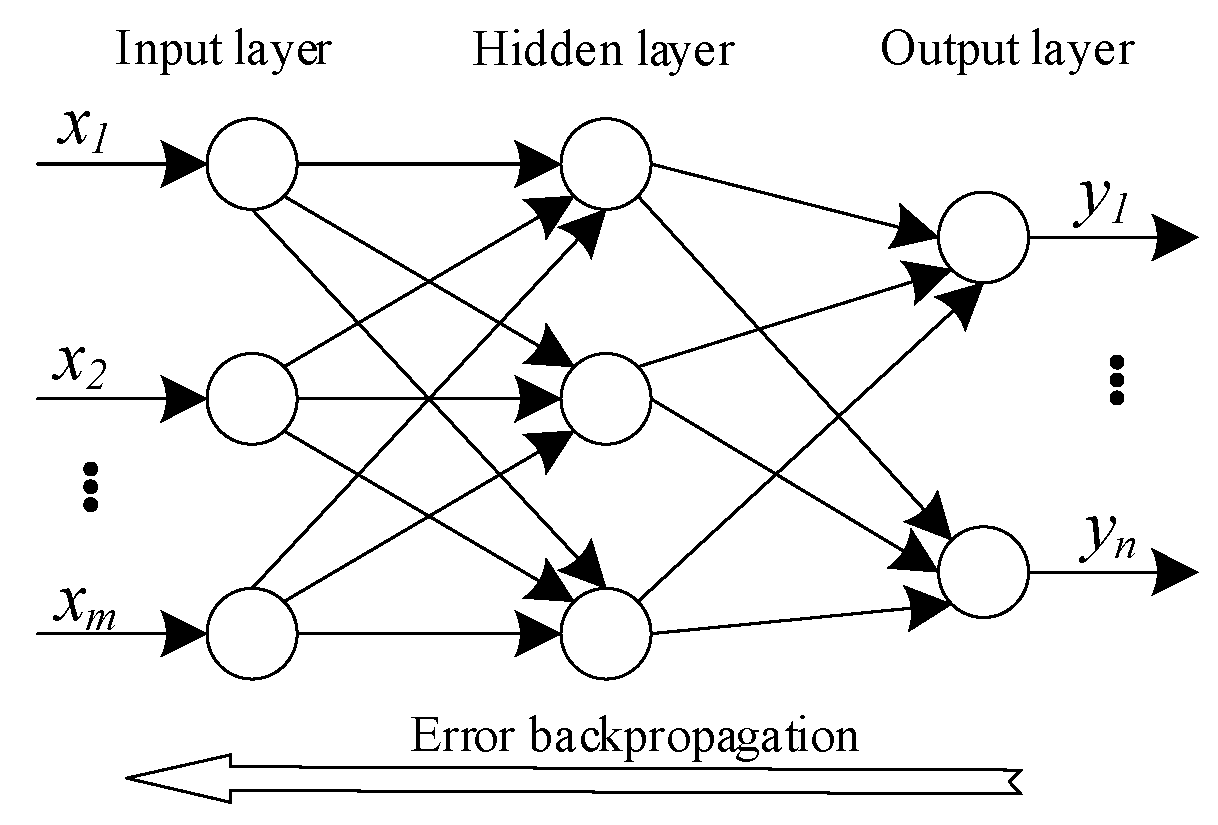
  • Finally, a three hidden layer neural network is constructed. The weight and bias of the first hidden layer and the second hidden layer are set to w11, b11 and w21, b21, and the parameters are not updated in the subsequent network training process. According to BP algorithm, the neural network parameters of the third hidden layer and output layer are trained.
Such an approach can realize the requirement of self-adaptive feature reduction and integrate SDSAE into the traditional BP neural network by pretraining the parameters of the first and second hidden layer neurons.

3.2. Technical Process of the Proposed Method

According to the definition of the frequent pattern model, the influence of working conditions should be fully considered when characterizing the frequent pattern. Theoretically, the residual between model output and measured value mainly comes from uncertain model error and noises which should also obey normal distribution. Thus, the Pauta criterion is adopted for fault early warning in this paper.
The standard deviation of the training set σ is obtained by analyzing the residuals of the training set. If the residuals are distributed in [ 3 σ , 3 σ ] , they are judged as normal data, otherwise, they are judged as fault data. To quantitatively evaluate the performance of fault early warning, this paper proposes the fault early warning accuracy as Equation (9), which refers to the definition of classification accuracy in classification issues:
A c c n o r m a l = n n o r N n o r , A c c a b n o r m a l = n a b n N a b n
wherein nnor is the number of residuals within the detection threshold in normal data, Nnor denotes the number of normal data, nabn is the number of residuals without detection threshold in fault data, Nabn denotes the number of fault data.
As mentioned above, technical process of the proposed method is shown as Figure 13.

4. Experiment

4.1. Data Preparation

As mentioned in Section 2.1, #2 high-pressure FWH of a typical 630 MW unit is selected as the research object. The data used in this study was collected from a distributed control system. According to the operation situation, the data is divided into two parts: the data during the period from 1 July 2017 to 21 July 2017 and the data during the period from 1 July 2018 to 21 July 2018. The practical unit was under maintenance during two periods. During the maintenance, it was found that there was obvious scaling, erosion marks and leakage points in #2 FWH. To improve FWH performance, the outer U-tube bundles were replaced, the inner tube bundles were chemically cleaned, and the leaking tubes were blocked in the maintenance process. Therefore, the maintenance makes an improvement in equipment performance.
After screening the start-up and shut-down data, there are 4,100,000 valid data left. As described in the technical process, the acquired data are divided into three sets, i.e., training set S 1 , validation set S 2 and fault early warning set S 3 . The data partition is shown in Figure 14. The data in S 1 and S 2 are all under normal conditions, whereas S 3 contained both normal and fault data to show the fault early warning performance. It must be noted that the data after maintenance, which is named as fault data, does not mean it is faulty but rather performance changing. The purpose of this data partition is to ensure that the frequent pattern model is trained under all working conditions.

4.2. Fault Early Warning Experiment

4.2.1. Frequent Pattern Modeling

In this section, the experiment is carried out to verify the performance of the proposed method in frequent pattern modeling. The training set is used for frequent pattern modeling and the validation set is used to adjust model hyperparameters as well as preliminarily verify the detection accuracy and robustness for normal data.
In this paper, root mean square error (RMSE) is used to quantify the model accuracy, and the index is defined as Equation (10):
RMSE = ( 1 N n = 1 N e 2 ) 1 2
wherein e denotes residual between model output and actual data, N denotes the number of data.
Tunable parameters in the SDSAE-BP network including the degradation rate, the number of hidden neurons, the number of epochs and other relative coefficients are obtained through a full factorial grid search with trial and error. The optimal hyperparameter combination is selected based on the minimum validation set residuals’ RMSE. The parameters involved in the SDSAE-BP network are set as shown in Table 2.
Figure 15 shows the verses of estimated value and actual data of performance monitoring parameter OFT in the training set, as well as corresponding residuals. As a result, the residuals have 0.0922 RMSE value and the residuals’ standard deviation σ is 0.0921. Correspondingly, the detection threshold is set to 0.2763 according to the Pauta criterion and represented by the two red lines in the figure. It can be found that the fact that the prediction error is low corresponds to the SDSAE-BP based frequent pattern model. Hence, it can be deemed that the trained model can describe frequent pattern in training set accurately.
Figure 16 and Figure 17 show the residuals and residuals’ distribution results in the validation set, respectively. The results illustrate that the distribution of the residuals approximates to a Gaussian distribution with zero means, which indicates that the model characterizes the internal relationship between input data and target data well, and proves the feasibility and effectiveness of the proposed method for FWH performance evaluation. Also, it elucidates that FWH performance remains unchanged in the validation set. Furthermore, the result confirms that the residuals caused by uncertain model error and noises are approximately normally distributed, thus the detection threshold determined by Pauta criterion is applicable in this study.

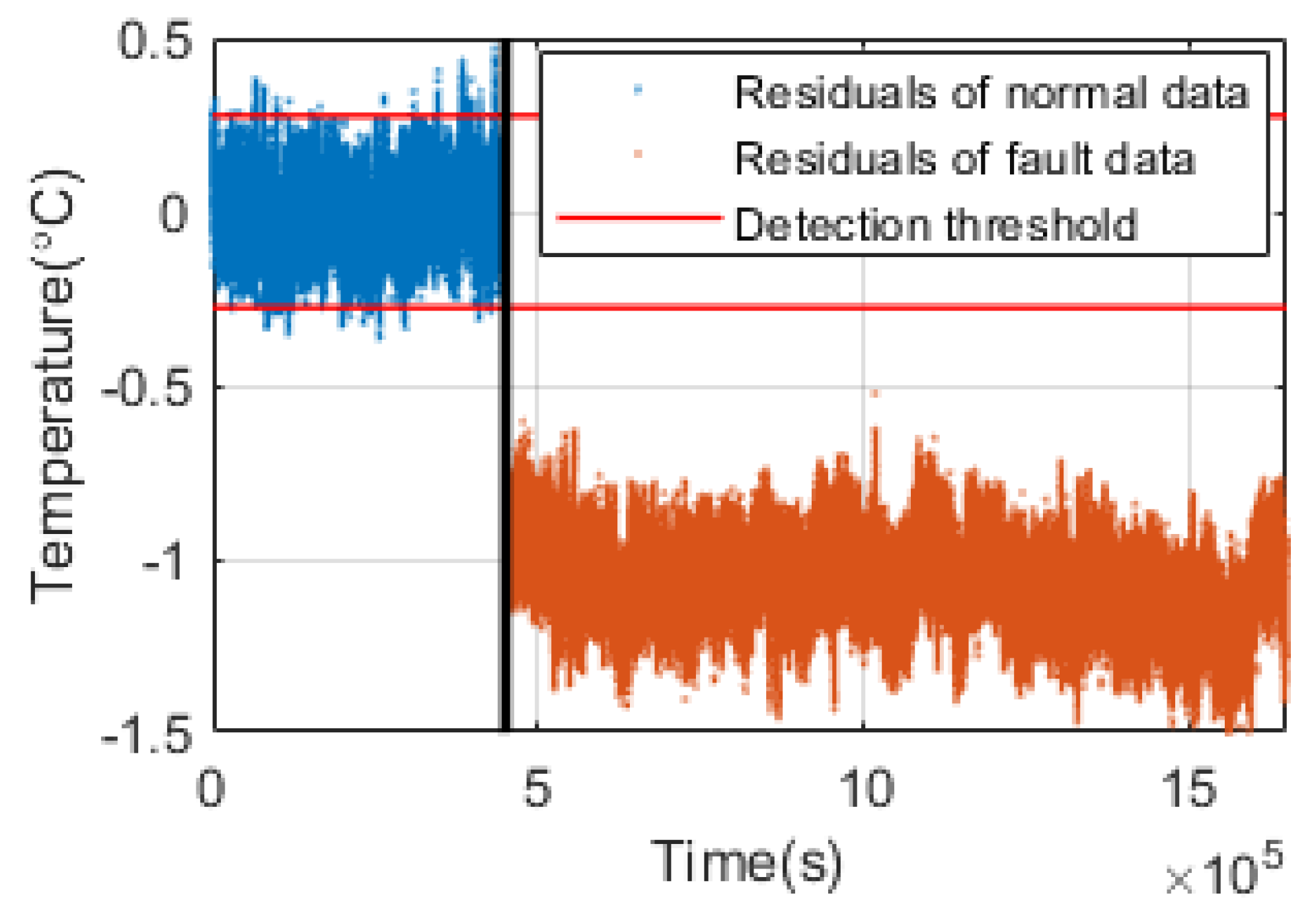
4.2.2. Fault Early Warning Experiment

To validate the fault early warning performance of the proposed method, the fault early warning set is used to verify its detection sensitivity and accuracy under various working conditions.
Figure 18 shows the predicted value versus actual data of OFT, and Figure 19 shows corresponding residuals in fault early warning set, wherein the red lines are the detection threshold [−0.2763, 0.2763] and the black line is the maintenance time. It can be seen that at the performance changing point, the residuals change significantly. From the results, 99.58% of normal data within the detection threshold, and 100% of the residuals of fault data exceed the detection threshold. The result proves that the FWH performance remains unchanged before maintenance and has an obvious performance change after maintenance. The negative residuals represent performance improvement. That is consistent with the actual operation state, and further proves that the proposed method is sensitive to fault and robust to various interferences.
For an intuitive description, the comprehensive performance of the SDSAE-BP-based frequent pattern model method is given in Table 3, wherein A c c n o r m a l and A c c f a u l t represent the accuracy of normal and fault data in fault early warning set, respectively.

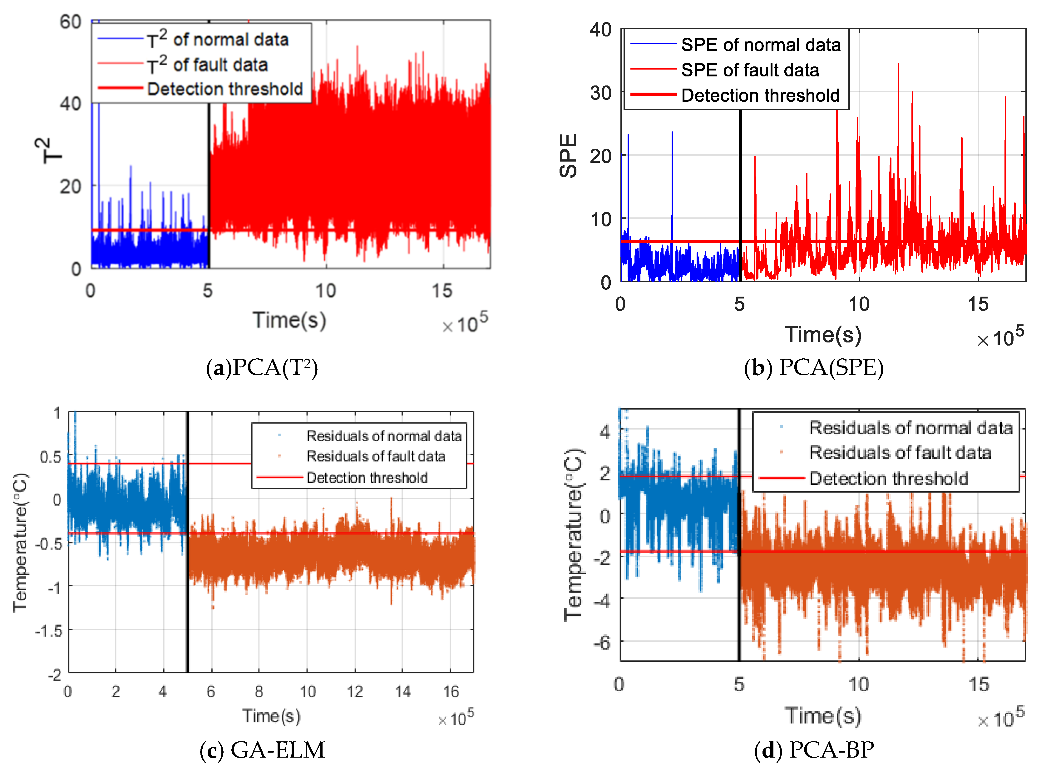
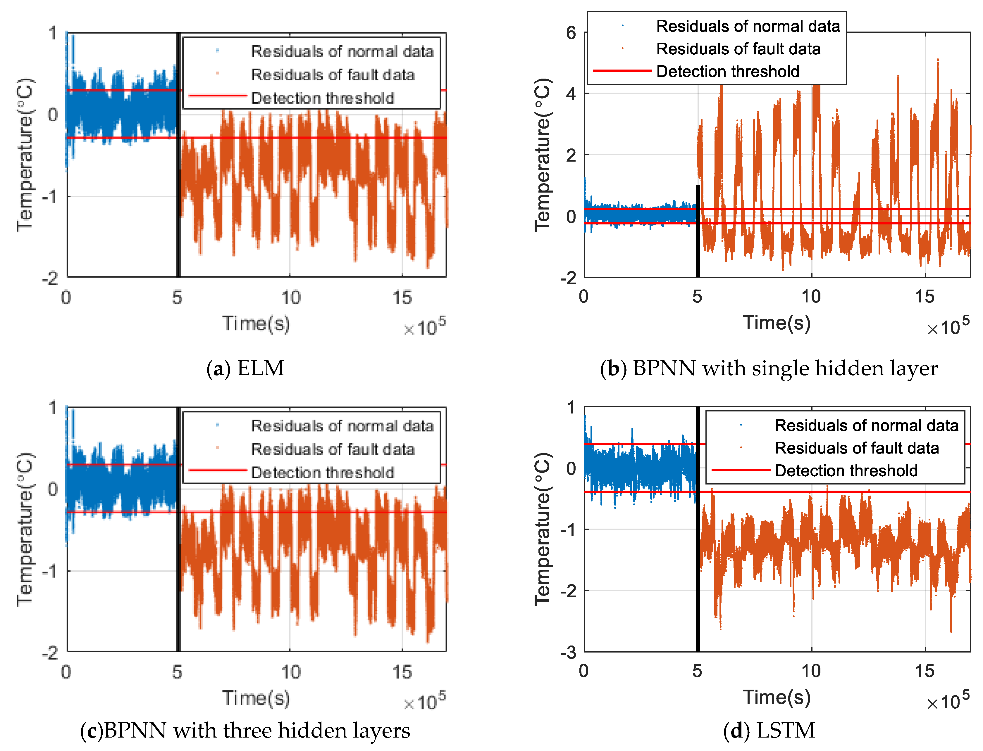
4.3. Comparison Experiment

In Section 3.1, an SDSAE-BP network is proposed for frequent pattern modeling to achieve self-adaptive feature reduction, which is the basis of consideration of redundant information caused by strong coupling of FWH and high correlation among relevant parameters. In subsequent sections, comparison experiments are carried out to further verify the necessity of feature reduction and the superiority of the SDSAE-based feature reduction method, separately.

4.3.1. The Necessity of Feature Reduction

To validate the necessity of feature reduction in FWH fault early warning, the comparative experiments are carried out for comparisons, which include: (1) Extreme learning machine (ELM) [28]; (2) BPNN with single hidden layer; (3) BPNN, whereas the hidden layer’s setting is same as that of proposed SDSAE-BP in Section 4.2.1; (4) Long short-term memory network (LSTM) [29]. Corresponding hyperparameters and hidden layer neuron numbers for the above methods are obtained through a full factorial grid search with trial and error. Considering the stochastic nature of the neural network in the training problem, each experiment is carried out 20 times and the one with minimum RMSE in the validation set is selected as the best result for comparison. The performance monitoring parameter and the data partition are exactly the same as utilized in the experiment with SDSAE-BP. The performance of comparative methods in fault early warning set are separately illustrated in Figure 20a–d, and the comprehensive comparison is shown in Table 4.
Comparatively speaking, the proposed SDSAE-BP based method achieves the best fault early warning performance. Although other methods may achieve good results in training set and obtain smaller detection threshold, the overall performance is poor in other data sets. Meanwhile, it is worth noticing that the residuals present the same fluctuation trend with the unit load as shown in all comparison methods, which illustrates the adverse impact of redundant information on fault early warning.
In the experiment, BPNN with a single hidden layer is directly used to do frequent pattern modeling. From results, although it has a good fitting result in training set and the detection threshold is smaller than 5, the fault early warning performance in S 3 is poor. The introduction of redundant information leads to a decrease in the sensitivity of the fault data, which will finally lead to the decline of the fault early warning performance. Furthermore, 3 experiment, wherein BPNN with the same hidden layer neurons setting of the proposed 5 method, is conducted as a comparative experiment. The purpose of the setting is to verify the superiority of the network parameters pretrain carried out by SDSAE. In principle, the parameter setting of hidden layer neurons (7–4–7) can approximately realize the feature compression for the first, and the second hidden layer transmits fewer features to the next layer. However, although the structure of the proposed SDSAE-BP is imitated, the pretrain process of network parameters is absent in the comparative 5 experiment. Thus, the proposed SDSAE-BP method obtains better performance than the 5 since the SDSAE fulfills the feature reduction and obtains a more essential feature expression for frequent pattern modeling. Meanwhile, although 5 does not achieve the best feature reduction effect, it is better than 2 with no thought for feature reduction.
For 4, the performance of the LSTM network is better than 1 to 3. Compared with traditional neural networks, LSTM-based deep learning methods have more powerful cognitive capability in feature learning, which can discover the data characteristics and reduce the negative impact of redundant information to some extent. As can be seen, the LSTM-based method has less residual fluctuation compared with 1 and 3. The proposed SDSAE-BP-based method outperforms LSTM in both detecting threshold and discriminating degree of fault symptoms. Although the detection accuracy of No.4 has little difference with No.5, the proposed SDSAE-BP method outperforms the sensitivity of fault characteristics.
In addition, it can be seen that BPNN outperforms ELM. This is because the weight and bias of the ELM hidden layer is given randomly, and it cannot be updated when network parameters are modified. The updating of network parameters is beneficial to frequent pattern modeling.

4.3.2. Superiority of SDSAE based Feature Reduction Method

For the proposed method, SDSAE is used to realize self-adaptive feature reduction and extract the essential features from redundant information. However, there are many feature reduction methods used in similar previous researches. In this section, comparative experiments are conducted with models using different feature reduction methods. The comparative experiments include: (1) Squared prediction error (SPE) based principle component analysis (PCA) fault diagnosis method; (2) T2 based PCA fault diagnosis method; (3) Genetic algorithm based ELM (GA-ELM) method, which selects input features with the goal of minimizing RMSE value of validation set; (4) BPNN based on PCA feature reduction, where the cumulative variance contribute rate is set to 0.99. The performance monitoring parameter and data partition are the same as the experiment in Section 4.2. Figure 21a–d shows the performance of each method separately, and Table 5 shows the comparison results with different feature reduction methods.
As can be seen in Table 5, the proposed SDSAE-BP-based method achieves the best performance. Compared with other methods, the conclusions can be drawn as follows.
Firstly, the SPE- and T2-based PCA fault diagnosis methods achieve fault early warning by analyzing the data statistical properties. However, the above methods only consider the statistical characteristics of data. The proposed frequent pattern model-based method not only considers the data characteristics, but also integrates the physical mechanism of FWH closely. Thus, the proposed method achieves a more desirable overall performance.
Secondly, the result of GA-based feature reduction experiment 4 is taking #2 FWH inlet feedwater temperature and #2 FWH inlet steam pressure as model input features. From the perspective of FWH working principles, it is reasonably explained that the above two parameters represent the main driving force of parameters changing. However, it is generally known that feature reduction will lead to information loss. Although the GA-based feature selection method avoids the problem carried by redundant information, it also discards the effective information contained in unselected parameters. SDSAE can reduce the interferences of redundant information while retaining more effective information through self-adaptive feature reduction and nonlinear transformation; thus, it achieves better performance than the GA-ELM method.
Finally, although the SDSAE has similarity with PCA in feature reduction, it is much more flexible since it can represent both linear and nonlinear transformation, while PCA can only perform linear. Meanwhile, the SDSAE can learn more essential data characteristics than PCA-based methods by setting appropriate noise and sparse constraints. In practical application, the information contained in the SDSAE significantly improves the frequent pattern characterization ability and obtains better performance than the PCA-BP method.

5. Conclusions

In this paper, a fault early warning method based on SDSAE-BP frequent pattern model for feedwater heater performance degradation is developed. Firstly, the concept of a frequent pattern model is proposed as an indicator for FWH performance evaluation, which avoids the influence of working conditions. Then, considering the negative effects carried by redundant information, the SDSAE and BPNN are combined to achieve self-adaptive feature reduction and nonlinear properties characterization for frequent pattern modeling. Through the experiment with actual data collected from a typical FWH, the results show that the proposed method achieves 99.58% and 100% for normal and fault data, respectively. Moreover, comparative experiments are carried out to verify the necessity of feature reduction as well as the rational balance between effective information and interferences. The SDSAE-based feature reduction method outperforms traditional methods in essential feature extraction and effective information retention.
The method proposed in this paper not only provides a new approach for the fault early warning of FWH performance degradation, but also provides the basic technology for study on subsequent failure trend prediction and condition-based maintenance combined with time-series analysis. The related research achievements have significant meanings in theory and practical engineering.

Author Contributions

X.L. (Xingshuo Li): Conceptualization, Methodology, Validation, Writing—original draft preparation. J.L. (Jiajia Li): Writing—review & editing. J.L. (Jinfu Liu), Investigation, Data curation. X.L. (Xianling Li): Resources. P.Y.: Data curation. D.Y.: Supervision. All authors have read and agreed to the published version of the manuscript.

Funding

This work was supported by National Key R&D Program of China No. 2017YFB0902100, Science and Technology on Thermal Energy and Power Laboratory Foundation No.TPL2017CA010, National Natural Science Foundation of China No.51976042 and the National Science and Technology Major Project of China No. 2017-I-0007-0008.

Acknowledgments

The authors would like to thank the anonymous reviewers for their valuable suggestions to refine this work.

Conflicts of Interest

The authors declare that they have no conflict of interests.

References

  1. Baldwin, T.; Tawfik, M.; Bond, L. Report from the Light Water Reactor Sustainability Workshop on On-Line Monitoring Technologies; Technical Report No. INL/EXT-10-19500; Idaho National Laboratory (INL): Idaho Falls, ID, USA, 2010.
  2. Series, I.N.E. On-line Monitoring for Improving Performance of Nuclear Power Plants Part 2: Process and Component Condition Monitoring and Diagnostics; International Atomic Energy Agency (IAEA): Vienna, Austria, 2008. [Google Scholar]
  3. Akhtar, S.Z.; Phipps, M. Considerations for safe and effective design of feedwater heaters. Hydrocarb. Process. 2008, 87, 71–75. [Google Scholar]
  4. Vandani, A.M.K.; Joda, F.; Ahmadi, F.; Ahmadi, M.H. Exergoeconomic effect of adding a new feedwater heater to a steam power plant. Mech. Ind. 2017, 18, 224. [Google Scholar]
  5. Riesgo, A.; Folgueras, M.B. One feedwater heater taken out of service as a strategy to maintain full load and its effect on steam power cycle parameters and performance. Int. J. Energy Res. 2019, 43, 2296–2311. [Google Scholar]
  6. Zangeneh, S.; Bakhtiari, R. Failure investigation of a deaerating feed-water heater in a power plant. Eng. Fail. Anal. 2019, 101, 145–156. [Google Scholar]
  7. Karg, D.C.; Henderson, T.N.; Svensen, L.M., III. Analysis of feedwater heater performance data to detect and monitor pass partition plate leakage. In Proceedings of the 1996 International Joint Power Generation Conference, American Society of Mechanical Engineers, New York, NY, USA, 13–17 October 1996. [Google Scholar]
  8. Shabani, G.A.S.; Ameri, M.; Akbari, O.; Seifi, A. Performance assessment and leakage analysis of feed water pre-heaters in natural gas–fired steam power plants. J. Power Technol. 2018, 98, 352–364. [Google Scholar]
  9. Barszcz, T.; Czop, P. Estimation of feedwater heater parameters based on a grey-box approach. International J. Appl. Math. Comput. Sci. 2011, 21, 703–715. [Google Scholar]
  10. Barszcz, T.; Czop, P. A feedwater heater model intended for model-based diagnostics of power plant installations. Appl. Therm. Eng. 2011, 31, 1357–1367. [Google Scholar]
  11. Zhao, Y.; Wang, C.; Liu, M.; Chong, D.; Yan, J. Improving operational flexibility by regulating extraction steam of high-pressure heaters on a 660 MW supercritical coal-fired power plant: A dynamic simulation. Appl. Energy 2018, 212, 1295–1309. [Google Scholar]
  12. Chen, C.; Zhong, X.; Xiao, J.; Zhu, Y.; Jiang, J. Performance monitoring of regenerative system based on dominant factor method. In Proceedings of the ASME 2017 Power Conference Joint With ICOPE-17 collocated with the ASME 2017 11th International Conference on Energy Sustainability, the ASME 2017 15th International Conference on Fuel Cell Science, Engineering and Technology, and the ASME 2017 Nuclear Forum, Charlotte, NC, USA, 26–30 June 2017; American Society of Mechanical Engineers Digital Collection, 2017. [Google Scholar]
  13. Jiang, X.; Liu, P.; Li, Z. A data reconciliation based approach to accuracy enhancement of operational data in power plants. Chem. Eng. 2013, 35, 1213–1218. [Google Scholar]
  14. Wang, X.; Ma, L.; Wang, T. An optimized nearest prototype classifier for power plant fault diagnosis using hybrid particle swarm optimization algorithm. Int. J. Electr. Power Energy Syst. 2014, 58, 257–265. [Google Scholar]
  15. Li, F.; Upadhyaya, B.R.; Coffey, L.A. Model-based monitoring and fault diagnosis of fossil power plant process units using group method of data handling. ISA Trans. 2009, 48, 213–219. [Google Scholar] [PubMed]
  16. Kang, Y.K.; Kim, H.; Heo, G.; Song, S.Y. Diagnosis of feedwater heater performance degradation using fuzzy inference system. Expert Syst. With Appl. 2017, 69, 239–246. [Google Scholar]
  17. Ma, L.; Ma, Y.; Lee, K.Y. An intelligent power plant fault diagnostics for varying degree of severity and loading conditions. IEEE Trans. Energy Convers. 2010, 25, 546–554. [Google Scholar]
  18. Ma, L.; Wang, X.; Cao, X. Feedwater heater system fault diagnosis during dynamic transient process based on two-stage neural networks. In Proceedings of the 32nd IEEE Chinese Control Conference, Xi’an, China, 26–28 July 2013; pp. 6148–6153. [Google Scholar]
  19. Ma, L.; Ma, Y.; Ma, J. Fault diagnosis for the feedwater heater system of a 300mw coal-fired power generating unit based on RBF neural network. In Advances in Machine Learning and Cybernetics; Springer: Berlin/Heidelberg, Germany, 2006; pp. 832–841. [Google Scholar]
  20. Heo, G.; Lee, S.K. Internal leakage detection for feedwater heaters in power plants using neural networks. Expert Syst. Appl. 2012, 39, 5078–5086. [Google Scholar]
  21. Garcia, R.F. Improving heat exchanger supervision using neural networks and rule based techniques. Expert Syst. Appl. 2012, 39, 3012–3021. [Google Scholar]
  22. Radhakrishnan, V.R.; Ramasamy, M.; Zabiri, H.; Do Thanh, V.; Tahir, N.M.; Mukhtar, H.; Hamdi, M.R.; Ramli, N. Heat exchanger fouling model and preventive maintenance scheduling tool. Appl. Therm. Eng. 2007, 27, 2791–2802. [Google Scholar]
  23. Bengio, Y.; Courville, A.; Vincent, P. Representation learning: A review and new perspectives. IEEE Trans. Pattern Anal. Mach. Intell. 2013, 35, 1798–1828. [Google Scholar] [PubMed]
  24. Goodfellow, I.; Bengio, Y.; Courville, A. Deep Learning; Cambridge MIT Press: Cambridge, MA, USA, 2016; Chapter 14; Volume 1, pp. 499–507. [Google Scholar]
  25. Vincent, P.; Larochelle, H.; Bengio, Y.; Manzagol, P.A. Extracting and composing robust features with denoising autoencoders. In Proceedings of the International Conference on Machine Learning, Helsinki, Finland, 5–9 June 2008; pp. 1096–1103. [Google Scholar]
  26. Xu, J.; Xiang, L.; Liu, Q.; Gilmore, H.; Wu, J.; Tang, J.; Madabhushi, A. Stacked Sparse Autoencoder (SSAE) for Nuclei Detection on Breast Cancer Histopathology Images. IEEE Trans. Med Imaging 2016, 35, 119–130. [Google Scholar] [PubMed] [Green Version]
  27. Hecht-Nielsen, R. Theory of the backpropagation neural network. In Neural Networks for Perception; Academic Press: Cambridge, MA, USA, 1992; pp. 65–93. [Google Scholar]
  28. Huang, G.B.; Zhu, Q.Y.; Siew, C.K. Extreme learning machine: Theory and applications. Neurocomputing 2006, 70, 489–501. [Google Scholar]
  29. Hochreiter, S.; Schmidhuber, J. Long short-term memory. Neural Comput. 1997, 9, 1–32. [Google Scholar]
Figure 1. Structure of FWH.
Energies 13 06061 g001
Figure 2. Thermodynamic diagram of #2 FWH.
Energies 13 06061 g002
Figure 3. Unit load and corresponding k and TTD.
Energies 13 06061 g003
Figure 4. Schematic diagram of fault influence mechanism.
Energies 13 06061 g004
Figure 5. Diagram of proposed frequent pattern model-based method.
Energies 13 06061 g005
Figure 6. Spearman correlation coefficient map for preliminary selected parameters.
Energies 13 06061 g006
Figure 7. The water temperature duration curve.
Energies 13 06061 g007
Figure 8. The pressure duration curve.
Energies 13 06061 g008
Figure 9. The #2 EST temperature duration curve.
Energies 13 06061 g009
Figure 10. Diagram of DSAE network.
Energies 13 06061 g010
Figure 11. Diagram of BPNN.
Energies 13 06061 g011
Figure 12. Diagram of SDSAE-BP network.
Energies 13 06061 g012
Figure 13. Technical process of the proposed fault early warning method.
Energies 13 06061 g013
Figure 14. Data partition.
Energies 13 06061 g014
Figure 15. Fitting result in training set.
Energies 13 06061 g015
Figure 16. Residuals in validation set.
Energies 13 06061 g016
Figure 17. Residual distribution in validation set.
Energies 13 06061 g017
Figure 18. Performance in fault early warning set.
Energies 13 06061 g018
Figure 19. Corresponding residuals in fault early warning set.
Energies 13 06061 g019
Figure 20. Fault early warning performance of comparative methods.
Energies 13 06061 g020
Figure 21. Fault early warning performance of comparative feature reduction methods.
Energies 13 06061 g021
Table 1. Preliminary selection features for modeling
No.ParameterNo.Parameter
1#2 FWH inlet feedwater temperature7#2 FWH drain water temperature
2#2 FWH U-tube metal temperature8#2 FWH water level
3Feedwater mass flow9#2 FWH extraction steam pressure
4Feedwater pressure10#2 FWH extraction steam temperature
5#1 FWH extraction steam pressure11OFT
6#1 FWH drain water temperature
Table 2. Parameters setting of SDSAE-BP network
HyperparametersDSAE1DSAE2BPNN
Degradation rate0.10.1-
Hidden layer neurons747
Epochs1000500500
L2 Regularization coefficient0.0010.001-
Sparse regularization coefficient44-
Sparse parameter0.050.05-
Decoder transfer functionPurelinPurelin-
Table 3. Overall fault early warning performance of the proposed method
Training RMSEValidation RMSEDetection ThresholdAccuracy of Training SetAccuracy of Validation SetFault Early Warning Set
AccnormalAccfault
0.09220.10060.27630.99670.98630.99581.0000
Table 4. Performance comparison of different modeling methods.
No.Modeling MethodHidden Layer NeuronsDetection ThresholdAccuracy of Training SetAccuracy of Validation SetFault Early Warning Set
AccnormalAccfault
1ELM(35)0.35120.99250.91510.89580.9316
2BPNN(30)0.23490.99490.91900.95130.9267
3BPNN(7-4-7)0.24620.99450.91170.95370.9716
4LSTM(30)0.39080.99580.99240.99570.9927
5SDSAE-BP(7-4-7)0.27630.99670.98630.99581.0000
The bold is to show the best performance in the comparative test.
Table 5. Performance comparison of feature reduction methods.
No.Modeling MethodDetection ThresholdAccuracy of Training SetAccuracy of Validation SetFault Early Warning Set
AccnormalAccfault
1PCA(T2)9.21040.99580.98200.99250.9506
2PCA(SPE)6.27630.97770.94920.98830.3097
3GA-ELM0.39810.99110.98330.98600.9888
4PCA-BP1.76580.98690.95760.98560.9248
5SDSAE-BP0.27630.99670.98630.99581.0000
The bold is to show the best performance in the comparative test.
Publisher’s Note: MDPI stays neutral with regard to jurisdictional claims in published maps and institutional affiliations.

