Comparison of New Anomaly Detection Technique for Wind Turbine Condition Monitoring Using Gearbox SCADA Data

Abstract

Anomaly detection for wind turbine condition monitoring is an active area of research within the wind energy operations and maintenance (O & M) community. In this paper three models were compared for multi-megawatt operational wind turbine SCADA data. The models used for comparison were One-Class Support Vector Machine (OCSVM), Isolation Forest (IF), and Elliptical Envelope (EE). Each of these were compared for the same fault, and tested under various different data configurations. IF and EE have not previously been used for fault detection for wind turbines, and OCSVM has not been used for SCADA data. This paper presents a novel method of condition monitoring that only requires two months of data per turbine. These months were separated by a year, the first being healthy and the second unhealthy. The number of anomalies is compared, with a greater number in the unhealthy month being considered correct. It was found that for accuracy IF and OCSVM had similar performances in both training regimes presented. OCSVM performed better for generic training, and IF performed better for specific training. Overall, IF and OCSVM had an average accuracy of 82% for all configurations considered, compared to 77% for EE.

1. Introduction

Wind turbines now generate a large proportion of the UK electricity demand. Operations and maintenance (O & M) has become a more significant area in the wind industry, especially in terms of cost of energy. The National Renewable Energy Laboratory has stated that operational expenditure (OPEX) costs for U.S. offshore wind energy is around £62-187/kW/year [1], this can be as much as 25 to 30% of the cost of a wind farm itself [2]. Such costs can be quite prohibitive for offshore wind. Offshore wind farms on average have a failure rate of 10 failures per turbine per year, with 17.5% being major repairs, and 2.5% being major replacements [3].

One of the components that is most problematic for wind turbines is the gearbox. The gearbox itself causes 0.6 days of downtime per year on average according to [4] with 6.21 days of downtime per failure on average. One paper [3] has stated that the gearbox failed roughly 0.6 times per year per turbine, with just over 24% of these being a major replacement of the gearbox. When compared to the previous values stated for the turbine overall, the gearbox requires replacement more regularly. Offshore major replacements can lead to even longer downtimes when accounting for weather windows and availability of vessels.

One technique that has been suggested to reduce the amount of unplanned downtime is condition based maintenance. Such an approach to maintenance requires monitoring the component condition. Maintenance action is then carried out based on the health of the component [5]. The other methods of maintenance being corrective and scheduled maintenance. Corrective maintenance is only performed when a failure occurs, with no ability to plan around weather and component availability. Scheduled maintenance is used currently in offshore wind, and this is when maintenance is done during scheduled visits to the turbine, with corrective maintenance being carried out when required. Scheduled maintenance then does allow some planning around the factors discussed previously. By analysing faults with condition monitoring component faults can be predicted or diagnosed, and one of the most effective methods at this is anomaly detection.

Anomaly detection has been of recent interest to researchers within wind energy as a means to diagnose or predict faults within one, or multiple components of the turbine. This typically involves using data features to determine the normal behaviour of the turbine, which can then be used as a threshold or guide to assess if new data is anomalous.

This paper compares different Anomaly Detection models for use on Supervisory Control and Data Aquisition (SCADA) data from operational wind turbines. Three different anomaly detection techniques will be compared based on their performance at identifying healthy and unhealthy behaviour of wind turbine gearboxes. The authors present a novel method of Anomaly Detection that utilises less data, only requiring two months of data at a time. The method currently compares data one year apart, by investigating the difference in anomaly count between months, anomalies are defined later in Section 3.4. Two different training regimes (Section 3.1) are investigated, with a comparison being made for both to assess which is more appropriate.

The use of only two months of data was a request from the industrial partner to investigate whether there is a requirement to store and analyse long term data, or if it were possible to perform health classification using less data. The advantages of this would be the shorter run time for training and testing, and also less storage being required to keep the data over such long periods for immediate access and analysis. This approach is a comparative assessment of the performance of several models using such restricted data, to find if the turbines are operating in a healthy condition or not. Whilst computational time, and storage, are not major factors for the quantity of data used in this paper, the industrial partner is interested due to their management of fleets of turbines. The computational times presented in this paper would then become a greater factor when looking at many thousands of turbines.

Based on the authors’ literature review, the contributions of this paper are:

• The use of only two months of data for turbine health classification.
• Isolation Forest and Elliptical Envelope have not previously been used for wind turbine fault detection.
• One Class Support Vector Machine has not been used for wind turbine SCADA fault detection
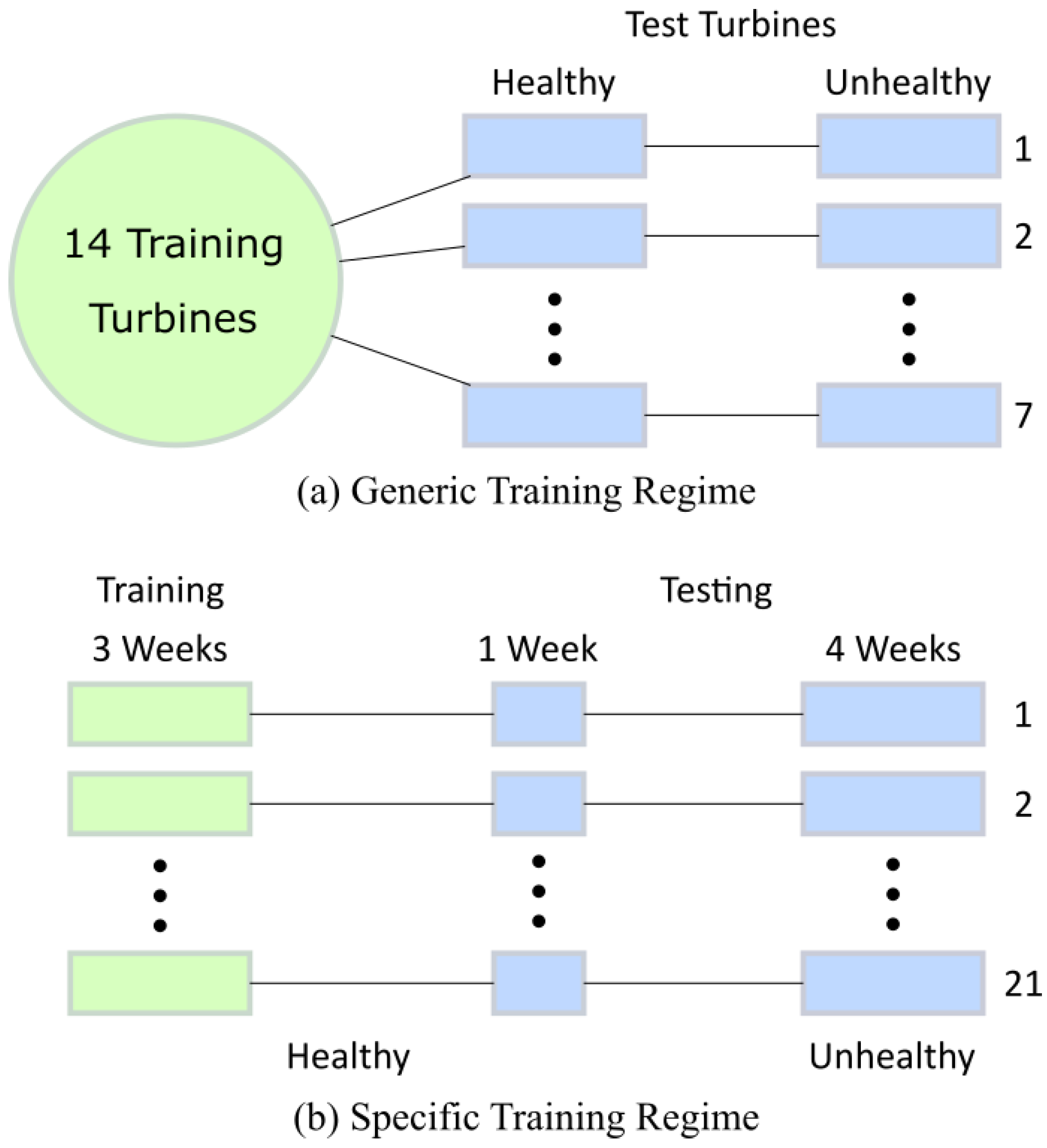
• Comparing training techniques, generic and specific, for wind turbines.

The structure of the paper is as follows. Section 2 is a literature review for the three models used in this paper and how they’ve been used previously. Section 3 explores the methodology used in this paper, including a description of the data used and the test descriptions. Section 4 shows the accuracy for each different model for the different data configurations, with some discussion to elaborate on the results.

2. Literature Review

This section presents previous work in the field of condition based maintenance for wind turbines. Typically these techniques utilise either vibration data from bespoke condition monitoring systems (CMS), or features from SCADA systems.

Some recent examples of fault detection for vibration data from wind turbines are presented here. Purarjomandlangrudi et al. [6] presented a technique that extracts Gaussian parameters from vibration data for wind turbines bearing faults, and compared this to OCSVM. It was shown to be able to predict its first anomaly 100 hours before failure, and 25 hours before OCSVM. Xu et al. [7] uses Local Outlier Factor (LOF) to detect abnormal segments within vibration samples from a wind turbine. Principal components were extracted from time domain features, and then fed into the LOF to determine abnormality. It was found that the k nearest neighbours in LOF was an important parameter for this technique. Ogata et al. [8] presented a technique using Gaussian Mixture Models (GMMs) trained on Fourier local auto-correlation and other time domain features of vibration data for a wind turbine low speed bearing. The anomaly score could be seen to strongly trend upwards before failure. Abouel-seoud [9] examined time domain features for vibration data measured from a test rig gearbox. This test rig had faults introducted artificially to it, and one second measurements were taken six times over 7 h. The trend of the time domain features was examined and it was found the root mean square (RMS) of the signal showed a trend upwards towards failure for all cases considered. Huitao et al. [10] presented a technique utilising a wavelet neural network for a test rig gearbox. The network outputs a range of probabilities that the input data corresponds to a specific fault out of five possibilities, and was shown to perform better than Empirical Model Decomposition (EMD). Yu et al. [11] tested a Deep Belief Network, made up of stacked Restricted Boltzmann Machines trained unsupervised, on a benchmark 4.8 MW simulink wind turbine model. The model was investigated for different sensor, actuator, and system faults, and compared against multiple model and data driven techniques. It was found, based on all metrics examined, to perform better than the others.

SCADA data has also been examined for wind turbine condition monitoring. Zhao et al. [12] utilised a Deep Auto-Encoder to reconstruct SCADA variables for three different turbine faults. The errors of the reconstructed features were compared to a threshold developed with extreme value theory and was found to detect failure up to 10 hours quicker than a conventional neural network model, and had a comparable computational time. Rezamand et al. [13] presented a technique using a wavelet probability distribution function (PDF) to detect incipient fault, with a regressional neural network used for data imputation. Recursive Principal Component Analysis (PCA) was used to extract features, and the Debauchie wavelet was used to extract the PDF, which was shown to decline close to failure. If this crossed a threshold then failure was detected. Qu et al. [14] presented a technique that utilised a combination of linguistic terms and errors produced by a neural network to produce fault factors, which could predict failure and their severity. Pei et al. [15] presents a technique that uses K Nearest Neighbours (knn) to detect incipient failure in two turbines up to 6 months before failure. An instability factor, which was the sequential difference in distances for each new k, was compared to a threshold to detect the upcoming failure. Sun et al. [16] presented a technique for anomaly detection using a Stacked Denoised Auto-Encoder (SDAE) to extract features and feed this into a Clustering in Quest (CLIQUE) model. This method could classify the outlier with unsupervised learning, however knowledge of the outliers were known in advance for validation. Overall, this technique had a 98% classification accuracy, which was comparable to other models. Yan et al. [17] uses two back propagated Neural Networks (BPNNs), one to select relevant features, and the other to detect anomalies based on the RMSE between the real and predicted target for a 1.5 MW wind turbine. This model was able to predict failure 15 days in advance. Zhao et al. [18] presented a technique to both detect anomalies and predict remaining useful life. Density-Based Spatial Clustering of Applications with Noise (DBSCAN) was used to generate an anomaly proportion in the data, and a Support Vector Machine (SVM) was used to classify these as anomalous or not. An auto-regressive integrated moving average (ARIMA) model was then used to analyse the future performance of the wind turbine and to generate the remaining useful life, and this was done with only a mean relative error of 0.27 and could detect faults ahead of time by 44 days. This technique appears closest to the health classification method presented here, however it is applied to long term continuous data. Two papers [19,20] present the use of nonlinear auto-regressive neural networks with exogenous inputs (NARXs) for anomaly detection. The NARX models were used to predict some target feature, and then the Mahalanobis distance for each data pair of the error and actual target value was found. A threshold was developed to then determine what was anomalous, and if this was crossed continuously then an alarm was generated. This was successful, however it does require longer term data than provided for this paper. A third paper [21] utilised the same technique, however the Mahalanobis distances were denoised using a wavelet transform. For both faults considered, this provided a marked improvement over the raw Mahalanobis distance—increasing fault detection time by months.

2.1. Previous Examples of the Models Examined in this Paper

Various outlier detection models were considered for the paper, but this was narrowed down to three. Logistic regression was considered, however this requires supervised learning. As the labels for the data are not previously known, logistic regression was no longer an option. Another model considered was local outlier factor (LOF). This is an unsupervised learning model but cannot be trained and saved for repeated use. This technique would therefore be unsuitable for the generic training regime presented in this paper.

The three models used in this paper are commonly used for outlier detection. For the most part this has been within the realm of computer networks, with little application to wind energy. One Class Support Vector Machines facilitate a boundary around the normal data during training, this boundary is then used on to identify outliers, as shown in Figure 1a). Isolation Forest is made up of multiple Decision Trees, which averages the results of the ensemble of Decision Trees. The Isolation Forest defines an anomaly by a number of questions that distinguish it from the other data, this is shown in Figure 1b). Isolation Forest is a random forest of Decision Trees that identify anomalies through taking the average number of partitions required to isolate each individual data point. The data points with the fewest partitions are then identified as outliers. For example a sparse data-point would only require fewer partitions to distinguish it from all other data, compared to a data-point in a denser cluster. Finally, Elliptical Envelope which tries to fit an ellipse around the data using minimum covariance determinant (in blue), compared to an ellipse created by Mahalanobis distance (in red), as illustrated in Figure 1c).

The first model examined in this paper is One Class Support Vector Machines (OCSVMs). This model is a version of Support Vector Machine (SVM) that produces a hyperplane around the training data, which is then used to decide on whether future data is similar to this class, or is an anomaly. This model recognises the normal behaviour and then decides on whether the future data is also normal.

OCSVM uses what are known as support vectors to decide on the boundary. These support vectors are just data-points that are close to the boundary of the data. In a conventional SVM this would be the boundary between two or more classes. As OCSVM is a boundary based method, it means that outliers in the training data can degrade the performance of the model [23]. OCSVM separates the data by trying to solve the following equation: [24]

$$\underset{w\in F,ϵ\in R^l,\rho \in R}{min}\frac{1}{2}{\parallel w\parallel }^2+\frac{1}{{\nu }^l}\sum _i{ϵ}_i-\rho ,$$

(1)

subject to $(w\ast \Phi \left(x_i\right))\ge \rho -{ϵ}_i,{ϵ}_i\ge 0$. Where w is the weights of the function, $ϵ$ are the slack variables in the margin to produce a soft margin that will help prevent overfitting, $\rho$ is an offset parameterising a hyperplane in the feature space associated with the kernel, $x_i$ are the input values, and $\mathsf{\Phi }\left(x_i\right)$ maps these inputs from input space to feature space allowing for a hyperplane splitting the data classes to be formed. This hyperplane translates to a boundary around the data in the input space. In Equation (1) non-zero ${ϵ}_i$ are penalised, meaning that the decision function, presented by Scholkopf et al.: [24]

$$f\left(x\right)=sign((w\ast \mathsf{\Phi }\left(x_i\right))-\rho ),$$

(2)

should be positive for most input examples, i.e., they will be considered normal, while the regularisation term ($\parallel w\parallel$) shown in Equation (1), should remain small. This is determined by the variable ${\nu }^l$, which is the contamination hyperparameter discussed later in Section 3.3. This model should then output a positive 1 for most data in the centre, meaning normal, and a negative 1 for data elsewhere, meaning abnormal.

OCSVM has been used for some applications in wind energy. One method of using OCSVM on features extracted from vibration signals [25] has been suggested to measure for bearing faults. Envelope analysis was used to extract the features and OCSVM was then used for fault detection for the High Speed Shaft bearing on the generator side. Anomaly detection has also been used for blade damage detection, with OCSVM being trained upon features extracted from a Convolution Neural Network [26] (CNN). This CNN extracts features from images captured by a drone, with the OCSVM being used to detect damage, which was shown to be best when compared with other methods.

The second model looked at in this paper the isolation forest model [27]. An isolation forest is a random forest of decision trees, and it is used to isolate data points, through repeatedly partitioning the data, until each data point is isolated. Anomalous data should have fewer partitions, or shorter path lengths in the tree. If data is easily distinguishable then it will have a shorter path length. If a forest of these trees finds shorter path lengths for some data points, then they can be considered anomalous. The anomaly score is derived from the path length of the trees within the forest, and this is dependant on the height of the tree and the average height of the forest. If the score is close to 1, then the data is considered an anomaly. The score is generated by the following equation, from Liu, Ting, and Zhou [27]

$$s(x,n)=2^{-\frac{E\left(h\right(x\left)\right)}{c\left(n\right)}},$$

(3)

where $h\left(x\right)$ is the average path length to separate input value x, and $c\left(n\right)$ is the average path length of an unsuccessful search of a Binary Search Tree, given by Equation (4).

$$c\left(n\right)=2H(n-1)-\left(2\right(n-1)/n),$$

(4)

where $H(n-1)$ is the harmonic number and can be estimated using $ln(n-1)+0.5772156649$ and n being the number of instances in the dataset. The use of Equation (4) is due to the fact that an Isolation Tree has a similar structure to a Binary Search Tree, and the estimation of an average path length is similar to the average path length of an unsuccessful search. The score will tend to 1 when the expected path length for an Isolation Tree instance tends to 0.

Isolation Forest has been used for pre-processing for one paper [28] before a power prediction technique is done with neural networks. The IF detected outliers in the power curve to clean it, then the neural network predicted power output for OREC’s 7MW Levenmouth demonstrator turbine. The cleaning technique was compared to elliptic envelope method, and was found to be more effective. Whilst Isolation Forest was shown to be more effective here, this is not yet shown for fault detection.

Elliptic envelope, which is also examined here, generates an ellipse around the central cluster of data, and outliers are detected using the Minimum Covariance Determinant. The statistical distance metric used here, from Hubert et al. [22], is shown in the following equation:

$$d(x,\mu ,\mathsf{\Sigma })=\sqrt{{(x-\mu )}^{\prime }{\mathsf{\Sigma }}^{-1}(x-\mu )},$$

(5)

where x are the input data, $\mu$ is some location parameter, and $\mathsf{\Sigma }$ is some scatter matrix that is $p\times p$, where p is the dimension of the data. For Minimum Covariance Determinant, the parameters become the MCD estimate of the location and covariance respectively. This location estimate is the mean of the observations for which the determinant of the sample covariance matrix is as small as possible. The scatter matrix estimate is the corresponding covariance matrix multiplied by a consistency factor. According to Hubert et al. [22], the outliers from MCD are more robust than Mahalanobis distance, and provides greater distances for the outliers.

The number of outliers expected in the training is based on an expected contamination parameter provided to the model by the user. To the best of the authors’ knowledge Elliptical Envelope has not been considered for fault detection, but as shown previously was used for power curve cleaning [28].

2.2. Literature Review Summary

In summary, the works presented in this literature review have covered a wide range of anomaly detection techniques for wind energy. One gap that is present in these works, is that few papers have investigated the effects of utilising minimal data, specifically using only 2 months for health classification to assist in operator decision making. It appears that minimising data for the benefit of industry has not been considered as much previously, especially to the scale considered by this paper.

Isolation Forest has not previously been used for fault detection in wind turbines, only as an outlier detection technique for cleaning the power curve, and whilst OCSVM has been used for fault detection, this has not been done for SCADA data. Similar to Isolation Forest, Elliptical Envelope has only been used for cleaning power curves.

Furthermore, to the best of the authors’ knowledge, training the model on multiple turbines combined is novel and a comparison has not been made with training a model on just each individual turbine.

3. Anomaly Detection Method

This section outlines the method used to compare the three anomaly detection models, starting with a description of the data made available for this paper. Then the method used to select the variables for the training data set will be outlined. Finally the tests conducted will be described and explained.

3.1. Data

The 10-min averaged SCADA data provided for this paper came from 21 wind turbines in operation. These turbines were rated between 2 and 4 MW, and had a rotor diameter between 90 and 120 m. Each of these turbines had 2 months of data, 1 month recorded 1 year before it failed and 1 month recorded 1 month before it failed. All turbines failed from a high speed stage bearing fault in the gearbox. The turbines were from various different farms across Europe, and each turbine was less than 10 years old when it failed.

The turbines failed after the second month recorded, one year after the start of the first month recorded. It was then assumed that the data-set recorded in the second month is “unhealthy”, whereas the data recorded in the first month is considered “healthy” relative to this second month. Since the 2 months were recorded a year apart, seasonality effects will have been removed. It was also assumed that the year between the 2 months should provide enough time for the fault to progress.

As the turbines failed at the end of this second month we could be certain that the turbine was “unhealthy” to a degree in this second month. As the first month was only a year before failure, it was possible that the fault initiated more than a year before failure. However, this year before was considered relatively healthy compared to the second month.

The healthy data were then used for training the model. Two different training regimes, generic and specific, were tested for further comparison of the models. In the first, generic method training, the first 14 turbines were combined into a single data-set (this is shown in Figure 2a), and then tested on each of the remaining seven turbines individually (for both the healthy and unhealthy data-sets). The other training regime was to train on each turbine individually for all 21 turbines, this model is then tested on each respective turbine for both the healthy and unhealthy data-sets; this will be referred to as specific training (this is shown in Figure 2b). To avoid overfitting only the first three weeks of the healthy month were used for training in the specific test, with the final week of the healthy month being used for the test on the healthy data. To compare between the healthy and unhealthy data, the percentage of anomalies detected was used as a metric.

The data consisted of 19 different turbine variables, as listed in

Table 1. List of the features available.

Features
Turbine Variables	Gearbox Temperature Variables	Gearbox Pressure Variables
Generator Speed (RPM)	Bearing A Temperature	Filter After Inline Oil Pressure
Nacelle Temperature	Bearing B Temperature	Filter After Offline Oil Pressure
Rotor Speed (RPM)	Bearing C Temperature	Filter Before Inline Oil Pressure
Ambient Wind Speed	Intermediate Stage Bearing Temperature	Gravity Tank Oil Pressure
Ambient Temperature	Main Bearing Temperature	Main Tank Oil Pressure
Power Production	Main Tank Oil Temperature	Oil Inlet Pressure
	Oil Inlet Temperature

. This included the various gearbox temperatures and pressures, the turbine power output, wind speed, and rotor speed. Some ambient variables, such as nacelle temperature, were included but not used in this paper. A noticeable absence was the pitch signal, which could be used during cleaning to remove data that was being curtailed.

The 19 turbine variables then needed to be reduced down for removal of less relevant variables. To do this required some method of feature selection.

3.2. Pre-Processing

This sub-section looks at the two data pre-processing stages used to prepare the data for use in the anomaly detection models. Pre-processing was a required stage for both the runtime of the tests and for more thorough comparison of the different models.

3.2.1. Feature Selection

Feature selection is a method of reducing the dimensionality of data-sets, it removes statistically, or physically, weakly connected variables from the range of input features for the machine learning model. This is typically done to help improve the efficiency of the model. With fewer irrelevant features the run-time of the model should decrease, but not at a cost to the accuracy.

For this purpose, univariate statistics [29] were used to find those features that were most statistically relevant to the target features set by the user. This method required a target variable and found the list of features that correlated best with this target. The models used in this paper did not use target variables, however two target variables were chosen for comparison. These were the Gearbox Main Bearing Temperature and the Gearbox Oil Pressure after the Inline Filter, as these were selected as being relevant to the fault in some way. For each of these target variables three different features were selected using univariate statistics.

Table 2. Table shows the corresponding features selected using univariate statistics for the two different target features.

Feature	Target	Input 1	Input 2	Input 3
Temperature	Gear Main Bearing Temperature	Gear Bearing B Temperature	Gear Main Tank Oil Temperature	Average Power
Pressure	After Inline Pressure	After Offline Pressure	Oil Inlet Temperature	Intermediate Stage Bearing Temperature

shows the different features selected for each of the target features used. Typically, class label would be used for automatic feature selection, however prior knowledge of the data labels was not provided. Univariate statistics finds the features with a strong statistical relevance to the “target”, and this was performed on the “healthy” data. It is believed that the statistical relationship began to deteriorate as the fault progressed, this change should be detected by the models.

It should be made clear that the target variables here were not considered targets for the models. They were used as inputs along with the other variables. The univariate statistics “targets” were used to select the most relevant variables to these targets, shown in the first column of Table 2. All four variables in Table 2 were used as inputs for the models. With one input selected during testing, this would mean both the target variable and “Input 1”, from Table 2, were fed into the models.

With increasing numbers of inputs in the testing phase, the more poorly-correlated the variables became. One additional input used the most correlated variable to the target variable discussed previously. Two additional inputs use the two most correlated variables to the target, and so on. These inputs are shown in Table 2.

This method of feature selection is mainly data driven and does not take into account any domain knowledge. The only previous knowledge used was to select the target features for model. Temperature was selected as it is a standard feature to analyse gearbox failures. Pressure was also considered, as temperature rises this can cause cooling processes to turn on, causing coolant to flow and therefore changing the pressure of the oil.

3.2.2. Data Normalisation

Data were also normalised to facilitate a comparison with raw data. This was considered due to the use of the generic testing, to help remove some of the differences between the turbines. A comparison was also made for the specific tests as well.

The method used to normalise the data was to take the maximum value for each feature, for each turbine, from the healthy month, and use that to normalise. Every value for that feature and turbine was then divided through by the previously found maximum value. This was kept consistent throughout all turbines; the reason for normalising both healthy and unhealthy data based on the maximum from one of the periods was to ensure the differences between the two periods within the data were kept.

3.3. Model Description

Three outlier detection models were considered for this paper. Isolation forest, a decision tree based model, that isolates datapoints through branching paths and detects anomalies based on path length. One Class Support Vector Machine, a Support Vector Classifier, that generates a boundary around normal data. lliptical Envelope, which fits an ellipse around the data and uses Minimum Covariance Determinant (MCD) to measure if the data is an outlier.

The OCSVM model was set up with a radial basis function kernel to create the shape of boundary similar to Figure 1, this created a boundary around the data, unlike the other kernels available. This model had two tunable hyperparameters: gamma, a parameter that affected the smoothness of the boundary, and nu, which was an upper limit on the expected contamination in training and a lower limit on the number of support vectors between 0 and 1.

Isolation Forest also had two tunable hyperparameters: the expected contamination, similar to OCSVM, and number of estimators, which was the number of trees within the forest that could be limited by the computational expense of having many estimators. Elliptical envelope also had two hyperparameters, the expected contamination in the data similar to both other models, and the support fraction, the proportion of points used to support the MCD that can range between 0 and 1.

In this paper the hyperparameters were tuned by changing the hyperparameter combinations and examining the accuracy of each model. The hyperparameters examined are shown in

Table 3. Table of hyperparameters considered in this paper.

All	Isolation Forest	OCSVM	Elliptical Envelope
Contamination (%)	No. of Estimators	Gamma	Support Fraction	Case Number
0.1	1	0.001	0.35	1
1	10	0.01	0.4	2
5	50	0.1	0.45	3
10	100	1	0.5	4
20	250	10	0.75	5
	500	100	1	6

. All 30 combinations of the hyperparameters, for each of the three models, were tested for each combination of model configuration as discussed in Section 3.4. This was done to provide a thorough comparison between a range of hyperparameters and model input parameters, 30 combinations of hyperparameter and 24 combinations of model inputs, for each of the three models. The assessment of these models was then the accuracy output during testing.

The contamination hyperparameter that proved to be best for all three models was 5%, the performance improved with greater contamination until 5% and then flattening. No improvement could be discerned above 5%, so this was selected.

The number of estimators for the Isolation Forest model showed improved performance with increasing estimators before plateauing at 100. Any increase in estimators would then only contribute to increasing computational load.

The gamma parameter for OCSVM only showed clear improvement for 0.001, for the other values the lowest accuracy was far lower than the lowest for a gamma of 0.001.

Again, similar to the gamma parameter for OCSVM, only 100% support factor for the Elliptical Envelope showed clear improvement. For contamination levels of 5, 10, and 20%, these were the best performing hyperparameter pairs for the Elliptical Envelope, so 100% support factor with 5% expected contamination was selected.

3.4. Test Description

Different combinations of model configurations and data types were tested, and compared. The different configurations included comparisons between generic and specific training, number of input features from 1 to 3 from Table 2, target variable (e.g., temperature or pressure), and whether the data was normalised or not (from Section 3.2.2). Each different combination of these settings was used for each model to make a thorough comparison of the three. In all there were 24 different tests ran, and each test was a different combination of settings in the code, for each model type.

Each model detects outliers differently. The OCSVM outliers are detected as beyond the boundary previously described. If it is beyond the boundary learned of the training data, it is a “detection” from the OCSVM. Isolation Forest splits data down through branches of partitions. Data with a low enough number of partitions is considered an outlier. Finally, the EE model detects an outlier if it is beyond the ellipse defined by the MCD. An anomaly was defined by five consecutive 10-min outlier detections [30] made by the model, and when five outliers were detected the counter reset to 0. This was done to remove some false positives that would arise from ordinary random variations in the SCADA data, as these should not typically last as long as 50 min.

An anomaly is any behaviour deemed an outlier from the normal behaviour learned from the training month. In these months data that would be considered normal in training and testing should not be flagged as an outlier. One example of this is the variability of the wind. Whilst this may be considered normal, it could also be detected as an outlier due to this variability. The use of five consecutive outliers constituting an anomaly, should then lead to longer term faults to show up as an anomaly, whilst removing random variations in the weather.

Each model was trained and tested for each configuration, the accuracy of each test was measured by the number of test turbines that were correctly labelled as unhealthy. For example, with the generic testing, if six out of the seven test turbines had a greater number of anomalies in the unhealthy data then this configuration would have an accuracy of 85.71%. Each test was repeated nine times for each turbine, and the averages for each configuration were found. This value was then used as the final accuracy.

4. Results

4.1. Table of Accuracies

This section highlights the performance and accuracy of the three different models, with a thorough comparison of them provided in the discussion.

The results presented in

Table 4. Table of accuracies for the various tests conducted in this paper. Values in green are when that model performed better than the others.

Training Regime	Normalised?	Feature	Numbers	IF	OCSVM	EE
Generic	No	Temp	2	0.000	0.905	0.905
			3	0.857	0.857	0.571
			4	0.857	0.714	0.571
		Pres	2	0.857	0.571	0.714
			3	0.714	0.714	0.857
			4	0.857	0.857	0.714
	Yes	Temp	2	0.857	0.857	0.714
			3	0.857	1.000	0.714
			4	1.000	1.000	1.000
		Pres	2	1.000	1.000	0.857
			3	0.714	1.000	0.571
			4	0.714	0.714	0.571
Specific	No	Temp	2	1.000	0.571	0.857
			3	0.667	0.667	0.571
			4	0.905	0.714	0.714
		Pres	2	0.762	0.857	0.810
			3	0.952	0.952	0.905
			4	0.905	0.810	0.905
	Yes	Temp	2	0.952	0.810	0.905
			3	0.667	0.667	0.571
			4	0.905	0.810	0.762
		Pres	2	0.810	0.810	0.810
			3	0.952	0.905	0.905
			4	0.905	0.952	0.905

show the accuracies for each model and data configuration, the values shown are averaged over nine repeated tests for each turbine. Each row shows a different selection of input data. For example, the first row shows the accuracy for the models using a generic training regime with raw data with the univariate statistics temperature target and the most correlated other variable.

The cells highlighted in this table are the tests where that particular model performed better than the others. For example, the Isolation Forest model performed better than OCSVM and EE when trained with a generic training regime on raw temperature data with four total inputs. It can be seen that Isolation Forest performed best for seven configurations, OCSVM performed best for four configurations, and EE performed best for one configuration.

All models performed well when trained with a generic training regime on normalised temperature data with four inputs. All models performed poorly when trained with a specific training regime, on raw temperature data with three inputs, and on normalised temperature data with three inputs.

There are several examples in the table of performance of the model worsening with increasing number of inputs. In theory, more information should be provided with increasing number of inputs and therefore the performance should be improved by better learning. However, with increasing dimensionality of the data it can become harder to isolate anomalies, such as for Isolation Forest. Some form of dimensionality reduction, such as Principal Component Analysis, could be used to reduce the data down to two dimensions for future study.

According to Guo et al. [23], inclusion of anomalous data in the training data for OCSVM can cause poorer performance, so further study may be required to compare different pre-processing data cleaning techniques, to investigate how this improves performance of OCSVM and the other models compared in this paper.

Table 5. Aggregate accuracies for different training regimes.

Aggregate	IF	OCSVM	EE
All	0.819	0.821	0.766
Generic	0.774	0.849	0.730
Specific	0.865	0.794	0.802

presents the aggregated results of those shown in Table 4. Here it seems that IF and OCSVM perform evenly when aggregated over all configurations. IF performs better for the specific training regime and OCSVM performs better for the generic training regime. EE does not perform best for any regime, however it is still a reasonably accurate model. For both IF and EE, performance appears to improve for specific training compared to generica, and even OCSVM has a better aggregate accuracy than EE and IF generic accuracy.

For any future work, if access to multiple turbines of the same model is available, then generic training could be suitable for health classification, however for practicality reasons three months per turbine would be required instead of the two months used in this paper. This would allow for all turbines in the dataset to be examined. If access to multiple turbines of the same model is not available, then it is shown that specific training is equally as effective, and when using IF, can produce an average accuracy of 86.5%.

More investigation may be needed to see if the models are just detecting extremities rather than anomalies. Without alarm logs, or work order data, it can be difficult to validate that the model is detecting these faults correctly, however it is known that at the end of the “unhealthy” period that the turbine failed due to this gearbox fault. It is expected that more anomalies would be found within this last month than in the first month. It was then assumed that if the model detects more anomalies in the unhealthy month, then this can be considered consistent with the progress of the fault.

In terms of data configurations, normalised data appeared to be better. This is expected, particularly for the generic training, as it removed the differences between the turbines in training. This would help to eliminate any false alarms arising from differences in these turbines. The different numbers of inputs did not appear to change the accuracy much for any of the models.

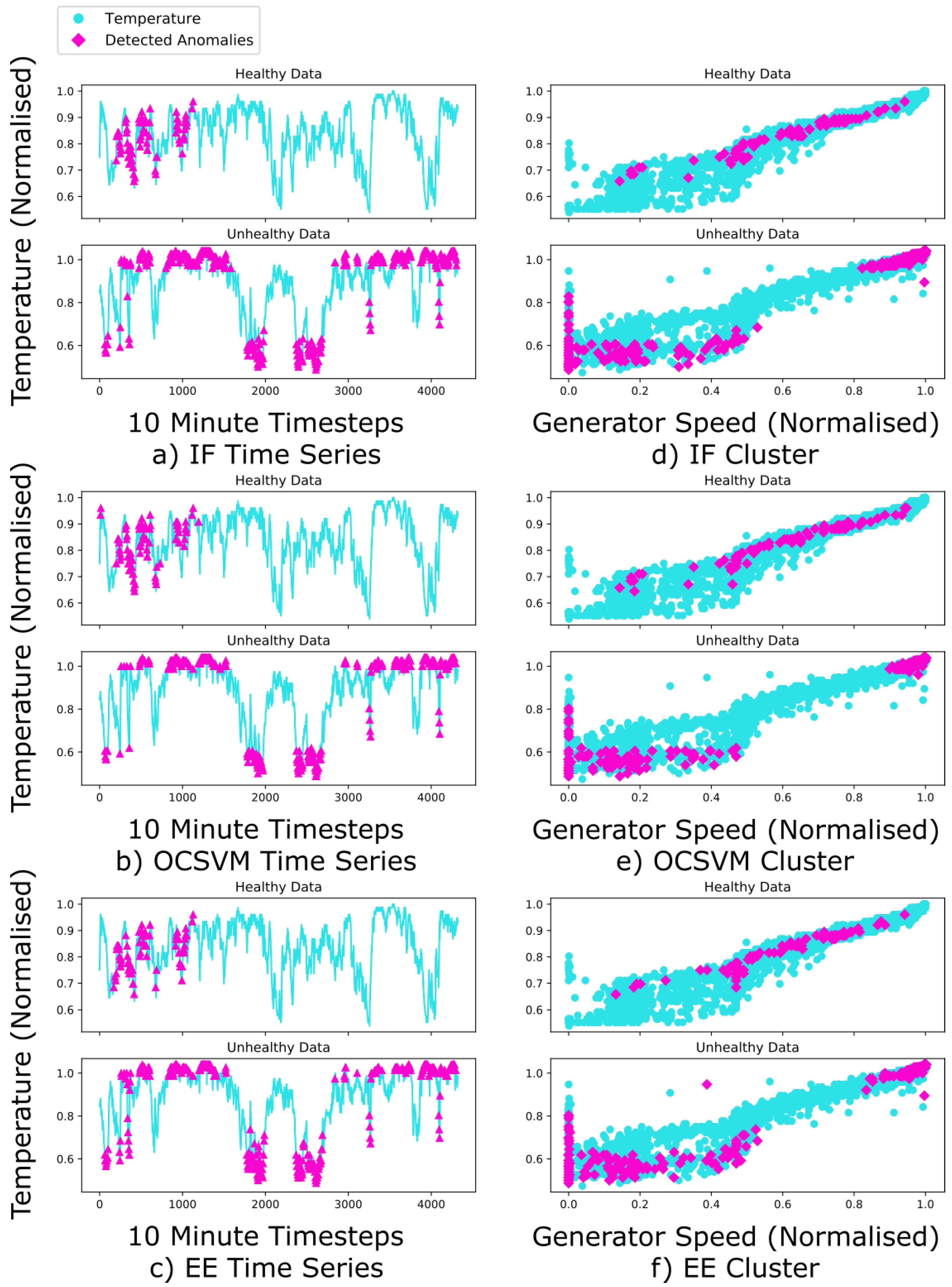
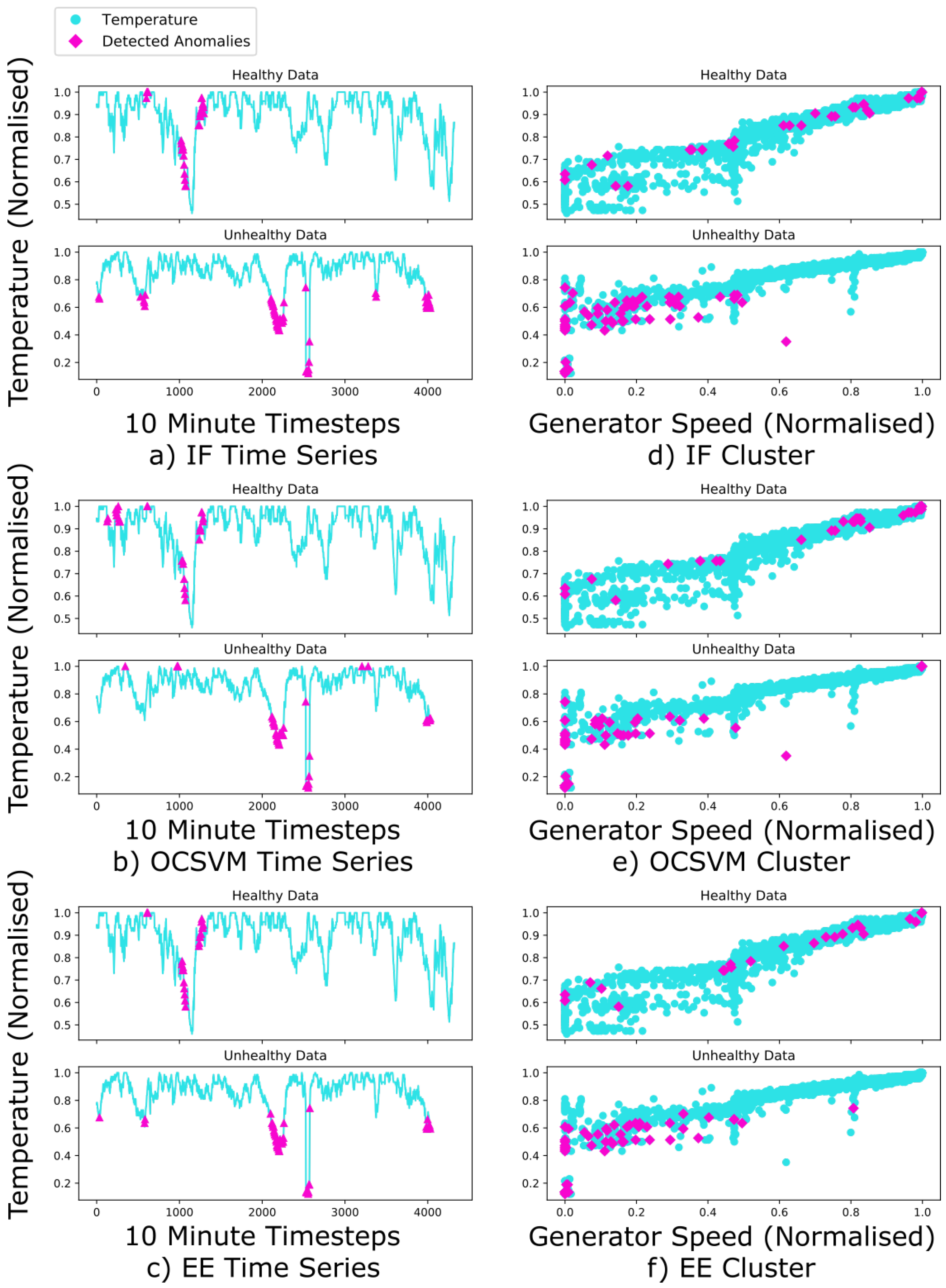
4.2. Selected Results

This section presents some examples from the tests performed in Table 4. Figure 3, Figure 4, and Figure 5a–c show the anomalies detected during both the training and testing months. Again the “healthy” data here were taken one year before failure, and the “unhealthy” data were taken one month before failure. The time series plots the Gearbox Main Bearing Temperature over the period of recording, with the anomalies overlaid when they occurred.

Figure 3, Figure 4, and Figure 5d–f show the anomalies detected on the graph of the Gearbox Main Bearing Temperature against the Generator Speed. This helps to indicate what mode of operation the anomalies tended to occur.

Figure 4 refer to the anomalies detected for turbine 3, Figure 5 is from turbine 13, and Figure 3 is from turbine 20, from different tests in Table 4. These graphs are used to help analyse the performance of the models by visualising the anomalies. It can be seen that all three models detect similar numbers of anomalies, which is consistent with the expected contamination being the same for all three models. Figure 3 is an example from a test with high IF accuracy compared to the others. Figure 4 and Figure 5 are from tests with a high accuracy for all models and low accuracy models for all respectively.

Figure 3d–f and Figure 5d–f, show a move in anomalies from higher generator speed and gearbox main bearing temperature to the lower temperatures and speeds. This can be seen partially in Figure 4d,f, where more anomalies can be seen in the lower left quadrant. This lower left quadrant was where lower temperatures and lower generator speeds occurred, and typically what would be normal operational data. This region of the cluster was typically considered normal, however in these unhealthy months there is some data considered abnormal. This consistency again could indicate unusual, or faulty, behaviour.

Figure 3, Figure 4, and Figure 5a–c show that most anomalies are detected at the extremities of the temperature values, more so at the higher temperatures. This can be expected as faults can cause increased temperature in components due to operating in a faulty regime.

It should also be noted that whilst these “cluster” plots used generator rotor speed as the x values, the generator rotor speed was not used as a feature for either the temperature or pressure target tests.

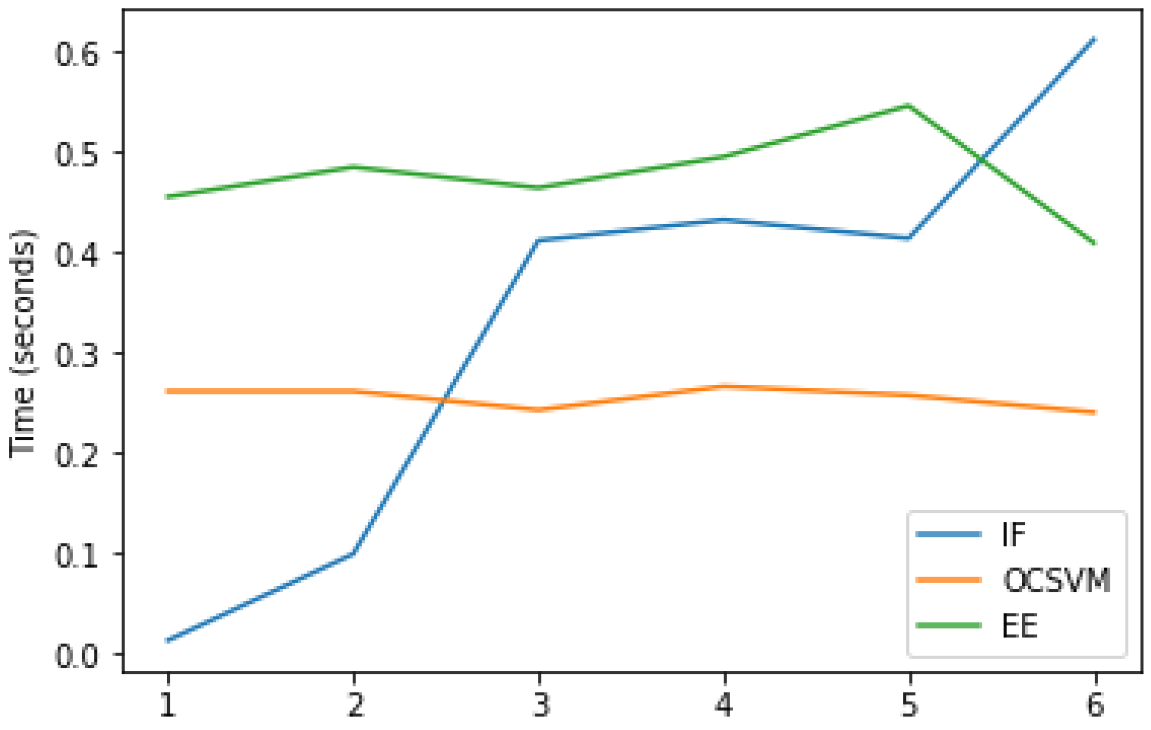
4.3. Analysis of Condition Monitoring Method

Figure 6 presents the average training times for each model for all tests conducted using each model specific hyperparameter. For example, x-value 1 shows the average training times for all IF models with one estimator, OCSVM models with a gamma value of 0.001, and EE models with a support fraction of 35%.

For the selected hyperparameters of the models, the average training times for each model can be found from Figure 6. IF average training time for 100 estimators was 432,661 microseconds, OCSVM average training time for a Gamma of 0.001 was 261,492 microseconds, and EE average training time for a support fraction of 100% was 409,726 microseconds.

Classifier models such as OCSVM, IF, or EE are appropriate for this method of condition monitoring. However performance could possibly be improved with the addition of some pre-processing steps. For example, a similar method from Zhao et al. [18] uses PCA to reduce the dimension of the input data prior to anomaly detection with support vector machine.

Anomaly detection is shown to be appropriate here as a technique for this condition monitoring method. It is shown that there is an obvious difference shown between the healthy and unhealthy months. Table 4 shows that normalised data is most appropriate for generic training as expected, as the use of multiple different turbines in one training dataset would benefit from normalising the data. The number of inputs and the target variable are not shown to affect the accuracy of the models consistently. Clean pre-processed healthy training data could be used, however for the validity of the results it may be more suitable to use raw data.

The results shown in Table 4 highlight that the generic training regime performs well considering the turbines used in this paper are located across Europe and, even though they are the same model, are different turbines. It shows that the amount of data available to train can be increased by combining data sets for multiple turbines of the same model. Further investigation is needed to find if this is viable for longer term anomaly detection also, and if this could even be extended to turbines of different models.

It would appear based on both the accuracies presented in Table 4 and Table 5, and the execution times shown in Figure 6, that OCSVM would be the best model for this form of condition monitoring. However, for future application, the specific training may be more appropriate, and therefore Isolation Forest would be the most suitable due to the greater accuracy with specific training and next lowest execution time.

In summary, this method has the potential to be an effective method of condition monitoring that utilises less data and therefore is less computationally intensive than other models that utilise longer term data. This paper looks at an effective farm of turbines where the storage and computational requirements are slightly more significant. The true benefits of reduced computational loading would come from examining fleets of turbines. Further testing of this method is needed, for a longer time period to investigate whether there would be an increasing trend in number of anomalies leading to failure. An investigation into the use of a fixed healthy month for training, and a moving test month, should be explored to show how viable the method would be for live operation.

5. Conclusions

Anomaly detection for wind turbine SCADA data is an area of active research in the wind energy community. In this paper three different outlier detection models for condition monitoring were compared. The method overall employed a data-driven approach for not just the anomaly detection but the feature selection as well. It has shown that the performance of the models varied under each of the different configurations but that Isolation Forest and OCSVM were both the most accurate of the models for both training regimes. EE was shown to perform the worst, however it was still comparable. Overall, IF and OCSVM had an average accuracy of 82% for all configurations considered, compared to 76.6% for EE. It appears that the best configuration of the data would be normalised temperature data, with four inputs trained using the generic regime. In terms of runtime, OCSVM appeared to have the shortest training time for the chosen configuration, and IF the longest.

It has been shown that the condition monitoring technique presented in this paper can be an effective assitive tool for operators and technicians for wind turbine condition monitoring. This method of condition monitoring can provide a quick snapshot of the turbine’s health, which, when monitoring the condition of a fleet of turbines, can allow an operator to quickly assess turbine health. OCSVM would be the recommended model when using a generic training regime, however as this may not be suitable for other datasets, IF would be recommended for specific training.

With the knowledge of when the turbine failed, and that each turbine failed due to the same fault, it can be assumed that the model is working correctly. With different turbine data, or different fault data, the robustness of the model could be examined in more detail. The models could then also be tested to see if they only detect this one fault, or can detect any fault within the turbine.

This initial test of the condition monitoring method has shown that anomaly detection is capable of detecting the difference in short periods of operation separated in time. Both the generic and specific training regimes have been proven to be effective. Future work will look at the investigation of a fixed reference healthy month, with a sliding test month. Comparison of this method for both a healthy turbine, and a turbine that failed during the measurement period will also be conducted for validation.

References

1. Stehly, T.; Heimiller, D.; Scott, G. 2016 Cost of Wind Energy Review; Technical Report; NREL: Golden, CO, USA, 2016.
2. Du, M.; Ma, S.; He, Q. A SCADA data based anomaly detection method for wind turbines. In Proceedings of the China International Conference on Electricity Distribution, CICED, Xi’an, China, 10–13 August 2016; pp. 1–6. [Google Scholar] [CrossRef]
3. Carroll, J.; McDonald, A.; McMillan, D. Failure rate, repair time and unscheduled O & M cost analysis of offshore wind turbines. WIND Energy 2016, 19, 1107–1119. [Google Scholar] [CrossRef]
4. Faulstich, S.; Hahn, B.; Tavner, P. Wind Turbine Downtime and its Importance for Offshore Deployment. Wind Energy 2011, 14, 327–337. [Google Scholar] [CrossRef]
5. Nielsen, J.J.; Sørensen, J.D. On risk-based operation and maintenance of offshore wind turbine components. Reliab. Eng. Syst. Saf. 2011, 96, 218–229. [Google Scholar] [CrossRef]
6. Purarjomandlangrudi, A.; Nourbakhsh, G.; Ghaemmaghami, H.; Tan, A. Application of anomaly technique in wind turbine bearing fault detection. In Proceedings of the IECON Proceedings (Industrial Electronics Conference), Dallas, TX, USA, 29 October–1 November 2014; pp. 1984–1988. [Google Scholar] [CrossRef] [Green Version]
7. Xu, X.; Lei, Y.; Zhou, X. A LOF-based method for abnormal segment detection in machinery condition monitoring. In Proceedings of the 2018 Prognostics and System Health Management Conference (PHM-Chongqing), Chongqing, China, 26–28 October 2018; pp. 125–128. [Google Scholar] [CrossRef]
8. Ogata, J.; Murakawa, M. Vibration - Based Anomaly Detection Using FLAC Features for Wind Turbine Condition Monitoring. In Proceedings of the 8th European Workshop On Structural Health Monitoring, Bilbao, Spain, 5–8 July 2016; pp. 5–8. [Google Scholar]
9. Abouel-seoud, S.A. Fault detection enhancement in wind turbine planetary gearbox via stationary vibration waveform data. J. Low Freq. Noise Vib. Act. Control 2018, 37, 477–494. [Google Scholar] [CrossRef]
10. Huitao, C.; Shuangxi, J.; Xianhui, W.; Zhiyang, W. Fault diagnosis of wind turbine gearbox based on wavelet neural network. JJ. Low Freq. Noise Vib. Act. Control 2018, 37, 977–986. [Google Scholar] [CrossRef] [Green Version]
11. Yu, D.; Chen, Z.M.; Xiahou, K.S.; Li, M.S.; Ji, T.Y.; Wu, Q.H. A radically data-driven method for fault detection and diagnosis in wind turbines. Int. J. Electr. Power Energy Syst. 2018, 99, 577–584. [Google Scholar] [CrossRef]
12. Zhao, H.; Liu, H.; Hu, W.; Yan, X. Anomaly detection and fault analysis of wind turbine components based on deep learning network. Renew. Energy 2018, 127, 825–834. [Google Scholar] [CrossRef]
13. Rezamand, M.; Kordestani, M.; Carriveau, R.; Ting, D.S.; Saif, M. A New Hybrid Fault Detection Method for Wind Turbine Blades Using Recursive PCA and Wavelet-Based PDF. IEEE Sens. J. 2020, 20, 2023–2033. [Google Scholar] [CrossRef]
14. Qu, F.; Liu, J.; Zhu, H.; Zhou, B. Wind turbine fault detection based on expanded linguistic terms and rules using non-singleton fuzzy logic. Appl. Energy 2020, 262, 114469. [Google Scholar] [CrossRef]
15. Pei, Y.; Qian, Z.; Tao, S.; Yu, H. Wind Turbine Condition Monitoring Using SCADA Data and Data Mining Method. In Proceedings of the 2018 International Conference on Power System Technology (POWERCON), Guangzhou, China, 6–8 November 2018; pp. 3760–3764. [Google Scholar]
16. Sun, Z.; Sun, H. Stacked Denoising Autoencoder With Density-Grid Based Clustering Method for Detecting Outlier of Wind Turbine Components. IEEE Access 2019, 7, 13078–13091. [Google Scholar] [CrossRef]
17. Yan, Y.; Li, J.; Gao, D.W. Condition Parameter Modeling for Anomaly Detection in Wind Turbines. Energies 2014, 7, 3104–3120. [Google Scholar] [CrossRef] [Green Version]
18. Zhao, Y.; Li, D.; Dong, A.; Lin, J.; Kang, D.; Shang, L. Fault prognosis of wind turbine generator using SCADA data. In Proceedings of the NAPS 2016—48th North American Power Symposium, Denver, CO, USA, 18–20 September 2016; pp. 1–6. [Google Scholar] [CrossRef]
19. Bangalore, P.; Letzgus, S.; Karlsson, D.; Patriksson, M. An artificial neural network-based condition monitoring method for wind turbines, with application to the monitoring of the gearbox. Wind Energy 2017, 20, 1421–1438. [Google Scholar] [CrossRef]
20. Cui, Y.; Bangalore, P.; Tjernberg, L.B. An anomaly detection approach based on machine learning and scada data for condition monitoring of wind turbines. In Proceedings of the 2018 International Conference on Probabilistic Methods Applied to Power Systems, PMAPS 2018, Boise, ID, USA, 24–28 June 2018; pp. 1–6. [Google Scholar] [CrossRef]
21. Cui, Y.; Bangalore, P.; Tjernberg, L.B. An Anomaly Detection Approach Using Wavelet Transform and Artificial Neural Networks for Condition Monitoring of Wind Turbines ’ Gearboxes. In Proceedings of the 2018 Power Systems Computation Conference (PSCC). Power Systems Computation Conference, Dublin, Ireland, 11–15 June 2018; pp. 1–7. [Google Scholar]
22. Hubert, M.; Debruyne, M.; Rousseeuw, P.J. Minimum covariance determinant and extensions. Wiley Interdiscip. Rev. Comput. Stat. 2018, 10, 1–11. [Google Scholar] [CrossRef] [Green Version]
23. Guo, K.; Liu, D.; Peng, Y.; Peng, X. Data-Driven Anomaly Detection Using OCSVM with Boundary Optimzation. In Proceedings of the 2018 Prognostics and System Health Management Conference, PHM-Chongqing 2018, Chongqing, China, 26–28 October 2008; pp. 244–248. [Google Scholar] [CrossRef]
24. Scholkopf, B.; Platt, J.C.; Shawe-Taylor, J.; Smola, A.J.; Williamson, R.C. Estimating the Support of a High-Dimensional Distribution. Neural Comput. 2001, 13, 1443–1471. [Google Scholar] [CrossRef] [PubMed]
25. Saari, J.; Strömbergsson, D.; Lundberg, J.; Thomson, A. Detection and identification of windmill bearing faults using a one-class support vector machine (SVM). Meas. J. Int. Meas. Confed. 2019, 137, 287–301. [Google Scholar] [CrossRef]
26. Wang, Y.; Yoshihashi, R.; Kawakami, R.; You, S.; Harano, T.; Ito, M.; Komagome, K.; Iida, M.; Naemura, T. Unsupervised anomaly detection with compact deep features for wind turbine blade images taken by a drone. IPSJ Trans. Comput. Vis. Appl. 2019, 11. [Google Scholar] [CrossRef]
27. Liu, F.T.; Ting, K.M. Isolation Forest. In Proceedings of the Eighth IEE International Confrence on Data Mining, Singapore, 17–20 December 2018. [Google Scholar] [CrossRef]
28. Lin, Z.; Liu, X.; Collu, M. Wind power prediction based on high-frequency SCADA data along with isolation forest and deep learning neural networks. Int. J. Electr. Power Energy Syst. 2020, 118, 105835. [Google Scholar] [CrossRef]
29. Muller, A.C.; Guido, S. Introduction to Machine Learning with Python, 1st ed.; O’Reilly: Springfield, MO, USA, 2016. [Google Scholar]
30. Gil, A.; Sanz-Bobi, M.A.; Rodríguez-López, M.A. Behavior anomaly indicators based on reference patterns - Application to the gearbox and electrical generator of a wind turbine. Energies 2018, 11, 87. [Google Scholar] [CrossRef] [Green Version]
Figure 1. Examples of the models discussed in the literature review. Figure (c) taken from [22], Wiley Interdisciplinary Reviews: Computational Statistics 2018
Energies 13 05152 g001
Figure 2. The training regimes used in this paper.
Energies 13 05152 g002
Figure 3. These figures show anomalies for the specific training regime with normalised data from the temperature target with four inputs. (ac) The blue (light) line shows the normalised main bearing temperature data. The pink (dark) triangles show when anomalies were detected during the two months. (df) The blue (light) circles shows the normalised main bearing temperature data. The pink (dark) diamonds show when anomalies were detected during the two months.
Energies 13 05152 g003
Figure 4. These figures show anomalies for the generic training regime with normalised data from the temperature target with four inputs. (ac) The blue (light) line shows the normalised main bearing temperature data. The pink (dark) triangles show when anomalies were detected during the two months. (df) The blue (light) circles shows the normalised main bearing temperature data. The pink (dark) diamonds show when anomalies were detected during the two months.
Energies 13 05152 g004
Figure 5. These figures show anomalies for the specific training regime with raw data from the temperature target with three inputs. (ac) The blue (light) line shows the normalised main bearing temperature data. The pink (dark) triangles show when anomalies were detected during the two months. (df) The blue (light) circles shows the normalised main bearing temperature data. The pink (dark) diamonds show when anomalies were detected during the two months.
Energies 13 05152 g005
Figure 6. Average execution times for each model specific hyperparameter. The values on the x-axis correspond to the case numbers in Table 3.
Energies 13 05152 g006