Joint Resource Allocation for SWIPT-Based Two-Way Relay Networks

Abstract

This paper considers simultaneous wireless information and power transfer (SWIPT) in a decode-and-forward two-way relay (DF-TWR) network, where a power splitting protocol is employed at the relay for energy harvesting. The goal is to jointly optimize power allocation (PA) at the source nodes, power splitting (PS) at the relay node, and time allocation (TA) of each duration to minimize the system outage probability. In particular, we propose a static joint resource allocation (JRA) scheme and a dynamic JRA scheme with statistical channel properties and instantaneous channel characteristics, respectively. With the derived closed-form expression of the outage probability, a successive alternating optimization algorithm is proposed to tackle the static JRA problem. For the dynamic JRA scheme, a suboptimal closed-form solution is derived based on a multistep optimization and relaxation method. We present a comprehensive set of simulation results to evaluate the proposed schemes and compare their performances with those of existing resource allocation schemes.

1. Introduction

As the Internet of Things (IoT) continues to develop, the number of low-power wireless devices connected to the Internet will increase rapidly. The energy cost for the vast amount of wireless communication and sensing devices will significantly affect the networking performance and the lifetime of nodes in IoT networks [1,2]. A promising technique to address energy issues, named simultaneous wireless information and power transfer (SWIPT), has received much attention. It is a branch of wireless energy harvesting (EH) that utilizes both the information and energy conveyed by radio frequency signals at the same time [3,4].

The concept of SWIPT was first proposed in [5] and assumed that the receiver is capable of energy harvesting and information decoding at the same time. Then, Zhou et al. [6] proposed two practical receiver architectures: time switching (TS) receiver and power splitting (PS) receiver. With these two architectures, the idea of SWIPT has been extended in many scenarios. The efficacy of SWIPT is analyzed in [7] for multiple-input single-output (MISO) systems under different channel state information (CSI), where closed-form representations of the ergodic downlink rate and the data outage probability are derived. Wirelessly powered cooperative jamming for secure communication in SWIPT systems is considered in [8], where optimal power allocation which aims at maximizing secrecy information is derived. Joint transceiver optimization is investigated in [9] for nonregenerative MIMO-SWIPT relay systems, which jointly optimizes the source precoding matrices, the relay amplification matrix, and the TS factor to maximize the source–destination mutual information (MI). In Reference [10], a “win-win” collaboration protocol is proposed for a wirelessly powered communication network (WPCN) with group cooperation. Aimed at improving the security of the primary network, the artificial-noise-aided beamforming design problems are investigated in [11] for MISO nonorthogonal multiple access (NOMA) cognitive radio networks using SWIPT.

Cooperative relay network is one of the important application scenarios to integrate SWIPT. By exploiting wireless energy harvesting, the relay node can not only extend the wireless transmission range, but also avoid consuming its own energy, which is attractive since it allows relay nodes to be battery-free. With amplify-and-forward (AF) or decode-and-forward (DF) relay protocols, SWIPT-based relay networks have gained tremendous interest. In Reference [12], the outage probability and ergodic capacity with both TS and PS protocols were derived for an AF one-way relay (OWR) network. The work in [13] investigated the TS protocol in DF-OWR fading channels, in which the ergodic throughput is maximized by jointly optimizing the mode switching and transmit power. Since two-way relay (TWR) achieves a higher spectral efficiency, increasing attention has been paid to the SWIPT-based TWR networks. In Reference [14], a SWIPT protocol for two-way AF relay was analyzed in terms of the exact expression of the outage probability, the ergodic capacity, and the finite signal-to-noise ratio (SNR) diversity-multiplexing trade-off (DMT). The work in [15] evaluates the secrecy performance of a system that employs a three-step DF-TWR with the energy harvesting capability. References [16,17] investigate the system performance in cognitive two-way networks with AF and DF protocols.

Resource allocation is a vital part of improving system performance metrics, such as energy efficiency, throughput, outage performance, etc. Joint resource allocation schemes have been wildly studied in SWIPT based relay networks recently. In [18], a resource allocation scheme is proposed for DF-OWR networks. This scheme jointly optimizes power allocation (PA), relay placement, and power splitting (PS), aiming to minimize the outage probability. In Reference [19], a joint time allocation (TA) and PS allocation scheme to improve outage performance and ergodic capacity is proposed and analyzed for SWIPT-based OWR networks. Joint resource allocation for SWIPT-based DF-TWR system is analyzed in [20], where the PS and TA ratios for the PS-based SWIPT and that of the TS and TA ratios for the TS-based SWIPT are studied to minimize the system outage probability. A joint optimal resource allocation scheme to maximize the energy efficiency (EE) is investigated for a SWIPT-enabled two-way DF relay network in [21]. In our previous studies [22], we derived the closed-form expressions of the optimal PS ratio, aimed at maximizing the achievable sum rate for DF-based SWIPT TWR network. We have also proposed a joint resource allocation scheme to minimize outage probability for DF-based SWIPT TWR network by jointly optimizing PA and PS in [23].

Of the aforementioned works, [18,19] concentrate on OWR networks. For multiple-access cases, optimization will be a lot more difficult. The studies in [20,21,22,23] are based on TWR networks. However [20,22] have not addressed PA optimization and [22,23] have not considered TA optimization. The study in [23] only analyzes dynamic resource allocation with instantaneous channel state information, in which a statistical channel state has not been taken into account. The resource allocation scheme in [21] formulates an optimization with TA, PS, and PA for the three-phase TWR network only. Moreover, the algorithm developed in the aforementioned works mainly rely on iterative techniques, and closed-form solutions of joint resource allocation have not been fully studied yet.

Inspired by the above works, we focus on the joint resource allocation (JRA) problem in a two-phase TWR network using SWIPT. The optimization work is designed to minimize the system outage probability (OP) by jointly optimizing the TA ratio, PS ratio, and PA ratio, which has not been fully studied in SWIPT-based TWR relay networks. The motivations of our work are as follows. First, closed-form solutions for JRA in a TWR network using PS energy harvesting protocol do not exist. Second, compared to AF relay, DF relay allows us to design dynamic time allocation during transmission, which increases the dimension of resource allocation, and thus improves the performance of the relay networks. Third, two-phase transmission is more appealing for TWR energy-constrained networks compared to three-phase transmission, due to its spectral efficiency. The considered system is assumed to operate at a linear EH mode, since we concentrate on the attainable theoretical performance.

The main contributions of the current work are summarized as follows:

• A comprehensive multidimension resource optimization framework to enhance the outage performance for a SWIPT-based DF-TWR network is presented, in which power allocation, power splitting, and time allocation are jointly optimized. Compared with the schemes in [20,21,22,23], the proposed scheme is more complemented and achieves better performance.
• By assuming the different availability of CSI at relay, two joint resource allocation schemes are proposed and analyzed. With statistic CSI, a successive alternating algorithm is proposed to obtain the optimal parameters based on the derived closed-form outage probability. With instantaneous CSI, a suboptimal closed-form solution of the three parameters (PS, PA, and TA) is derived based on a multistep optimization and relaxation method.
• The proposed scheme outperforms existing resource allocation schemes; for example, the dynamic JRA scheme performs very similarly to the exhaustive search method, and has better performance compared with optimal power splitting (OPS) scheme.

The remainder of the paper is organized as follows. Section 2 details the system model and the formulation of the optimization problem. In Section 3, two joint resource allocation schemes, assuming the availability of different CSI at relay, are presented and analyzed. Simulation results are presented in Section 4. Finally, we draw conclusions in Section 5.

2. System Model and Problem Formulation

2.1. System Model

Consider a DF-TWR network where two source nodes $S_1$ and $S_2$ communicate with each other via an energy harvesting relay node R, which contains a PS receiver, as shown in Figure 1. We assume there is no direct link between $S_1$ and $S_2$ due to blockage, and the relay is unwilling to use its own energy to assist the transmission. Hence, the relay can only use the harvested energy from the source signals for the information exchange. Additionally, we consider a sum power budget $P_t$ for the two transmitters $S_1$ and $S_2$ with $P_1+P_2=P_t$. Each node equipped with single antenna works in a half-duplex mode. The channels between $S_i,i=1,2$, and R are assumed to be quasi-static block Rayleigh fading, and channel reciprocity is taken into account.

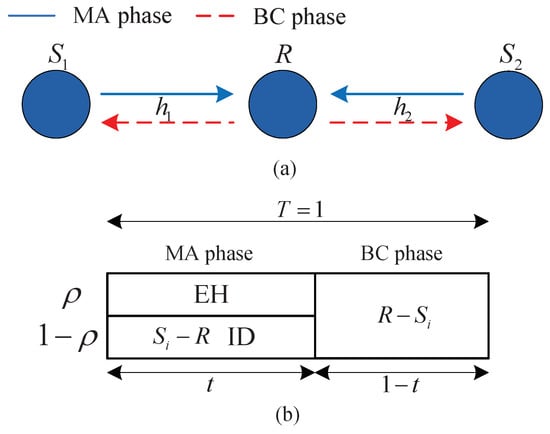
Figure 1. EH-TWR Network System Model and Transmission Structure with Power Splitting Protocol. (a) System model; (b) power splitting simultaneous wireless information and power transfer (PS-SWIPT) for decode-and-forward two-way relay (DF-TWR) network.

The whole transmission is partitioned into two phases: the first phase, named multiple-access (MA) phase; and the second phase, named broadcast (BC) phase. Denote the whole transmission time as $T=1$, the MA phase duration as t, the BC phase duration as $1-t$. In the MA phase, the two source nodes send their signals $x_i,i=1,2$ to the relay with a transmit power $P_i$. The received signal at the relay is $y_R=h_1\sqrt{P_1}{x}_1+h_2\sqrt{P_2}{x}_2+n_{r,a}$, where $E\{{\left|x_i\right|}^2\}=1$, $h_i\sim \mathcal{CN}(0,{\lambda }_i)$ is the source to relay channel coefficient, $\mathcal{CN}(·)$ denotes the complex Gaussian distribution, and $n_{r,a}\sim \mathcal{CN}(0,{\sigma }_a^2)$ is the additive noise.

The relay utilizes a power splitter to split the received signal into two parts. Let $\rho$ denote the PS ratio; the harvested energy at R during the first phase is $E=\eta \rho ({\left|h_1\right|}^2{P}_1+{\left|h_2\right|}^2{P}_2+{\sigma }_a^2)·t$, where $\eta$ is the energy conversion efficiency. The received signal at R for decoding information can be written as $y_{ID}=\sqrt{1-\rho }{y}_R+n_{r,b}$, where $n_{r,b}\sim \mathcal{CN}(0,{\sigma }^2)$ is the noise generated in the down-conversion process of the received signal [12].

In the BC phase, the relay first decodes the received signal $y_{ID}$ into $x_R=x_1\oplus x_2$ through physical layer network coding [24], then it utilizes the harvested energy to broadcast $x_R$ to source nodes $S_i$. The received signal at each source node is $y_{S_i}=h_i\sqrt{P_R}{x}_R+n_i$, where $P_R=\frac{E}{1-t}$, $n_i\sim \mathcal{CN}(0,{\sigma }_i^2)$ is the additive noise signal. Since ${\sigma }_a^2$ is much smaller compared with ${\sigma }^2$ in practice, we neglect ${\sigma }_a^2$ and consider ${\sigma }_1^2={\sigma }_2^2={\sigma }^2$ for simplicity in the following analysis (this assumption is widely assumed in research works such as [12,13,14,15,16,17,18,19,20,21,22]). Once the source node receives $y_{S_i}$, it decodes the coded information $x_R$ first, and then uses self-cancellation methods to decode the intended information. For example, the source node $S_1$ decodes the information of source node $S_2$ by $x_2=x_R\oplus x_1$.

2.2. Problem Formation

In order to assess the transmission reliability, outage performance is chosen as the metric in this manuscript. Refer to reference [25], the outage probability is denoted as the probability that the source nodes’ outage rate pair threshold $({\mathrm{R}}_{\mathrm{th}1},{\mathrm{R}}_{\mathrm{th}2})$ exceeds the achievable rate region $\mathcal{D}$ which is mathematically expressed as $P_{\mathrm{out}}=Pr[({\mathrm{R}}_{\mathrm{th}1},{\mathrm{R}}_{\mathrm{th}2})\notin \mathcal{D}]$, where $\mathcal{D}=\left\{({\mathrm{R}}_{\mathrm{th}1},{\mathrm{R}}_{\mathrm{th}2})\right|0\le {\mathrm{R}}_{12}\le min({\mathrm{R}}_{1R},{\mathrm{R}}_{R2}),0\le {\mathrm{R}}_{21}\le min({\mathrm{R}}_{2R},{\mathrm{R}}_{R1}),{\mathrm{R}}_{12}+{\mathrm{R}}_{21}\le {\mathrm{R}}_{\mathrm{MA}}\}$, ${\mathrm{R}}_{i,j},i,j\in [1,2,R]$ is the end-to-end achievable rate form node i to node j, and ${\mathrm{R}}_{\mathrm{MA}}$ is the multiple access achievable rate which is equal to the maximum supportable sum rate of the two data flows in the MA phase [20].

Denote $P_1=\alpha P_t$, $P_2=(1-\alpha )P_t$, where $0<\alpha <1$. We can obtain ${\mathrm{R}}_{i,j},i,j\in [1,2,R]$ of our system as follows according to the mathematical model given in the previous subsection:

$$\begin{array}{cc}\hfill & {\mathrm{R}}_{1R}=t·{log}_2(1+{\gamma }_{1R})\hfill \\ & {\mathrm{R}}_{R2}=(1-t)·{log}_2(1+{\gamma }_{R2})\hfill \\ & {\mathrm{R}}_{2R}=t·{log}_2(1+{\gamma }_{2R})\hfill \\ & {\mathrm{R}}_{R1}=(1-t)·{log}_2(1+{\gamma }_{R1})\hfill \\ & {\mathrm{R}}_{\mathrm{MA}}=t·{log}_2(1+{\gamma }_{\mathrm{MA}}),\hfill \end{array}$$

(1)

where ${\gamma }_{iR},i=1,2$ is the signal-to-noise ratio (SNR) from source $S_i,i=1,2$ to relay R in the MA phase; ${\gamma }_{Rj},j=1,2$ is the SNR from relay R to source $S_i,i=1,2$ in the BC phase. Thus, we have ${\gamma }_{1R}=(1-\rho )\alpha {\gamma }_1$, ${\gamma }_{2R}=(1-\rho )(1-\alpha ){\gamma }_2$, ${\gamma }_{Rj}=\frac{{\left|h_j\right|}^2\eta \rho (\alpha {\gamma }_1+(1-\alpha ){\gamma }_2)·t}{1-t},j=1,2$, ${\gamma }_{\mathrm{MA}}={\gamma }_{1R}+{\gamma }_{2R}=(1-\rho )(\alpha {\gamma }_1+(1-\alpha ){\gamma }_2)$, where ${\gamma }_1=\frac{{\left|h_1\right|}^2{P}_t}{{\sigma }^2}$, ${\gamma }_2=\frac{{\left|h_2\right|}^2{P}_t}{{\sigma }^2}$.

By substituting Equation (1) into $P_{\mathrm{out}}=Pr[({\mathrm{R}}_{\mathrm{th}1},{\mathrm{R}}_{\mathrm{th}2})\notin \mathcal{D}]$, the outage probability of the system is rewritten as

$$\begin{array}{cc}\hfill P_{out}=& Pr\{min({\mathrm{R}}_{1R},{\mathrm{R}}_{R2})<{\mathrm{R}}_{\mathrm{th}1},\mathrm{or}min({\mathrm{R}}_{2R},{\mathrm{R}}_{R1})<{\mathrm{R}}_{\mathrm{th}2}\hfill \\ & \mathrm{or}{\mathrm{R}}_{\mathrm{MA}}<{\mathrm{R}}_{\mathrm{th}1}+{\mathrm{R}}_{\mathrm{th}2}\}\hfill \\ \hfill =& Pr\{{\gamma }_{1R}<{\gamma }_{\mathrm{th}1}^t\mathrm{or}{\gamma }_{R2}<{\gamma }_{\mathrm{th}1}^{1-t}\mathrm{or}{\gamma }_{2R}<{\gamma }_{\mathrm{th}2}^t\hfill \\ & \mathrm{or}{\gamma }_{R1}<{\gamma }_{\mathrm{th}2}^{1-t},\mathrm{or}{\gamma }_{\mathrm{MA}}<{\gamma }_{\mathrm{th}\Sigma }^t\}\hfill \\ \hfill =& Pr\left\{min\left(\frac{{\gamma }_{1R}}{{\gamma }_{\mathrm{th}1}^t},\frac{{\gamma }_{R2}}{{\gamma }_{\mathrm{th}1}^{1-t}},\frac{{\gamma }_{2R}}{{\gamma }_{\mathrm{th}2}^t},\frac{{\gamma }_{R1}}{{\gamma }_{\mathrm{th}2}^{1-t}},\frac{{\gamma }_{\mathrm{MA}}}{{\gamma }_{\mathrm{th}\Sigma }^t}\right)<1\right\},\hfill \end{array}$$

(2)

where $Pr\left\{x\right\}$ is the probability formula of x, ${\gamma }_{\mathrm{th}i}^t=2^{\frac{{\mathrm{R}}_{\mathrm{th}i}}{t}}-1$, ${\gamma }_{\mathrm{th}i}^{1-t}=2^{\frac{{\mathrm{R}}_{\mathrm{th}i}}{1-t}}-1$, $i=1,2$, ${\gamma }_{\mathrm{th}\Sigma }^t$ = $2^{\frac{{\mathrm{R}}_{\mathrm{th}1}+{\mathrm{R}}_{\mathrm{th}2}}{t}}-1$.

Denote the generalized signal-to-noise ratio (SNR) as $\Lambda =min\left(\frac{{\gamma }_{1R}}{{\gamma }_{\mathrm{th}1}^t},\frac{{\gamma }_{R2}}{{\gamma }_{\mathrm{th}1}^{1-t}},\frac{{\gamma }_{2R}}{{\gamma }_{\mathrm{th}2}^t},\frac{{\gamma }_{R1}}{{\gamma }_{\mathrm{th}2}^{1-t}},\frac{{\gamma }_{\mathrm{MA}}}{{\gamma }_{\mathrm{th}\Sigma }^t}\right)$. The outage probability can be rewritten as

$$\begin{array}{c}\hfill P_{out}=Pr\{\Lambda <1\}=F_{\Lambda }\left(1\right),\end{array}$$

(3)

where $F_X(·)$ is the cumulative distribution function (CDF) of X. Note that the power allocation at the source nodes, power splitting at the relay node, and time allocation at each duration all affect on the outage probability. To better illustrate the relationship among them, we rewrite the outage probability as $P_{out}=P_{out}(\alpha ,\rho ,t)$. Then, an optimization problem to minimize the system outage probability by optimizing the three parameters is formulated as

$$\begin{array}{c}\hfill \mathbf{OP}\mathbf{0}:({\alpha }^o,{\rho }^o,t^o)=argmin{P}_{out}(\alpha ,\rho ,t)\\ \hfill \mathrm{s}.\mathrm{t}.0<\alpha <1,0<\rho <1,0<t<1.\end{array}$$

(4)

3. Joint Resource Allocation Schemes

In this section, we focus on designing the optimal transmission in terms of minimum outage probability by jointly optimizing the PS, PA, and TA ratios. Two resource allocation schemes are proposed and analyzed: static transmission scheme to minimize the outage probability when statistical CSI is known; and dynamic transmission scheme to maximize the generalized SNR when instantaneous CSI is known.

3.1. Optimal Static JRA Scheme

To optimize the JRA scheme based on statistical CSI in terms of outage performance, we derive the closed-form expression of the outage probability first. From Equation (3), we have

$$\begin{array}{c}\hfill P_{out}=F_{\Lambda }\left(1\right)=1-{\tilde{F}}_{\Lambda }\left(1\right),\end{array}$$

(5)

where

$$\begin{array}{cc}\hfill {\tilde{F}}_{\Lambda }\left(1\right)=& Pr\{\Lambda \ge 1\}\hfill \\ \hfill =& Pr\{\frac{(1-\rho )\alpha {\gamma }_1}{{\gamma }_{\mathrm{th}1}^t}\ge 1,\frac{|h_2{|}^2\eta \rho (\alpha {\gamma }_1+(1-\alpha ){\gamma }_2)t}{{\gamma }_{\mathrm{th}1}^{1-t}(1-t)}\ge 1,\hfill \\ & \frac{(1-\rho )(1-\alpha ){\gamma }_2}{{\gamma }_{\mathrm{th}2}^t}\ge 1,\frac{|h_1{|}^2\eta \rho (\alpha {\gamma }_1+(1-\alpha ){\gamma }_2)t}{{\gamma }_{\mathrm{th}2}^{1-t}(1-t)}\ge 1,\hfill \\ & \frac{(1-\rho )(\alpha {\gamma }_1+(1-\alpha ){\gamma }_2)}{{\gamma }_{\mathrm{th}\Sigma }^t}\ge 1\}.\hfill \end{array}$$

(6)

Denote $X_1=\alpha {\gamma }_1$ and $X_2=(1-\alpha ){\gamma }_2$. Equation (6) can be rewritten as

$$\begin{array}{cc}\hfill {\tilde{F}}_{\Lambda }\left(1\right)=& Pr\{X_1\ge a_1,X_2\ge a_2,\hfill \\ & X_1+X_2\ge max\left(a_3,\frac{b_1}{X_2},\frac{b_2}{X_1}\right)\}\hfill \\ \hfill =& \sum _{i=0}^{2}Pr\left\{E_i\right\},\hfill \end{array}$$

(7)

where $a_1=\frac{{\gamma }_{\mathrm{th}1}^t}{1-\rho }$, $a_2=\frac{{\gamma }_{\mathrm{th}2}^t}{1-\rho }$, $a_3=\frac{{\gamma }_{\mathrm{th}\Sigma }^t}{1-\rho }$, $b_1=\frac{(1-\alpha )P_t·{\gamma }_{\mathrm{th}1}^{1-t}·(1-t)}{\eta \rho {\sigma }^{2}t}$, $b_2=\frac{\alpha P_t·{\gamma }_{\mathrm{th}2}^{1-t}·(1-t)}{\eta \rho {\sigma }^{2}t}$, and

$$\begin{array}{cc}\hfill E_0=& \{X_1\ge max\left(a_1,\frac{b_2}{a_3}\right),X_2\ge max\left(a_2,\frac{b_1}{a_3}\right),\hfill \\ & X_1+X_2\ge a_3\}\hfill \\ \hfill E_1=& \{X_1\ge max\left(a_1,\frac{b_1}{X_2}-X_2,\frac{b_2}{b_1}{X}_2\right),\hfill \\ & a_2\le X_2\le \frac{b_1}{a_3}\}\hfill \\ \hfill E_2=& \{X_2\ge max\left(a_2,\frac{b_2}{X_1}-X_1,\frac{b_1}{b_2}{X}_1\right),\hfill \\ & a_1\le X_1\le \frac{b_2}{a_3}\}.\hfill \end{array}$$

(8)

Since the channels obey Rayleigh fading and $h_1\sim \mathcal{CN}(0,{\lambda }_1)$, $h_2\sim \mathcal{CN}(0,{\lambda }_2)$, the probability density function of random variables $X_1$ and $X_2$ can be written as

$$\begin{array}{cc}\hfill & f_{X_1}\left(x_1\right)={\Omega }_1·\exp \left(-{\Omega }_1·x_1\right)\hfill \\ & f_{X_2}\left(x_2\right)={\Omega }_2·\exp \left(-{\Omega }_2·x_2\right),\hfill \end{array}$$

(9)

where ${\Omega }_1={({\lambda }_1\alpha P_t/{\sigma }^2)}^{-1}$, ${\Omega }_2={({\lambda }_2(1-\alpha )P_t/{\sigma }^2)}^{-1}$. According to the former equations, Theorem 1 is obtained as follows.

Theorem 1.

When the channels obey Rayleigh fading, the system outage probability is

$$\begin{array}{cc}\hfill P_{out}=& 1-I\left(max\left(a_1,\frac{b_2}{a_3}\right),max\left(a_2,\frac{b_1}{a_3}\right),a_3\right)\hfill \\ & -\sum _{i=1}^2{V}_i\left(a_i,b_i,\frac{b_{3-i}}{b_i},a_{3-i},\frac{b_i}{a_3}\right),\hfill \end{array}$$

(10)

where $I\left(max\left(a_1,\frac{b_2}{a_3}\right),max\left(a_2,\frac{b_1}{a_3}\right),a_3\right)$ is the probability of event $E_0$, $V_i\left(a_i,b_i,\frac{b_{3-i}}{b_i},a_{3-i},\frac{b_i}{a_3}\right)$ are the probability of event $E_i,i=1,2$, respectively, and

$$I(y_1,y_2,y_3)=\left\{\begin{array}{c}{e}^{-{\Omega }_1{y}_1}·e^{-{\Omega }_2{y}_2},y_1+y_2\ge y_3\hfill \\ \sum _{i=1}^2\frac{{\Omega }_i}{{\omega }_i-{\Omega }_{3-i}}{e}^{-{\Omega }_i{y}_i-{\Omega }_{3-i}·(y_3-y_i)}\hfill \\ ,y_1+y_2<y_3,{\Omega }_1\ne {\Omega }_2\hfill \\ e^{-{\Omega }_1{y}_3}(1+{\Omega }_1{y}_3-{\Omega }_1{y}_1-{\Omega }_1{y}_2)\hfill \\ ,y_1+y_2<y_3,{\Omega }_1={\Omega }_2\hfill \end{array}\right.$$

(11)

$$\begin{array}{cc}\hfill & V_i\left(a_i,a_{3-i},b_i,\frac{b_i}{a_3},\frac{b_{3-i}}{b_i}\right)\hfill \\ \hfill =& Q_i\left(a_i,max\left(a_{3-i},\sqrt{\frac{a_i^2}{4}+b_i}-\frac{a_i}{2}\right),min\left(\frac{b_i}{a_3},\frac{a_i{b}_i}{b_{3-i}}\right)\right)\hfill \\ & +U_i\left(\frac{b_{3-i}}{b_i}{X}_{3-i},max\left(a_{3-i},\frac{a_i{b}_i}{b_{3-i}},\frac{b_i}{\sqrt{b_i+b_{3-i}}}\right),\frac{b_i}{a_3}\right)\hfill \\ & +W_i\left(\frac{b_i}{X_{3-i}}-X_{3-i},a_{3-i},min\left(\frac{b_i}{a_3},\sqrt{\frac{a_i^2}{4}+b_i}-\frac{a_i}{2},\frac{b_i}{\sqrt{b_i+b_{3-i}}}\right)\right).\hfill \end{array}$$

(12)

The three components of Equation (12) ($Q_i$, $U_i$, and $W_i$) can be calculated by the following three equations, respectively:

$$\begin{array}{cc}\hfill & Q_i(q_{i1},q_{i2},q_{i3})=e^{-{\Omega }_i{q}_{i1}}·\left(e^{-{\Omega }_{3-i}{q}_{i2}}-e^{-{\Omega }_{3-i}{q}_{i3}}\right)\hfill \\ \hfill & U_i(u_{i1}{X}_{3-i},u_{i2},u_{i3})=\frac{{\Omega }_{3-i}}{{\Omega }_{3-i}+{\Omega }_i{u}_{i1}}\left(e^{-({\Omega }_{3-i}+{\Omega }_i{u}_{i1})u_{i2}}-e^{-({\Omega }_{3-i}+{\Omega }_i{u}_{i1})u_{i3}}\right)\hfill \\ \hfill & W_i(\frac{w_{i1}}{X_{3-i}}-X_{3-i},w_{i2})\approx {\Omega }_{3-i}\frac{w_{i3}}{2}\varpi \sum _{n=1}^N\sqrt{1-{\varphi }_n^2}·e^{-({\Omega }_{3-i}-{\Omega }_i)c_{i3}-\frac{{\Omega }_i{w}_{i1}}{c_{i3}}}\hfill \\ & -{\Omega }_{3-i}\frac{w_{i2}}{2}\varpi \sum _{n=1}^N\sqrt{1-{\varphi }_n^2}·e^{-({\Omega }_{3-i}-{\Omega }_i)d_{i2}-\frac{{\Omega }_i{w}_{i1}}{d_{i2}}}\hfill \end{array}$$

(13)

where $\varpi =\frac{\pi }{N}$, ${\varphi }_n=cos\left(\frac{2n-1}{2N}\pi \right)$, $c_{i3}=\frac{w_{i3}}{2}(1+\varphi )$, $d_{i2}=\frac{w_{i2}}{2}(1+\varphi )$, and N is a parameter to ensure the complexity–accuracy trade-off.

Proof. 

The proof is given in Appendix A. □

Equation (10) shows that the closed-form outage probability expression is a nonconvex function in terms of $\alpha$, $\rho$, and t jointly, from which we cannot directly derive the optimal values of $\alpha$, $\rho$, and t. We propose a successive alternating optimization (SAO) algorithm to solve this joint optimization problem. The algorithm steps are listed below:

Step 1, initialize the parameters $\rho$, t, and $P_{out}^{\mathrm{pre}}=1$;

Step 2, with the updated $\rho$ and t, obtain $\alpha$ by doing one-dimension numerical search: $\alpha$ = $\underset{0<\alpha <1}{argmin}{P}_{out}$;

Step 3, update t and $\alpha$, obtain $\rho$ by doing one-dimension numerical search: $\rho =\underset{0<\rho <1}{argmin}{P}_{out}$;

Step 4, update $\rho$ and $\alpha$, obtain t by doing one-dimension numerical search: $t=\underset{0<t<1}{argmin}{P}_{out}$;

Step 5, calculate $P_{out}^{\mathrm{cur}}$ with current $\alpha$, $\rho$, and t. If $|P_{out}^{\mathrm{cur}}-P_{out}^{\mathrm{pre}}|>\epsilon$, return to Step 2 and update $P_{out}^{\mathrm{pre}}=P_{out}^{\mathrm{cur}}$;

Step 6, if $|P_{out}^{\mathrm{cur}}-P_{out}^{\mathrm{pre}}|<\epsilon$, then stop and record the final $P_{out}^{\mathrm{cur}}$, t, $\rho$, and $\alpha$.

The algorithm has a double-layer loop. Step 2–Step 4 are inner loop, in which each one-dimensional numerical search has a computational complexity of $\mathcal{O}\left(N\right)$. Steps 5 and 6 are the outer loop, which have a computational complexity of $\mathcal{O}\left(N\right)$ as well. Thus, the computational complexity of the proposed algorithm is $\mathcal{O}\left(N^2\right)$ due to the use of successive alternating optimization.

3.2. Optimal Dynamic JRA Scheme

In this subsection, we investigate the optimization design of the JRA scheme based on instantaneous CSI from the perspective of the generalized SNR. The optimization problem in Equation (4) is equivalent to maximizing the generalized SNR when each node knows the instantaneous CSI. The equivalent optimization problem is written as

$$\begin{array}{c}\hfill \mathbf{OP}\mathbf{1}:({\alpha }^o,{\rho }^o,t^o)=argmax\Lambda (\alpha ,\rho ,t)\\ \hfill \mathrm{s}.\mathrm{t}.0\le \alpha \le 1,0\le \rho \le 1,0\le t\le 1.\end{array}$$

(14)

Equation (2) shows that $\Lambda$ is a complex function of $\alpha$, $\rho$, and t. To avoid the complex process of directly solving for a solution, we propose a multistep optimization algorithm. The process is depicted as follows.

In the first step, we fix the variables $\alpha$ and t. The optimization problem decomposes to a one-dimensional optimization problem which is determined by $\rho$ only:

$$\begin{array}{cc}\hfill \mathbf{OP}\mathbf{2}:& {\rho }^o=argmax\Lambda \left(\rho \right)\hfill \\ & \mathrm{s}.\mathrm{t}.0\le \rho \le 1.\hfill \end{array}$$

(15)

$\Lambda \left(\rho \right)$ can be rewritten as $\Lambda \left(\rho \right)=min\left((1-\rho )g_1(\alpha ,t),\rho g_2(\alpha ,t)\right)$, where

$$\begin{array}{cc}\hfill & g_1(\alpha ,t)=min\left(\frac{\alpha {\gamma }_1}{2^{\frac{{\mathrm{R}}_{\mathrm{th}1}}{t}}-1},\frac{(1-\alpha ){\gamma }_2}{2^{\frac{{\mathrm{R}}_{\mathrm{th}2}}{t}}-1},\frac{\alpha {\gamma }_1+(1-\alpha ){\gamma }_2}{2^{\frac{{\mathrm{R}}_{\mathrm{th}\Sigma }}{t}}-1}\right)\hfill \\ & g_2(\alpha ,t)=min\left(\frac{|h_2{|}^2}{2^{\frac{{\mathrm{R}}_{\mathrm{th}1}}{1-t}}-1},\frac{|h_1{|}^2}{2^{\frac{{\mathrm{R}}_{\mathrm{th}2}}{1-t}-1}}\right)·\frac{\eta (\alpha {\gamma }_1+(1-\alpha ){\gamma }_2)t}{1-t}.\hfill \end{array}$$

(16)

It is observed that $(1-\rho )g_1(\alpha ,t)$ and $\rho g_2(\alpha ,t)$ are a monotonically decreasing function and a monotonically increasing function, respectively, according to Equation (16). Thus, the optimal solution of $\mathbf{OP}\mathbf{2}$ can be obtained at $(1-\rho )g_1(\alpha ,t)=\rho g_2(\alpha ,t)$, which is

$$\begin{array}{c}\hfill {\rho }^o=\frac{g_1(\alpha ,t)}{g_1(\alpha ,t)+g_2(\alpha ,t)}.\end{array}$$

(17)

Substituting the obtained ${\rho }^o$ back into $\Lambda$, the original optimization problem becomes a two-dimensional optimization problem, which is affected by $\alpha$ and t, and its objective function $\Lambda$ becomes

$$\begin{array}{c}\hfill \Lambda (\alpha ,t)=\frac{g_1(\alpha ,t)·g_2(\alpha ,t)}{g_1(\alpha ,t)+g_2(\alpha ,t)}.\end{array}$$

(18)

Since the objective function $\Lambda (\alpha ,t)$ is nonconvex, we then utilize a two-step optimization algorithm to solve it. Firstly, we derive the closed-form of optimal PA ratio $\alpha$ by fixing TA ratio t; then, we derive the closed-form of TA ratio t with fixed PA ratio $\alpha$, where the derived closed-form of TA ratio t is verified to be a static value; finally, we substitute the derived static value of t back into the first step and obtain the final optimal $\alpha$. The derivation is explained next.

3.2.1. Optimal PA When TA Is Fixed

When fixing t, $\Lambda (\alpha ,t)$ decomposes to a one-dimensional function $\Lambda \left(\alpha \right)$. Let $\overline{\Lambda }\left(\alpha \right)=\frac{1}{g_1\left(\alpha \right)}+\frac{1}{g_2\left(\alpha \right)}$, the optimization problem can be found as

$$\begin{array}{cc}\hfill \mathbf{OP}\mathbf{3}:& \left({\alpha }^o\right)=argmin\overline{\Lambda }\left(\alpha \right)\hfill \\ & =argmin\left(\frac{1}{g_1\left(\alpha \right)}+\frac{1}{g_2\left(\alpha \right)}\right)\hfill \\ & \mathrm{s}.\mathrm{t}.0\le \alpha \le 1.\hfill \end{array}$$

(19)

Denote $q_1=\frac{{\gamma }_{\mathrm{th}1}^t}{\alpha {\gamma }_1}$, $q_2=\frac{{\gamma }_{\mathrm{th}2}^t}{(1-\alpha ){\gamma }_2}$, $q_3=\frac{{\gamma }_{\mathrm{th}\Sigma }^t}{\alpha {\gamma }_1+(1-\alpha ){\gamma }_2}$, and let ${\alpha }_{12}$, ${\alpha }_{13}$, ${\alpha }_{23}$ denote the intersection points for $\{(q_1,q_2),(q_1,q_3),(q_2,q_3)\}$. Comparing the values of ${\alpha }_{13}$ and ${\alpha }_{23}$ reveals that $\overline{\Lambda }\left(\alpha \right)$ can be classified into the following two cases:

Case 1: ${\alpha }_{13}\ge {\alpha }_{23}$

$$\overline{\Lambda }\left(\alpha \right)=\left\{\begin{array}{c}{q}_1+v^{-1}·{(\alpha {\gamma }_1+(1-\alpha ){\gamma }_2)}^{-1},0<\alpha \le {\alpha }_{12}\hfill \\ q_2+v^{-1}·{(\alpha {\gamma }_1+(1-\alpha ){\gamma }_2)}^{-1},{\alpha }_{12}<\alpha <1\hfill \end{array}\right.$$

(20)

Case 2: ${\alpha }_{13}<{\alpha }_{23}$

$$\overline{\Lambda }\left(\alpha \right)=\left\{\begin{array}{c}{q}_1+v^{-1}·{(\alpha {\gamma }_1+(1-\alpha ){\gamma }_2)}^{-1},0<\alpha \le {\alpha }_{13}\hfill \\ q_3+v^{-1}·{(\alpha {\gamma }_1+(1-\alpha ){\gamma }_2)}^{-1},{\alpha }_{13}<\alpha \le {\alpha }_{23}\hfill \\ q_2+v^{-1}·{(\alpha {\gamma }_1+(1-\alpha ){\gamma }_2)}^{-1},{\alpha }_{23}<\alpha <1,\hfill \end{array}\right.$$

(21)

where $v=\eta ·min\left(\frac{|h_2{|}^2}{{\gamma }_{\mathrm{th}1}^{1-t}},\frac{|h_1{|}^2}{{\gamma }_{\mathrm{th}2}^{1-t}}\right)·\frac{t}{1-t}$, ${\alpha }_{12}=\frac{{\gamma }_2{\gamma }_{\mathrm{th}1}^t}{{\gamma }_1{\gamma }_{\mathrm{th}2}^t+{\gamma }_2{\gamma }_{\mathrm{th}1}^t}$, ${\alpha }_{13}=\frac{{\gamma }_2{\gamma }_{\mathrm{th}1}^t}{{\gamma }_1({\gamma }_{\mathrm{th}\Sigma }^t-{\gamma }_{\mathrm{th}1}^t)+{\gamma }_2{\gamma }_{\mathrm{th}1}^t}$, ${\alpha }_{23}=$ $\frac{{\gamma }_2({\gamma }_{\mathrm{th}\Sigma }^t-{\gamma }_{\mathrm{th}2}^t)}{{\gamma }_2({\gamma }_{\mathrm{th}\Sigma }^t-{\gamma }_{\mathrm{th}2}^t)+{\gamma }_1{\gamma }_{\mathrm{th}2}^t}$.

Analyzing $\overline{\Lambda }\left(\alpha \right)$ provided in Equations (20) and (21), we notice that it is a continuous convex segmented function. Based on the two derived cases of $\overline{\Lambda }\left(\alpha \right)$, the optimal PA ratio ${\alpha }^o$ with fixed TA ratio t can be obtained as shown in the following Theorem 2.

Theorem 2.

When fixing TA ratio t, the optimal PA ratio ${\alpha }^o$ is

$${\alpha }^o=\left\{\begin{array}{c}{\alpha }_{12},{\gamma }_1={\gamma }_2\hfill \\ {\alpha }_{\mathrm{case}1}^{\ast },{\gamma }_1>{\gamma }_2,{\alpha }_{13}\ge {\alpha }_{23}\hfill \\ {\alpha }_{\mathrm{case}2}^{\ast },{\gamma }_1>{\gamma }_2,{\alpha }_{13}<{\alpha }_{23}\hfill \\ {\alpha }_{\mathrm{case}1}^{+},{\gamma }_1<{\gamma }_2,{\alpha }_{13}\ge {\alpha }_{23}\hfill \\ {\alpha }_{\mathrm{case}2}^{+},{\gamma }_1<{\gamma }_2,{\alpha }_{13}<{\alpha }_{23}\hfill \end{array}\right.$$

(22)

where ${\alpha }_{\mathrm{case}1}^{\ast }=max({\alpha }^{\ast },{\alpha }_{12})$, ${\alpha }_{\mathrm{case}2}^{\ast }=max({\alpha }^{\ast },{\alpha }_{23})$, ${\alpha }_{\mathrm{case}1}^{+}=min({\alpha }^{+},{\alpha }_{12})$, ${\alpha }_{\mathrm{case}2}^{+}=min({\alpha }^{+},{\alpha }_{13})$, and

$$\begin{array}{cc}\hfill & {\alpha }^{\ast }=\frac{\sqrt{{\gamma }_2({\gamma }_1-{\gamma }_2)}-{\gamma }_2\sqrt{v{\gamma }_{\mathrm{th}2}^t}}{\sqrt{{\gamma }_2({\gamma }_1-{\gamma }_2)}+({\gamma }_1-{\gamma }_2)\sqrt{v{\gamma }_{\mathrm{th}2}^t}}\hfill \\ & {\alpha }^{+}=\frac{{\gamma }_{\mathrm{th}1}^{t}v{\gamma }_2({\gamma }_2-{\gamma }_1)-{\gamma }_2\sqrt{v{\gamma }_1{\gamma }_{\mathrm{th}1}^t({\gamma }_2-{\gamma }_1)}}{({\gamma }_2-{\gamma }_1)(v{\gamma }_{\mathrm{th}1}^t({\gamma }_2-{\gamma }_1)-{\gamma }_1)}.\hfill \end{array}$$

(23)

Proof. 

The proof is given in Appendix B. □

3.2.2. Optimal TA When PA Is Fixed

In this part, we use relaxation method to obtain the approximating closed-form of t with fixed $\alpha$. Since $g_1(\alpha ,t)$, $g_2(\alpha ,t)$ have exponential functions of t, in order to simplify the derivation and obtain the closed-form, we use the following values as the approximate expression of $g_1(\alpha ,t)$, $g_2(\alpha ,t)$:

$$\begin{array}{cc}\hfill & {\tilde{g}}_1(\alpha ,t)=min\left(\frac{\alpha {\gamma }_1}{2^{\frac{{\mathrm{R}}_{\mathrm{th}1}}{t}}},\frac{(1-\alpha ){\gamma }_2}{2^{\frac{{\mathrm{R}}_{\mathrm{th}2}}{t}}},\frac{\alpha {\gamma }_1+(1-\alpha ){\gamma }_2}{2^{\frac{{\mathrm{R}}_{\mathrm{th}\Sigma }}{t}}}\right)\hfill \\ & {\tilde{g}}_2(\alpha ,t)=min\left(\frac{|h_2{|}^2}{2^{\frac{{\mathrm{R}}_{\mathrm{th}1}}{1-t}}},\frac{|h_1{|}^2}{2^{\frac{{\mathrm{R}}_{\mathrm{th}2}}{1-t}}}\right)·\frac{\eta (\alpha {\gamma }_1+(1-\alpha ){\gamma }_2)t}{1-t}.\hfill \end{array}$$

(24)

We rewrite the elements in ${\tilde{g}}_1(\alpha ,t)$ as $\frac{A_j}{2^{\frac{{\mathrm{R}}_{\mathrm{th}j}}{t}}}$, where each element of ${\tilde{g}}_1(\alpha ,t)$ corresponds to $\left(A_j,{\mathrm{R}}_{\mathrm{th}j}\right)\in \left\{(\alpha {\gamma }_1,{\mathrm{R}}_{\mathrm{th}1}),((1-\alpha ){\gamma }_2,{\mathrm{R}}_{\mathrm{th}2}),(\alpha {\gamma }_1+(1-\alpha ){\gamma }_2,{\mathrm{R}}_{\mathrm{th}\Sigma })\right\}$. We also rewrite ${\tilde{g}}_2(\alpha ,t)=\frac{|h_{3-i}{|}^2}{2^{\frac{{\mathrm{R}}_{\mathrm{th}i}}{1-t}}}·\frac{\eta (\alpha {\gamma }_1+(1-\alpha ){\gamma }_2)t}{1-t}$ for any elements of ${\tilde{g}}_2(\alpha ,t)$, where $i=1,2$.

With the rewritten ${\tilde{g}}_1(\alpha ,t)$ and ${\tilde{g}}_2(\alpha ,t)$, the objective function $\tilde{\Lambda }(\alpha ,t)$ can be rewritten as

$$\begin{array}{cc}\hfill \tilde{\Lambda }(\alpha ,t)& =\frac{{\tilde{g}}_1(\alpha ,t)·{\tilde{g}}_2(\alpha ,t)}{{\tilde{g}}_1(\alpha ,t)+{\tilde{g}}_2(\alpha ,t)}\hfill \\ & =\frac{\frac{A_j}{2^{\frac{{\mathrm{R}}_{\mathrm{th}j}}{t}}}·\frac{|h_{3-i}{|}^2}{2^{\frac{{\mathrm{R}}_{\mathrm{th}i}}{1-t}}}·\frac{\eta (\alpha {\gamma }_1+(1-\alpha ){\gamma }_2)t}{1-t}}{\frac{A_j}{2^{\frac{{\mathrm{R}}_{\mathrm{th}j}}{t}}}·\frac{|h_{3-i}{|}^2}{2^{\frac{{\mathrm{R}}_{\mathrm{th}i}}{1-t}}}+\frac{\eta (\alpha {\gamma }_1+(1-\alpha ){\gamma }_2)t}{1-t}}\hfill \\ & =\frac{A_j{\left|h_{3-i}\right|}^2\eta (\alpha {\gamma }_1+(1-\alpha ){\gamma }_2)}{A_j{2}^{\frac{{\mathrm{R}}_{\mathrm{th}i}}{1-t}}·\frac{1-t}{t}+{\left|h_{3-i}\right|}^2·\eta (\alpha {\gamma }_1+(1-\alpha ){\gamma }_2)·2^{\frac{{\mathrm{R}}_{\mathrm{th}j}}{t}}}.\hfill \end{array}$$

(25)

It can be noticed that the denominator of $\tilde{\Lambda }(\alpha ,t)$ obtained in Equation (25) is a convex function in terms of t, and the numerator is a constant. Thus, the maximum value of $\tilde{\Lambda }(\alpha ,t)$ can be obtained when the denominator of $\tilde{\Lambda }(\alpha ,t)$ is minimum. Consider that the second part of the denominator includes the channel coefficient ${\left|h_{3-i}\right|}^2$, which will become very small when the path loss is high. Therefore, when severe path loss is taken into account, the objective function $\tilde{\Lambda }(\alpha ,t)$ has a tight upper-bound, expressed as

$$\begin{array}{c}\hfill \tilde{\Lambda }(\alpha ,t)\le \frac{A_j{\left|h_{3-i}\right|}^2\eta (\alpha {\gamma }_1+(1-\alpha ){\gamma }_2)}{A_j{2}^{\frac{{\mathrm{R}}_{\mathrm{th}i}}{1-t}}·\frac{1-t}{t}}.\end{array}$$

(26)

Analyzing the tight upper-bound, Theorem 3 is obtained as follows.

Theorem 3.

When fixing PA ratio α, the optimal TA ratio $t^o$ is

when $|h_1{|}^2>{\left|h_2\right|}^2$,

$$t^o=\left\{\begin{array}{c}{t}_1,t_1<t_0\hfill \\ t_0,t_2<t_0<t_1\hfill \\ t_2,t_2>t_0\hfill \end{array}\right.$$

(27)

when ${\left|h_1\right|}^2\le {\left|h_2\right|}^2$,

$$t^o=\left\{\begin{array}{c}{t}_2,t_2<t_0\hfill \\ t_0,t_1<t_0<t_2\hfill \\ t_1,t_1>t_0\hfill \end{array}\right.$$

(28)

where $t_0=1-\frac{({\mathrm{R}}_{\mathrm{th}2}-{\mathrm{R}}_{\mathrm{th}1})ln2}{ln|h_1{|}^2-ln{\left|h_2\right|}^2}$, $t_1=\frac{1}{{\mathrm{R}}_{\mathrm{th}1}·ln2+1}$, $t_2=\frac{1}{{\mathrm{R}}_{\mathrm{th}2}·ln2+1}$.

Proof. 

The proof is given in Appendix C. □

As can be seen, with relaxation method, the optimal TA ratio $t^o$ in terms of fixing PA ratio $\alpha$ is a constant, i.e., not affected by $\alpha$. Thus, the final optimal TA ratio of $\Lambda (\alpha ,t)$ is the obtained value $t^o$. With the obtained $t^o$, the final optimal PA ratio ${\alpha }^o$ can be obtained by Equation (22). With the obtained $t^o$ and ${\alpha }^o$, the final optimal PS ratio ${\rho }^o$ can be derived by Equation (17). The algorithm is a multistep optimization with relaxation method (MO-RM), which is utilized to obtain the closed-form of all three parameters $t^o$, ${\alpha }^o$, and ${\rho }^o$ as follows:

Step 1, we obtain the optimal time allocation ratio $t^o$ by utilizing Equations (27) and (28);

Step 2, update $t=t^o$, then obtain the optimal power allocation by utilizing Equation (22);

Step 3, update $t=t^o$ and $\alpha ={\alpha }^o$, then obtain the optimal power splitting by utilizing Equation (17).

The algorithm mainly consists of a set of comparisons to calculate $t^o$, which can be realized by a set of comparators; the computation required to calculate $t_0$, $t_1$, $t_2$, ${\alpha }^o$, and ${\rho }^o$ is insignificant.

4. Simulation Results

In this section, numerical results are provided to verify the theoretical analysis derived in the previous section, and the performance of the investigated network using the two JRA schemes are examined. Moreover, three baseline schemes—i.e., equal resource allocation (ERA) scheme, optimal power splitting (OPS) scheme [20,22], and joint optimal power splitting and power allocation (JOPSPA) scheme [19,23]—are compared with the two proposed JRA schemes. The characteristics of the involved resource allocation schemes are listed in Table 1. In the simulation, the distance between the two sources is set to $d=10$ m and the relay is positioned on a straight line connecting the two sources such that $d_1+d_2=d$, where $d_i,i=1,2$ is the distance between $S_i$ and R [20]. Energy conversion efficiency $\eta$ is set to be $\eta =0.8$, which has been widely adopted to explore the performance of SWIPT-enabled systems, such as [13,20,22]. We assume $h_i\sim \mathcal{CN}(0,\frac{1}{d_i^m})$ with pass loss exponent $m=2.5$, and noise variances are set to be ${\sigma }^2={10}^{-7}$ W.

Table 1. Characteristics of different resource allocation schemes. ERA—equal resource allocation; OPS—optimal power splitting; JOPSPA—joint optimal power splitting and power allocation; JRA—joint resource allocation; CSI—channel state information.

Schemes	Characteristic
ERA	$t=0.5$, $\alpha =0.5$, and $\rho =0.5$
OPS	$t=0.5$, $\alpha =0.5$, and $\rho ={\rho }^o$ [20,22]
JOPSPA	$t=0.5$, $\alpha ={\alpha }^o$, and $\rho ={\rho }^o$ [19,23]
Static JRA	Jointly optimizing t, $\alpha$, and $\rho$ with statistical CSI
Dynamic JRA	Jointly optimizing t, $\alpha$, and $\rho$ with instantaneous CSI

Figure 2 shows the effect of N (the coefficient that affects the closed-form of $W_i$ in Equation (13c)) on the closed-form outage probability derived for the static JRA scheme at $({\mathrm{R}}_{\mathrm{th}1},{\mathrm{R}}_{\mathrm{th}2})=$ $\left\{\right(0.5,2),(0.5,1\left)\right\}$ bit/s/Hz and $d_1=\{3,5\}$ m. The results are obtained from Equation (10) with N as the x-axis. The parameters PA ratio $\alpha$, PS ratio $\rho$, and TA ratio t are all set to 0.5. It is observed that the outage probability remains stable when N increases to a certain value, and a small N is sufficient to make the outage probability reach the stable value. Thus, we can use small N to obtain outage probability in the following simulations.

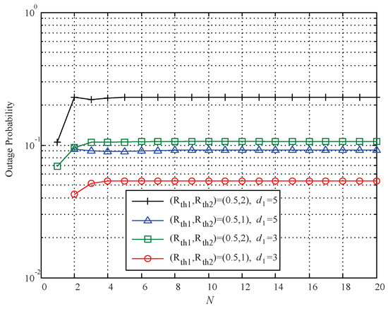
Figure 2. Effects of N on the outage probability for static JRA scheme.

Figure 3 depicts the curves of outage probability against PA ratio $\alpha$, TA ratio t, or PS ratio $\rho$ with $N=\{20,200\}$. The outage probability in this figure is obtained by numerical search with Equation (10) and Monte Carlo simulation with Equation (3). It can be seen that the theoretical results obtained by numerical search with Equation (10) coincide with the Monte Carlo simulation results in all regions, which verifies the correctness of the derivation of Equation (10). It also shows that the outage probability is not a monotonic function of the PA ratio, PS ratio, or TA ratio, that is, there is one and only one minimum outage probability for any variables when fixing another two parameters.

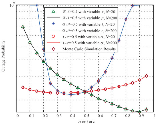
Figure 3. Outage probability vs. PA ratio $\alpha$, TA ratio t, or PS ratio $\rho$.

In the following figures, we assess the proposed optimal allocation schemes. Each curve is generated from ${10}^4$ channel realizations. The outage probability of static JRA scheme is obtained by Equation (10), and the outage probability of dynamic JRA scheme is obtained by Equation (3) with Monte Carlo simulations. For static JRA scheme, the optimal parameters ${\alpha }^o$, $t^o$, and ${\rho }^o$ utilized in outage probability calculation are calculated by SAO algorithm. For dynamic JRA scheme, the parameters ${\alpha }^o$, $t^o$, and ${\rho }^o$ utilized in the outage probability calculation are calculated by MO-RM algorithm.

Figure 4 compares the outage probability of the two proposed JRA schemes (optimal static JRA scheme and optimal dynamic JRA scheme) with the optimal schemes obtained by exhaustive search (ES). From the curves, as the total power budget $P_t$ increases, the optimal outage performance of each scheme decreases. It can be seen that the static JRA scheme has a similar outage performance compared with the ES scheme (ES with statistical channel properties), whereas the dynamic JRA scheme has a slightly worse performance, i.e., it it approaches the performance of the ES scheme (ES with instantaneous channel properties) under various conditions. This is because the dynamic JRA scheme is based on relaxation method, which will decrease the outage performance. The figure also depicts that the dynamic JRA scheme enjoys better performance than the static JRA scheme. This is because the optimal parameters of the static JRA scheme are stable, while the dynamic JRA scheme is able to adjust the optimal parameters with instantaneous CSI which will contribute to the outage performance.

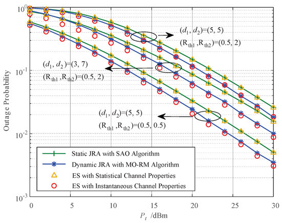
Figure 4. Comparison of the two proposed JRA schemes with the exhaustive search schemes. SAO—successive alternating optimization; MO-RM—multistep optimization with relaxation method; ES—exhaustive search.

The outage probability of the proposed static JRA scheme versus the total power budget $P_t$ is presented in Figure 5, and is compared with three other schemes—JOPSPA, OPS, and ERA—based on statistical CSI with different relay deployments, i.e., $(d_1,d_2)=(5,5)$ m and $(d_1,d_2)=(3,7)$ m. It can be seen that all the four schemes have a decreasing outage probability with the increase of $P_t$. Further, the proposed static JRA scheme enjoys the best performance compared with the other three schemes, followed by the JOPSPA scheme, the OPS scheme, and the ERA scheme for each relay deployment case, especially at high power budgets or high rate thresholds. The advantage of the static JRA scheme is evident, since it can make full use of the resource of power and time compared with the other schemes. However, in the peer scheme, the assigned time or power is equal. Moreover, the outage performance of the proposed static JRA scheme increases as the target rate arises. This is because when the target rate is low, there is less power needed for decoding information at relay and shorter time needed for the first phase, which results in more power for harvesting and more time for second phase transmission.

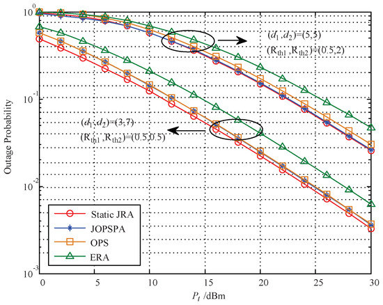
Figure 5. Outage probability vs. $P_t$ based on statistic CSI. OPS—optimal power splitting.

The outage probability of the proposed dynamic JRA scheme versus the total power budget $P_t$ is depicted in Figure 6, compared with three other schemes—JOPSPA, OPS, and ERA—based on instantaneous CSI with different replay deployments, i.e., $(d_1,d_2)=(5,5)$ m and $(d_1,d_2)=(3,7)$ m. It can be seen that the outage performance obtained by the proposed dynamic JRA scheme outperforms the ERA scheme, the OPS scheme, and the JOPSPA scheme for each relay deployment case. The reason is the same as above (see analysis in Figure 5). In addition, the outage performance shown in Figure 6 is slightly worse than that in Figure 5 for the same scheme. This is because with the instantaneous CSI, the system can adjust their parameters which can contribute to the outage performance.

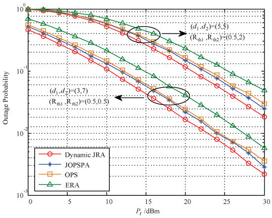
Figure 6. Outage probability vs. $P_t$ based on instantaneous CSI.

Figure 7 presents the optimal outage probability versus the relay deployment with two cases of rate threshold pair $\left\{({\mathrm{R}}_{\mathrm{th}1},{\mathrm{R}}_{\mathrm{th}2})\right|(0.5,0.5),(0.5,2)\}$ for the four resource allocation schemes based on statistical CSI (we use $d_1$, the distance between $S_1$ and $S_2$, as the x-axis). It can be seen that the proposed static JRA scheme outperforms the other schemes in all $d_1$ regions. All the curves in terms of $d_1$ present a concave function, which exhibits the worst performance when $d_1\approx 5$ for the symmetric rates and when $d_1\in (5,9)$ for asymmetric rates due to the energy harvesting capability. The phenomenon showing the best performance is related to the relay location and rate pair threshold.

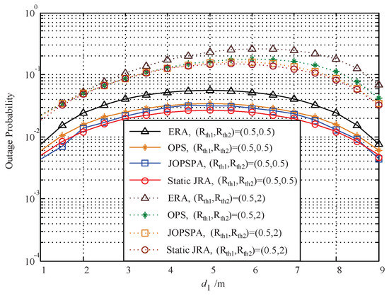
Figure 7. Outage probability vs. $d_1$ based on statistic CSI.

Figure 8 presents the optimal outage probability versus the relay deployment (the x-axis is $d_1$) for the four resource allocation schemes based on instantaneous CSI. It can be seen that the proposed static JRA scheme outperforms the other schemes in all $d_1$ regions, and increasing the distance between source $S_1$ and relay (i.e., $d_1$) leads to a concave characteristic and exhibits the worst performance with different relay deployment settings for symmetric and asymmetric rates. The outage performance shown in Figure 8 is slightly worse than that in Figure 7 for the same scheme, owing to the system’s ability to adjust its parameters with the instantaneous CSI.

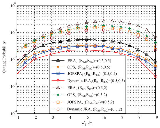
Figure 8. Outage probability vs. $d_1$ based on instantaneous CSI.

5. Conclusions

In this paper, two JRA schemes for DF-TWR relaying networks with SWIPT are studied based on statistical and instantaneous CSI from the perspective of the outage performance, respectively. For the static JRA scheme, we first derive the closed-form outage probability expressions and then tackle the joint optimization of TS, PS, and TA through a successive alternating optimization algorithm. For the dynamic JRA scheme, we utilize the multistep optimization and relaxation method to obtain a suboptimal closed-form solution of TS, PS, and TA. The analytical results are verified via extensive simulation results. The proposed JRA schemes have been found to outperform three benchmark schemes—ERA, OPS, and JOPSPA schemes—which provide a basis for the optimization of EH-TWR systems. Further work could study hybrid energy harvesting schemes such as the one proposed in [26] for this TWR scenario. It is also interesting to design UAV-based energy harvesting schemes similar to those in [27,28] for relay systems.

References

- Fadi, A.; Enver, E.; Hadi, Z. Small Cells in the Forthcoming 5G/IoT: Traffic Modelling and Deployment Overview. IEEE Commun. Surv. Tutor. 2019, 21, 28–65. [Google Scholar]
- Kamalinejad, P.; Mahapatra, C.; Sheng, Z.; Mirabbasi, S.; Leung, V.C.M.; Guan, L.Y. Wireless Energy Harvesting for the Internet of Things. IEEE Commun. Mag. 2015, 53, 102–108. [Google Scholar] [CrossRef]
- Li, M.L.; Chen, Y.; Liu, K.J.R. Advances in Energy Harvesting Communications: Past, Present, and Future Challenges. IEEE Commun. Surv. Tutor. 2016, 18, 1384–1412. [Google Scholar]
- Louie, R.; Li, Y.; Vucetic, B. A Survey on Simultaneous Wireless Information and Power Transfer With Cooperative Relay and Future Challenges. IEEE Access 2019, 7, 19166–19198. [Google Scholar]
- Varshney, L.R. Transporting Information and Energy Simultaneously. In Proceedings of the IEEE International Symposium on Information Theory, Toronto, ON, Canada, 6–11 July 2008. [Google Scholar]
- Zhou, X.; Zhang, R.; Ho, C.K. Wireless Information and Power Transfer: Architecture Design and Rate-Energy Tradeoff. IEEE Trans. Commun. 2013, 63, 4754–4767. [Google Scholar] [CrossRef]
- Liu, C.; Maso, M.; Lakshminarayana, S.; Lee, C.; Quek, T.Q.S. Simultaneous Wireless Information and Power Transfer Under Different CSI Acquisition Schemes. IEEE Trans. Wirel. Commun. 2015, 14, 1911–1926. [Google Scholar] [CrossRef]
- Liu, M.; Liu, Y. Power Allocation for Secure SWIPT Systems With Wireless-Powered Cooperative Jamming. IEEE Commun. Lett. 2017, 21, 1353–1356. [Google Scholar] [CrossRef]
- Li, B.; Rong, Y. Joint Transceiver Optimization for Wireless Information and Energy Transfer in Nonregenerative MIMO Relay Systems. IEEE Trans. Wirel. Commun. 2018, 67, 8348–8362. [Google Scholar] [CrossRef]
- Xiong, K.; Chen, C.; Qu, G.; Fan, P. Group Cooperation With Optimal Resource Allocation in Wireless Powered Communication Networks. IEEE Trans. Wirel. Commun. 2017, 16, 3840–3853. [Google Scholar] [CrossRef]
- Zhou, F.; Chu, Z.; Sun, H.; Hu, R.Q.; Hanzo, L. Artificial Noise Aided Secure Cognitive Beamforming for Cooperative MISO-NOMA Using SWIPT. IEEE J. Sel. Areas Commun. 2018, 36, 918–931. [Google Scholar] [CrossRef]
- Nasir, A.A.; Zhou, X.; Durrani, S.; Kennedy, R.A. Relaying Protocols for Wireless Energy Harvesting and Information Processing. IEEE Trans. Wirel. Commun. 2013, 12, 3622–3636. [Google Scholar] [CrossRef]
- Tang, L.; Zhang, X.; Zhu, P.; Wang, X. Wireless Information and Energy Transfer in Fading Relay Channels. IEEE J. Sel. Areas Commun. 2016, 34, 3632–3645. [Google Scholar] [CrossRef]
- Chen, Z.; Xia, B.; Liu, H. Wireless information and power transfer in two-way amplify-and-forward relaying channels. In Proceedings of the IEEE Global Conference on Signal and Information Processing (GlobalSIP), Atlanta, GA, USA, 3–5 December 2014; pp. 168–172. [Google Scholar]
- Jameel, F.; Wyne, S.; Ding, Z. Secure Communications in Three-Step Two-Way Energy Harvesting DF Relaying. IEEE Commun. Lett. 2018, 22, 308–311. [Google Scholar] [CrossRef]
- Singh, S.; Modem, S.; Prakriya, S. Optimization of Cognitive Two-Way Networks With Energy Harvesting Relays. IEEE Commun. Lett. 2017, 21, 1381–1384. [Google Scholar] [CrossRef]
- Nguyen, D.K.; Jayakody, D.N.K.; Chatzinotas, S.; Thompson, J.S.; Li, J. Wireless Energy Harvesting Assisted Two-Way Cognitive Relay Networks: Protocol Design and Performance Analysis. IEEE Access 2017, 5, 21447–21460. [Google Scholar] [CrossRef]
- Mishra, D.; De, S.; Chiasserini, C. Joint Optimization Schemes for Cooperative Wireless Information and Power Transfer Over Rician Channels. IEEE Trans. Commun. 2016, 64, 554–571. [Google Scholar] [CrossRef]
- Ye, Y.; Li, Y.; Wang, D.; Zhou, F.; Hu, R.Q.; Zhang, H. Optimal Transmission Schemes for DF Relaying Networks Using SWIPT. IEEE Trans. Veh. Tech. 2018, 67, 7062–7072. [Google Scholar] [CrossRef]
- Do, T.P.; Song, I.; Kim, Y.H. Simultaneous Wireless Transfer of Power and Information in a Decode-and-Forward Two-Way Relaying Network. IEEE Trans. Wirel. Commun. 2017, 16, 1579–1592. [Google Scholar] [CrossRef]
- Shi, L.; Ye, Y.; Hu, R.Q.; Zhang, H. Energy Efficiency Maximization for SWIPT Enabled Two-Way DF Relaying. IEEE Signal Process. Lett. 2019, 26, 755–759. [Google Scholar] [CrossRef]
- Peng, C.; Li, F.; Liu, H. Optimal power splitting in two-way decode-and-forward relay networks. IEEE Commun. Lett. 2017, 21, 2009–2012. [Google Scholar] [CrossRef]
- Peng, C.; Li, F.; Liu, H.; Wang, G. Outage-Based Resource Allocation for DF Two-Way Relay Networks with Energy Harvesting. Sensors 2018, 18, 3496. [Google Scholar] [CrossRef] [PubMed]
- Zhang, S.; Liew, S.C.; Lu, L. Physical Layer Network Coding Schemes over Finite and Infinite Fields. In Proceedings of the IEEE Global Telecommunications Conference, New Orleans, LO, USA, 30 November–4 December 2008. [Google Scholar]
- Liu, P.; Kim, I.M. Performance analysis of bidirectional communication protocols based on decode-and-forward relaying. IEEE Trans. Commun. 2010, 58, 2683–2696. [Google Scholar] [CrossRef]
- Altinel, D.; Kurt, G.K. Modeling of Multiple Energy Sources for Hybrid Energy Harvesting IoT Systems. IEEE Internet Things J. 2019, 6, 10846–10854. [Google Scholar] [CrossRef]
- Yin, S.; Zhao, Y.; Li, L.; Yu, F.R. UAV-Assisted Cooperative Communications With Time-Sharing Information and Power Transfer. IEEE Trans. Veh. Tech. 2020, 69, 1554–1567. [Google Scholar] [CrossRef]
- Jayakody, D.N.K.; Perera, T.D.P.; Ghrayeb, A.; Hasna, M.O. Self-Energized UAV-Assisted Scheme for Cooperative Wireless Relay Networks. IEEE Trans. Veh. Tech. 2020, 69, 578–592. [Google Scholar] [CrossRef]
Publisher’s Note: MDPI stays neutral with regard to jurisdictional claims in published maps and institutional affiliations. |
© 2020 by the authors. Licensee MDPI, Basel, Switzerland. This article is an open access article distributed under the terms and conditions of the Creative Commons Attribution (CC BY) license (http://creativecommons.org/licenses/by/4.0/).