Simulation and Measurement of Energetic Performance in Decentralized Regenerative Ventilation Systems

 , ,
, ,
Abstract
1. Introduction
2. Methodology
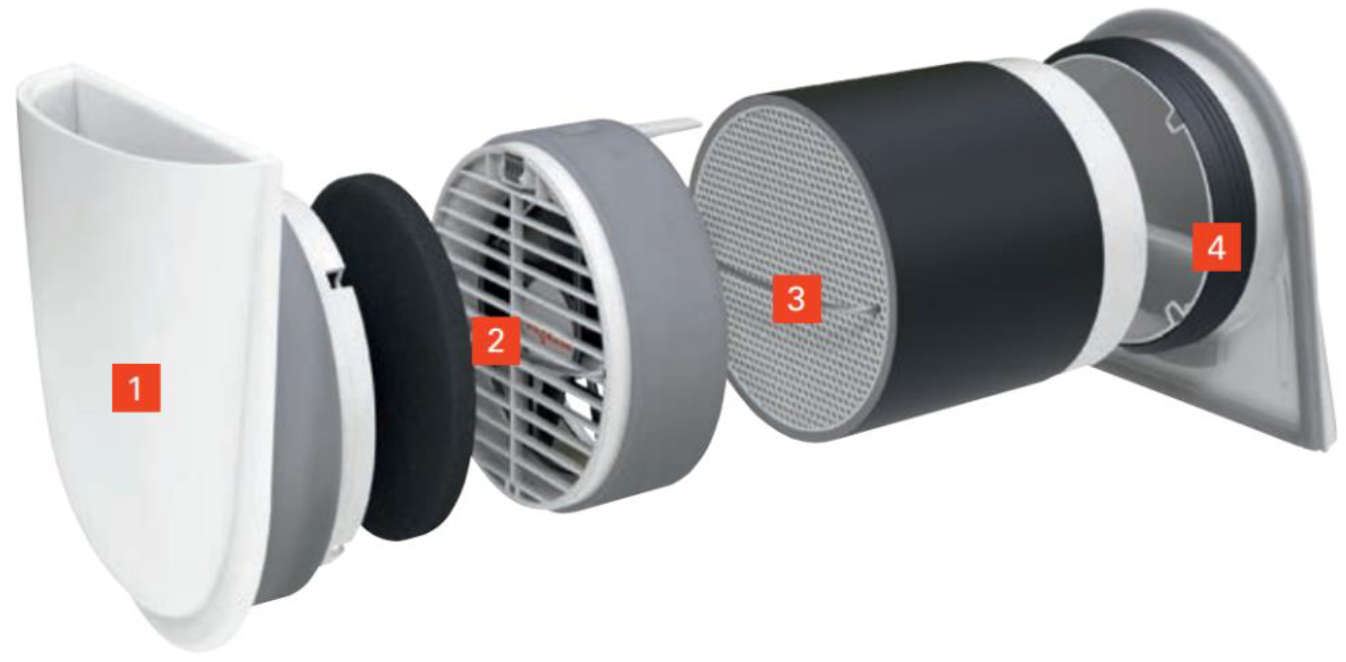
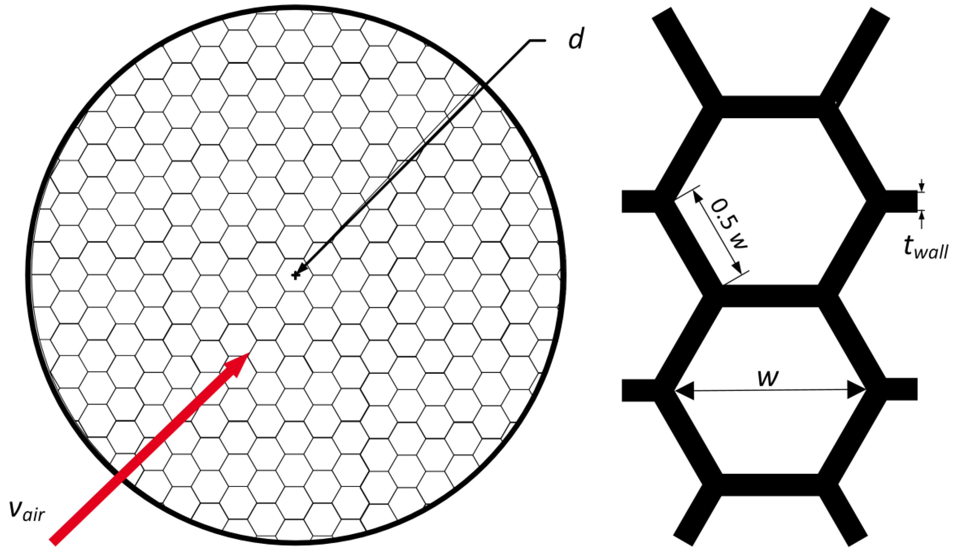
2.1. Heat Exchanger
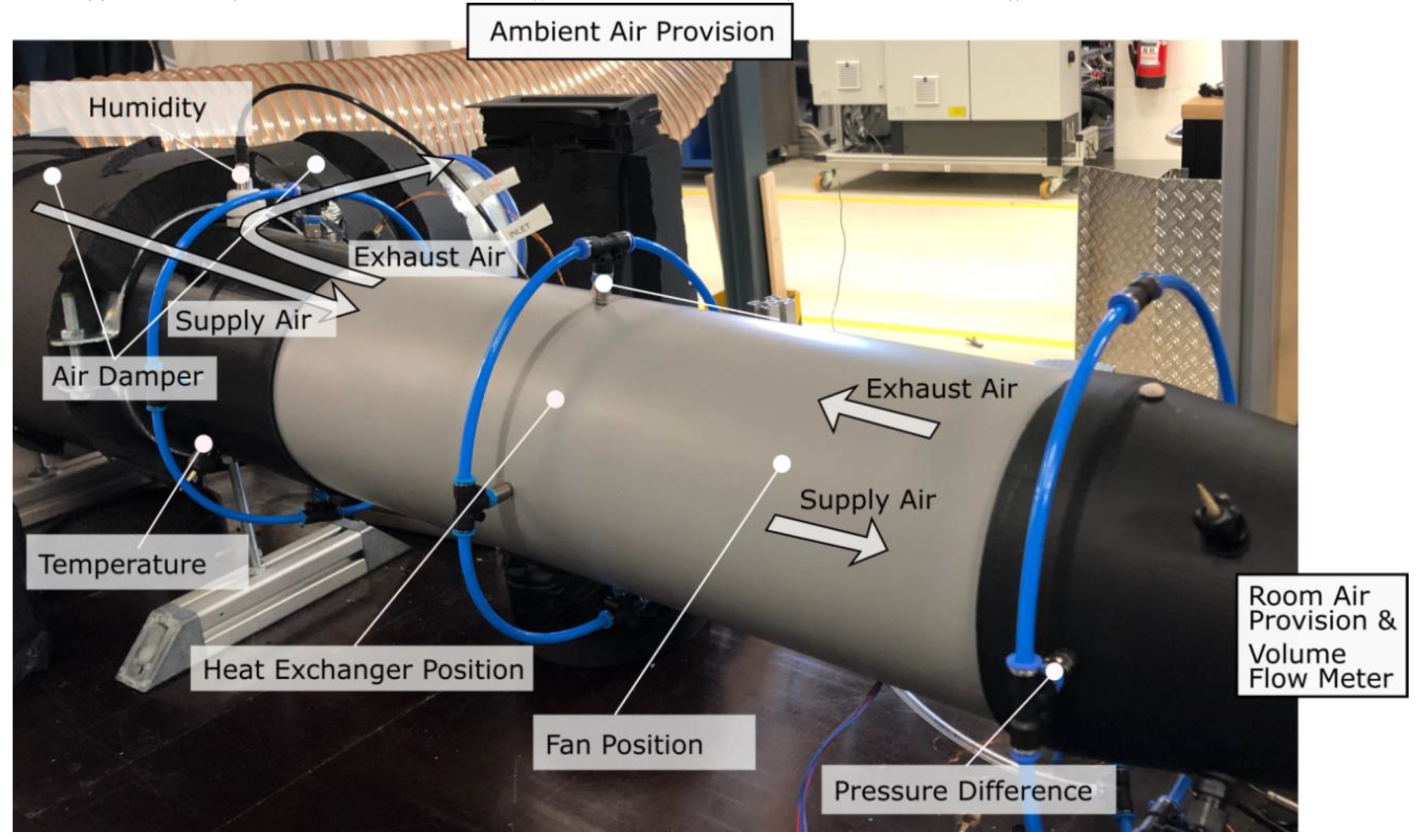
2.2. Laboratory Test Facility
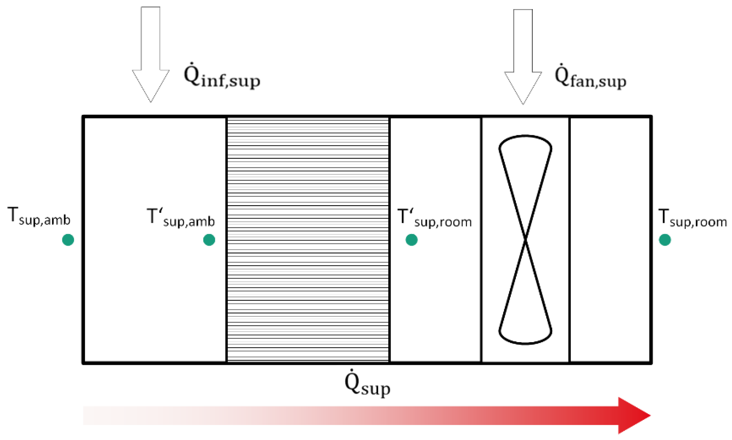
2.3. Thermal Model
2.3.1. Finite Element Method for CFD
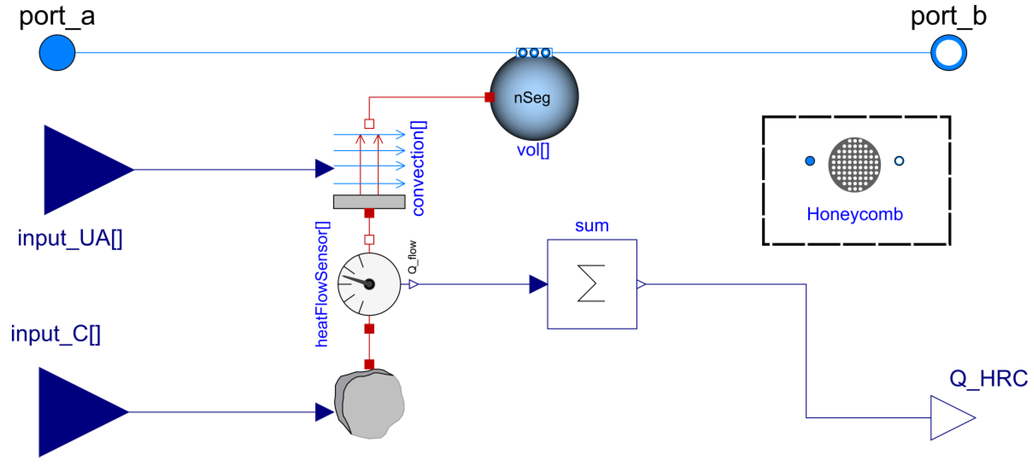
2.3.2. Dynamic 1D Model Using Modelica
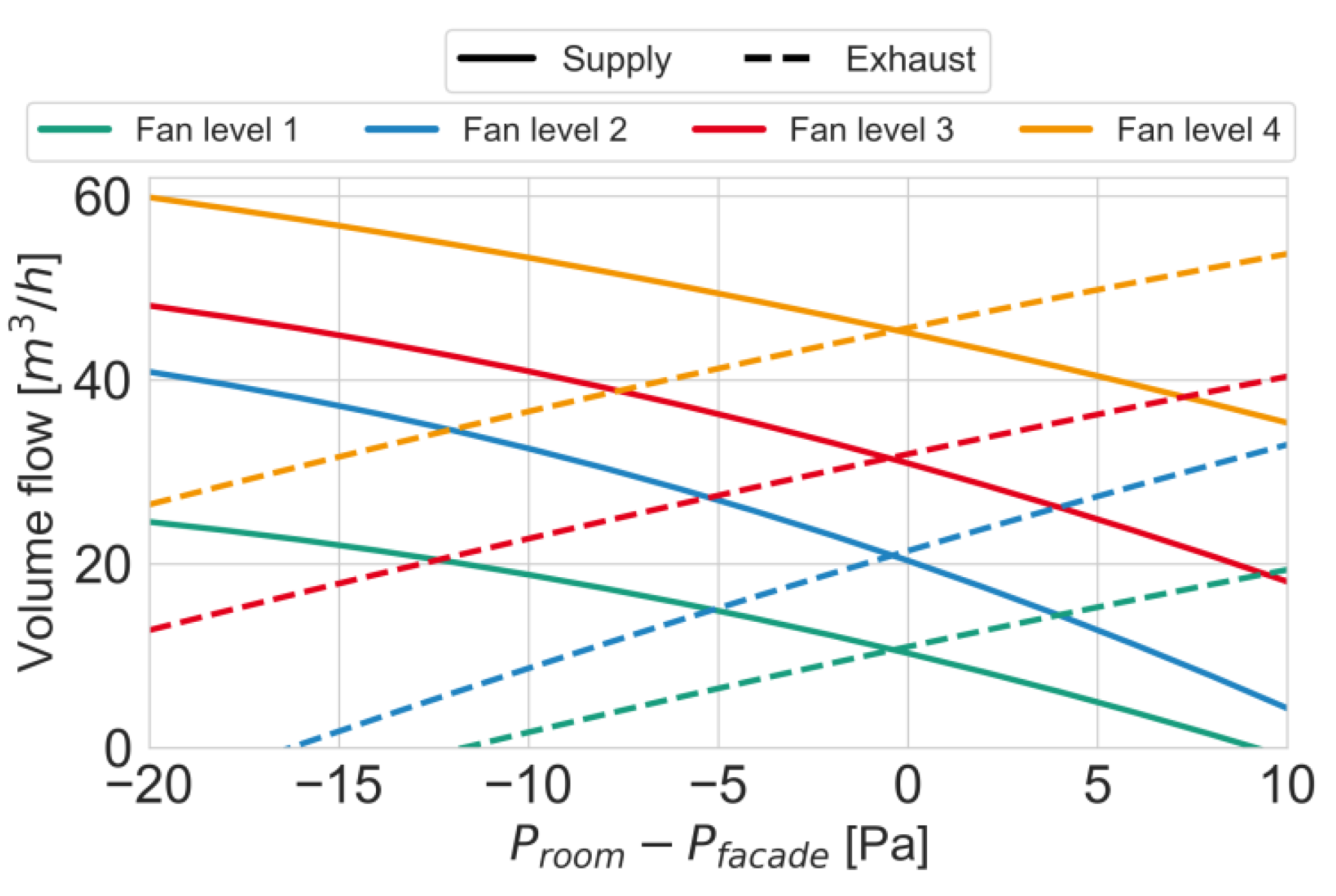
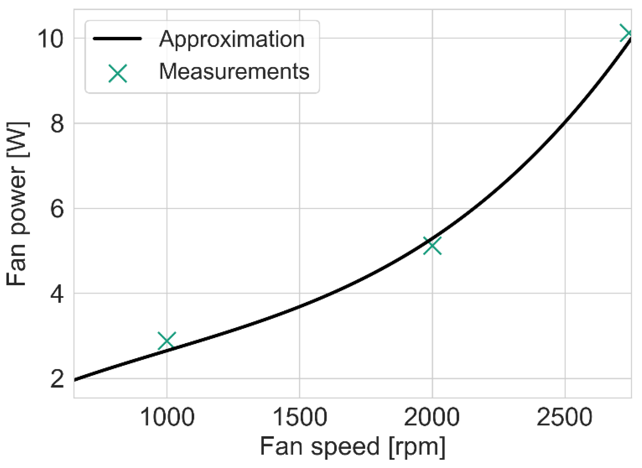
2.4. Fan Hydraulic Model
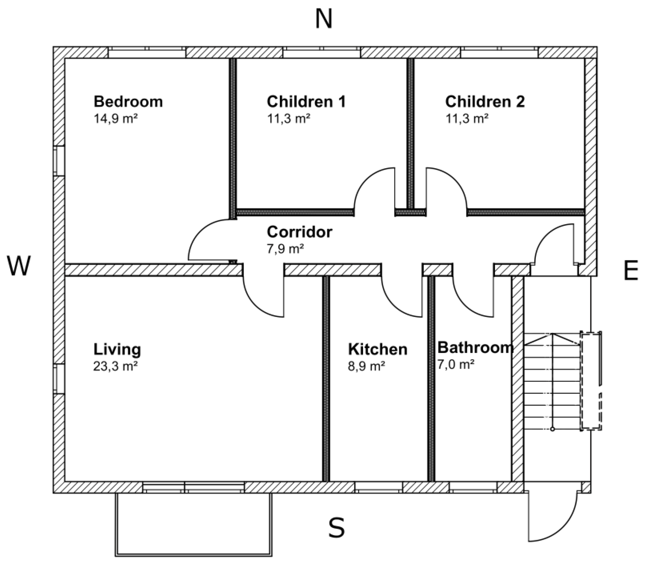
2.5. Building Model
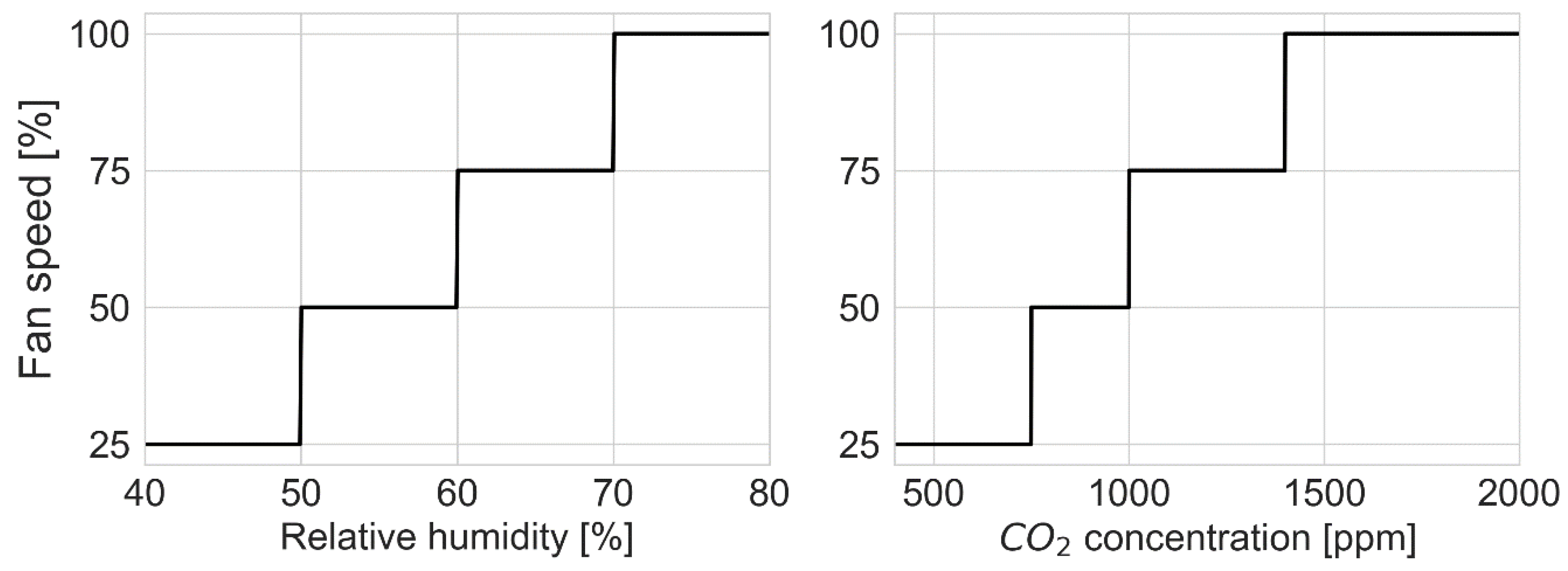
2.6. Performance Indicators
3. Heat Exchanger Model Validation
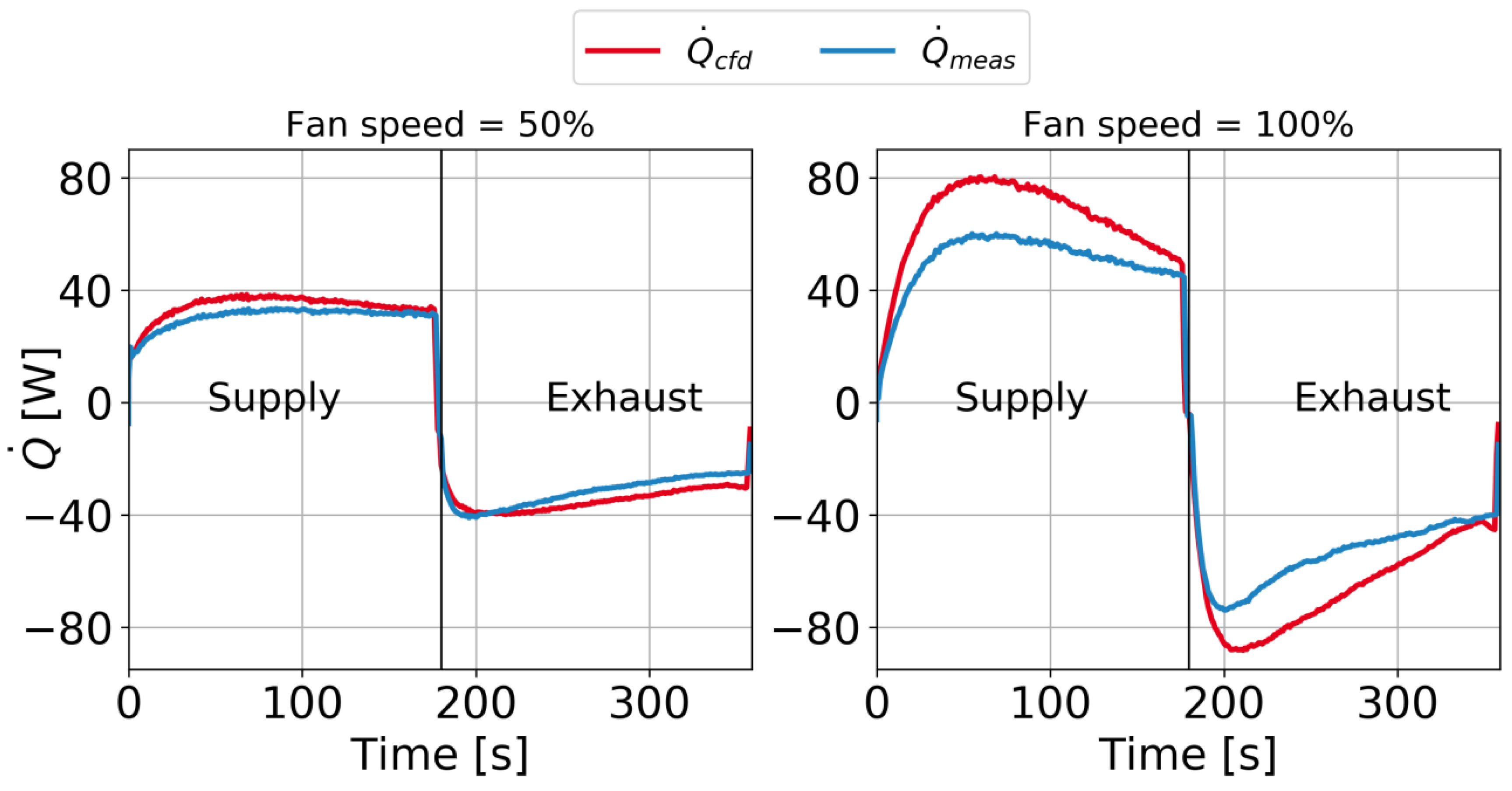
3.1. CFD
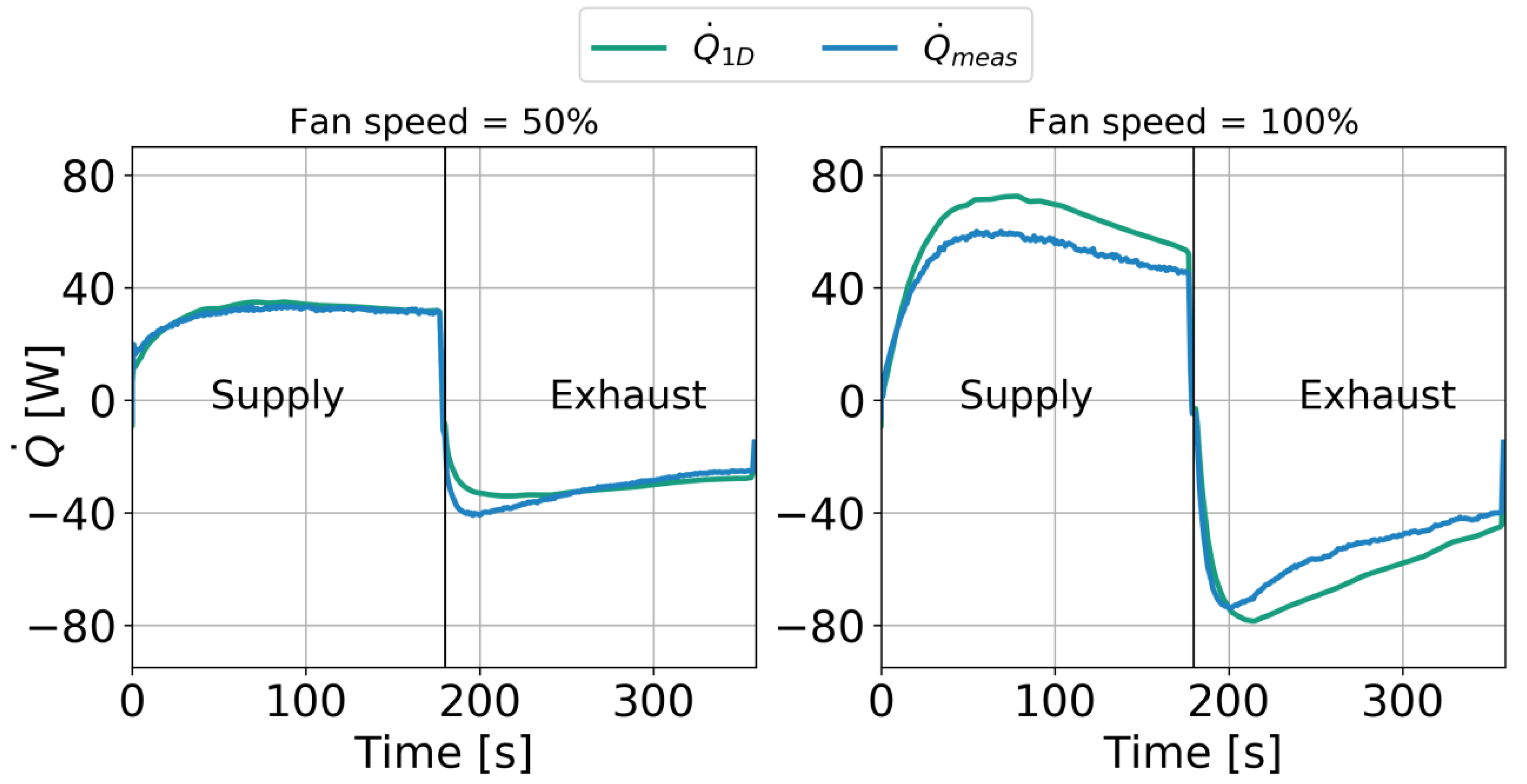
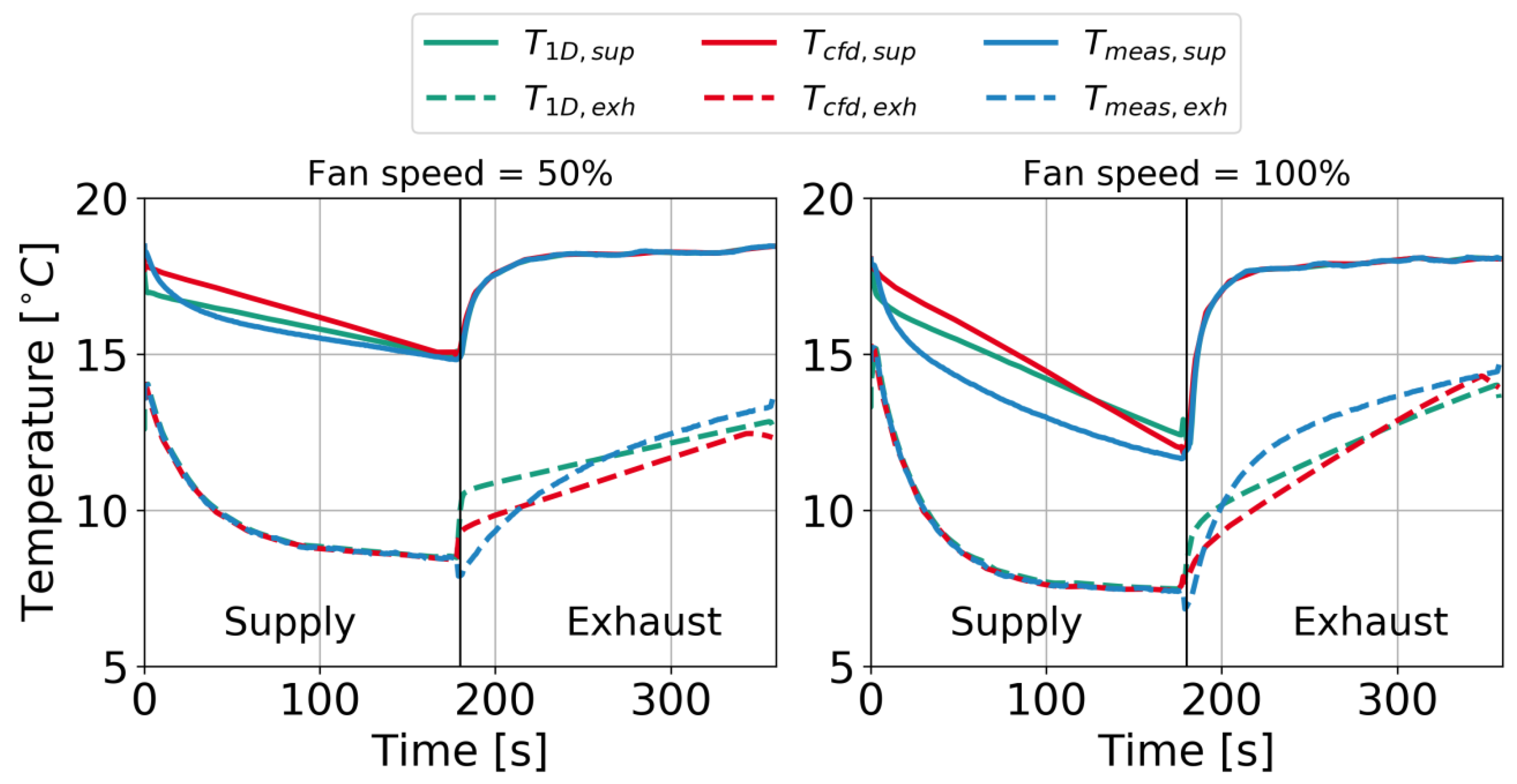
3.2. Modelica 1D Model
3.3. Comparison and Discussion
- Dynamic 1D mass and energy balance.
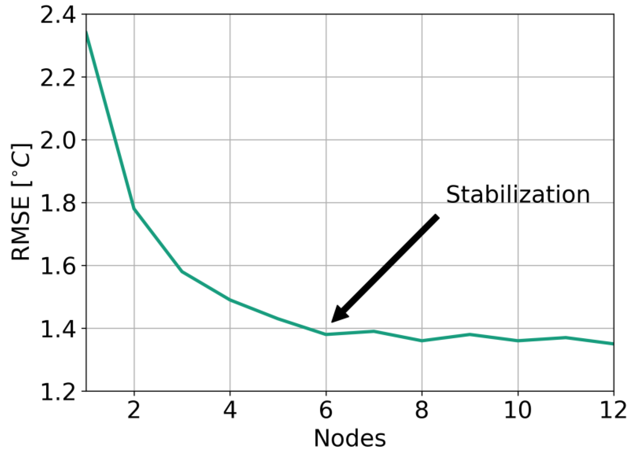
- Discretization in the axial direction (six nodes).
- Neglects radiation.
- Neglects thermal conductivity in heat storage.
- Neglects air velocity profile.
- The 1D model sufficiently calculates the experimentally evaluated behavior of the DRVS. Longer cycles and lower air velocities are better modeled compared to the measurements.
- CFD modeling could make sense for geometrical optimization but not for cycle evaluation.
- Measured heat recovery efficiencies are in a range between 54% and 80% accuracy. Higher air velocities and shorter cycles present higher efficiencies.
4. Case Study: Integrating DRVS into Building Simulation
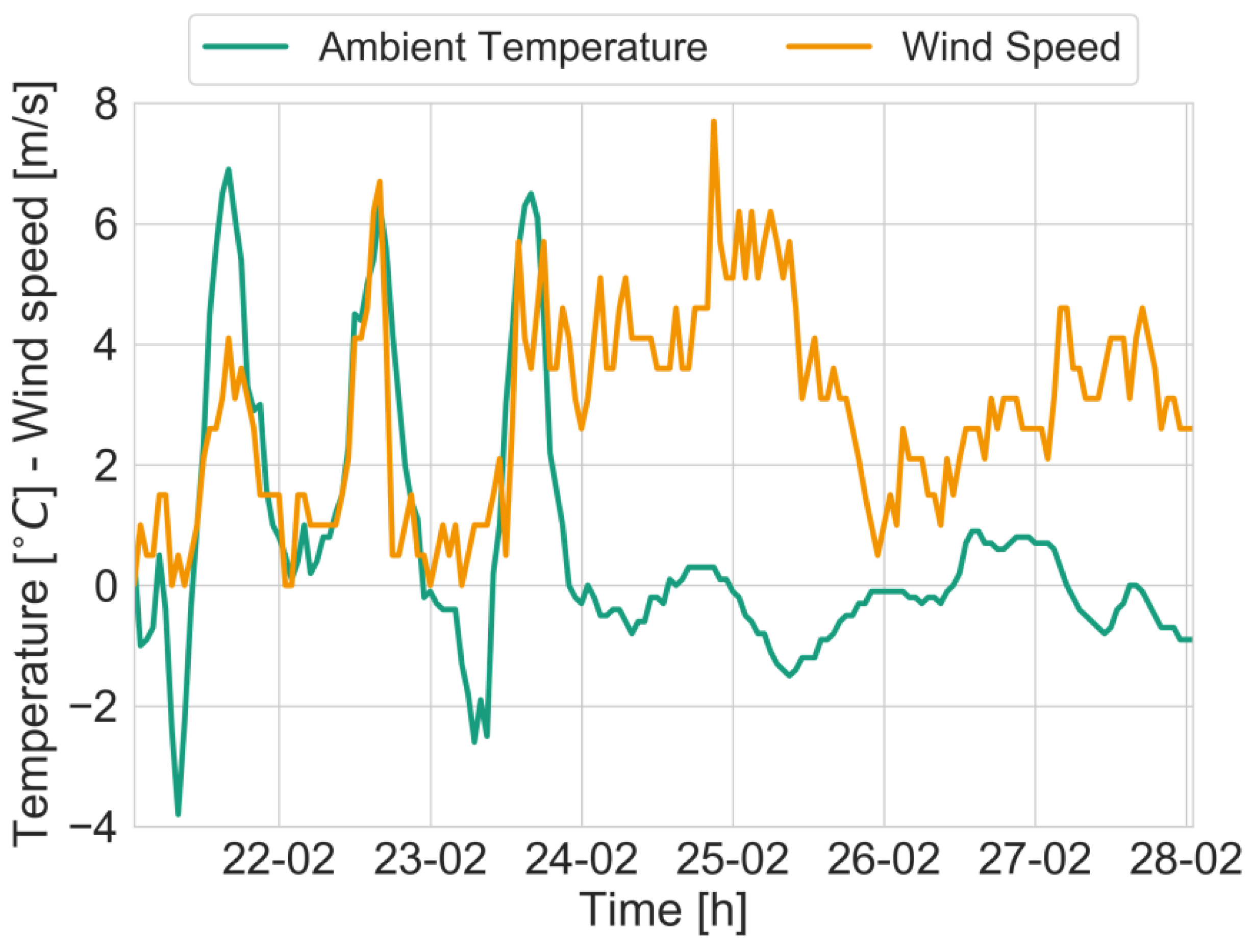
4.1. Simulation Set Up
- DRVS modeling including pressure difference with a component-based HRC model.
- DRVS modeling including pressure difference with a constant HRC efficiency of 70%.
- DRVS modeling neglecting pressure difference with a constant HRC efficiency of 70%.
4.2. Simulation Results
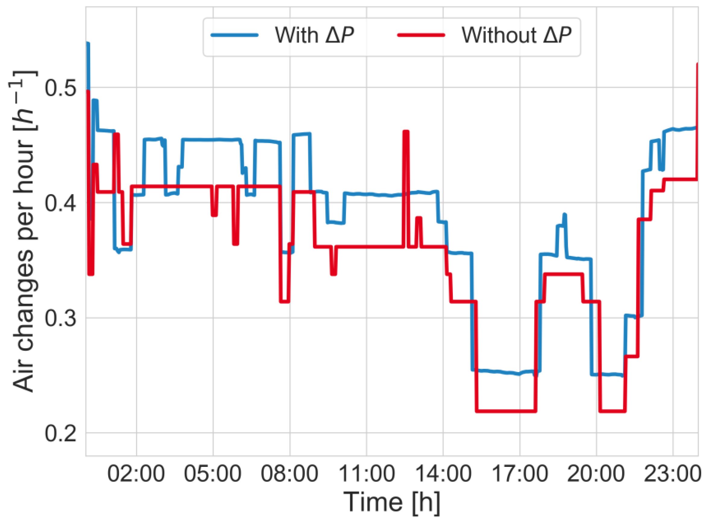
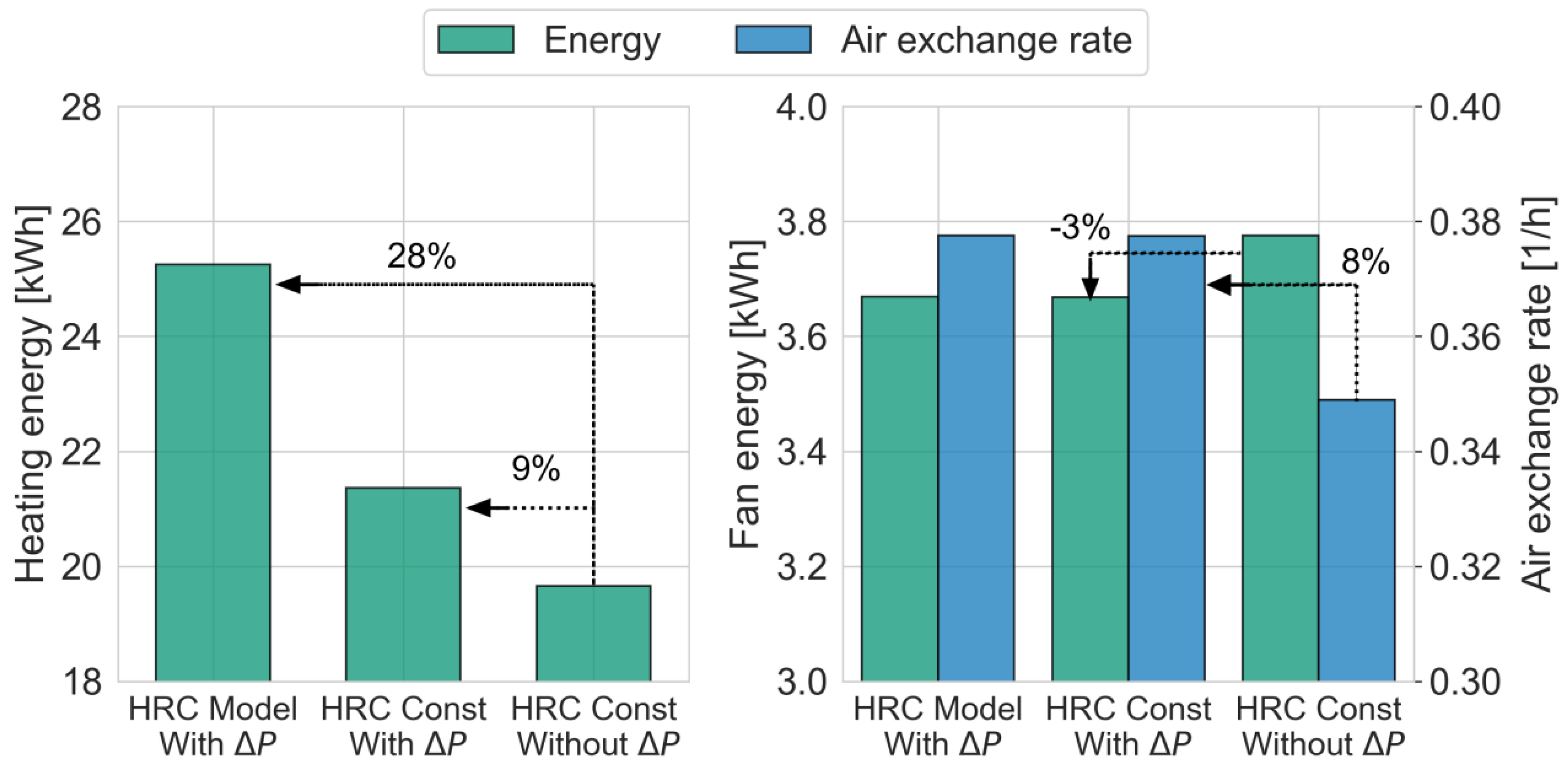
- Adding the pressure difference to the fan modeling results in an 8% higher air exchange rate, which causes 9% additional heat losses. Fan energy consumption is slightly lower (−3%), as the increasing volume flows reduce the fan speed on some occasions.
- Adding a component-based heat recovery system directly impacts the heat losses due to ventilation. Relative to the constant HRC case, it results in a 17% higher total heat losses, which means that the assumption of a global heat recovery efficiency leads to an underestimation of these losses in this simulation case.
- A component-based thermal and hydraulic model of DRVS results in a total of 28% higher heat losses due to ventilation. These results are not negligible in any case and should be included when integrating DRVSs in building performance simulation.
4.3. Discussion
5. Conclusions
Author Contributions
Funding
Conflicts of Interest
Nomenclature
| Variables | |
| Heat exchanged | |
| Heat transfer rate | |
| Pressure difference | |
| Volume flow | |
| Efficiency | |
| Power | |
| Temperature | |
| Time | |
| Mass flow | |
| specific heat coefficient | |
| Nu | Nusselt number |
| Re | Reynolds number |
| Pr | Prandtl number |
| Number of channels | |
| Channel width | |
| Channel length | |
| Density | |
| Thermal conductivity | |
| Wall thickness | |
| Area | |
| Specific convection coefficient | |
| Hydraulic diameter | |
| Subscripts | |
| meas | Measured |
| 1D | Simulated with 1D model |
| cfd | Simulated with CFD model |
| mean | Mean value |
| room | Room or indoor side |
| amb | Ambient or outdoor side |
| sup | Supply |
| exh | Exhaust |
| air | Air stream |
| solid | Regenerator |
| inf | Infiltrations |
| ht | Heat transfer |
| flow | Flowing |
| Abbreviations | |
| BDF | Backward differentiation formula |
| CFD | Computational fluid dynamics |
| DRVS | Decentralized regenerative ventilation system |
| DCV | Demand controlled ventilation |
| FEM | Finite elements method |
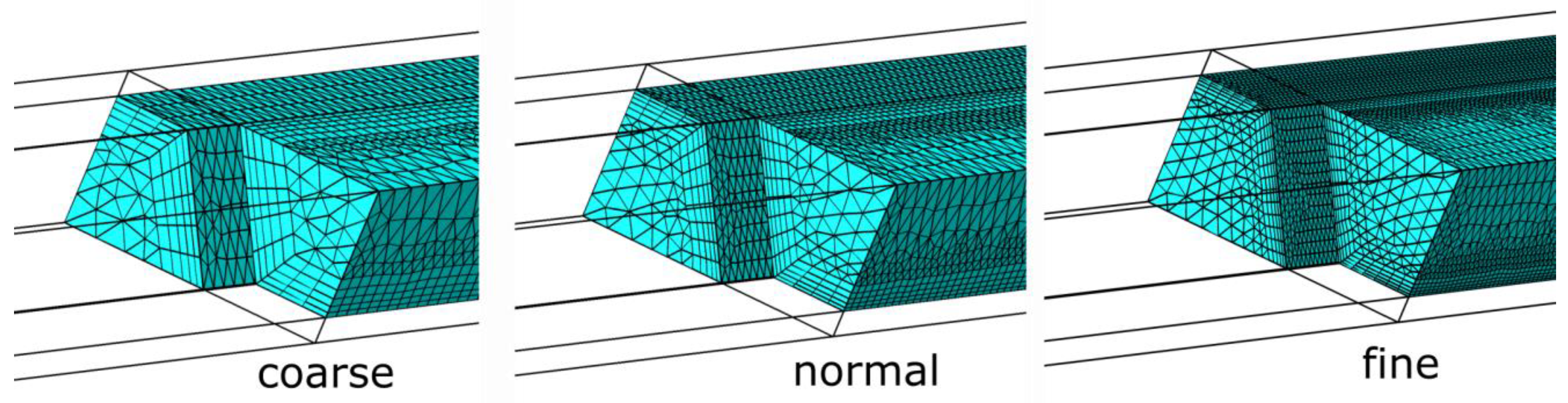
| GCI | Grid convergence indices |
| HRC | Heat recovery |
| MAPE | Mean absolute percentage error |
| RMSE | Root mean squared error |
References
- European Union Commision. Comprehensive Study of Building Energy Renovation Activities and the Uptake of Nearly Zero-Energy Buildings in the EU; European Commision: Brussels, Belgium, 2019; Available online: https://op.europa.eu/de/publication-detail/-/publication/97d6a4ca-5847-11ea-8b81-01aa75ed71a1 (accessed on 20 July 2020).
- Francisco, P.W.; Jacobs, D.E.; Targos, L.; Dixon, S.L.; Breysse, J.; Rose, W.; Cali, S. Ventilation, indoor air quality, and health in homes undergoing weatherization. Indoor Air 2017, 27, 463–477. [Google Scholar] [CrossRef] [PubMed]
- Interconnection Consulting. IC Market Tracking: Kontrollierte Wohnraumlüftung in Europa 2018; Interconnection Consulting: Oberstdorf, Germany, 2018; Available online: www.interconnectionconsulting.com (accessed on 14 October 2019).
- Viessmann GbmH. Dezentrales Wohnungslüftungsgerät Vitovent 100-D mit Wärmerückgewinnung. Available online: https://www.viessmann.de/de/wohngebaeude/wohnungslueftung/dezentrale-wohnungslueftung/vitovent-100-d.html (accessed on 20 July 2020).
- Angsten, R.; Hartmann, T. Raumweise Lüftungsgeräte in der Wohnungslüftung—Pro und contra. GI Wiss. 2017, 3, 210–215. [Google Scholar]
- Mikola, A.; Simson, R.; Kurnitski, J. The Impact of Air Pressure Conditions on the Performance of Single Room Ventilation Units in Multi-Story Buildings. Energies 2019, 12, 2633. [Google Scholar] [CrossRef]
- Baldini, L.; Goffin, P.; Leibundgut, H. Control strategies for effective use of wind loading through a decentralized ventilation system. In Proceedings of the ROOMVENT 2011-12th International Conference on Air Distribution in Rooms, Trondheim, Norway, 10–12 January 2021. [Google Scholar]
- Mahler, B.; Himmler, R. Results of the evaluation study DeAL Decentralized facade integrated ventilation systems. In Proceedings of the 8th International Conference for Enhanced Building Operations, Berlin, Germany, 20–22 October 2008; pp. 1–8. [Google Scholar]
- Merzkirch, A.; Maas, S.; Scholzen, F.; Waldmann, D. Field tests of centralized and decentralized ventilation units in residential buildings—Specific fan power, heat recovery efficiency, shortcuts and volume flow unbalances. Energy Build. 2016, 116, 376–383. [Google Scholar] [CrossRef]
- Coydon, F.; Herkel, S.; Kuber, T.; Pfafferott, J.; Himmelsbach, S. Energy performance of façade integrated decentralised ventilation systems. Energy Build. 2015, 107, 172–180. [Google Scholar] [CrossRef]
- Smith, K.; Svendsen, S. Control of Single-room Ventilation with Regenerative Heat Recovery for Indoor Climate and Energy Performance. In Proceedings of the CLIMA 2016—12th REHVA World Congress, Aalborg, Denmark, 22–25 May 2016. [Google Scholar]
- Manz, H.; Huber, H.; Schälin, A.; Weber, A.; Ferrazzini, M.; Studer, M. Performance of single room ventilation units with recuperative or regenerative heat recovery. Energy Build. 2000, 31, 37–47. [Google Scholar] [CrossRef]
- Mathis, P.; Röder, T.; Hartmann, T.; Knaus, C.; Klein, B.; Müller, D. Ventilation efficiency of decentralized alternating residential ventilation unit. REHVA J. 2019, 4, 8–12. [Google Scholar]
- Muralikrishna, S. Study of Heat Transfer Process in a Regenerator. Chem. Eng. Res. Des. 1999, 77, 131–137. [Google Scholar] [CrossRef]
- Liu, H.; Yu, Q.N.; Zhang, Z.C.; Qu, Z.G.; Wang, C.Z. Two-equation method for heat transfer efficiency in metal honeycombs: An analytical solution. Int. J. Heat Mass Transf. 2016, 97, 201–210. [Google Scholar] [CrossRef]
- Mesonero, I.; Febres, J.; López Pérez, S. Modeling and simulation of fixed bed regenerators for a multi-tower decoupled advanced solar combined cycle. In Proceedings of the 12th International Modelica Conference, Prague, Czech Republic, 15–17 May 2017; pp. 847–855. [Google Scholar] [CrossRef]
- Gateau, P.; Namy, P.; Huc, N. Comparison between Honeycomb and Fin Heat Exchangers. In Proceedings of the Comsol Conference. 2011. Available online: https://www.tib.eu/en/search/id/TIBKAT%3A689211589/ (accessed on 31 December 2012).
- Li, Q.; Wang, Z.; Bai, F.; Chu, S.; Yang, B. Thermal Analysis of Honeycomb Ceramic Air Receiver. In AIP Conferece Proccedings 1850; AIP Publishing LLC: Melville, NY, USA, 2017; Volume 160016. [Google Scholar] [CrossRef]
- Auerswald, S.; Pflug, T.; Engelmann, P.; Carbonare, N.; Bongs, C.; Dinkel, A.; Henning, H.-M. A holistic evaluation method for decentralized ventilation systems. In Proceedings of the 39th AIVC Conference, Antibes Juan-Les-Pins, France, 18–19 September 2018. [Google Scholar]
- Ljubijankic, M.; Nytsch-Geusen, C.; Rädler, J.; Löffler, M. Numerical coupling of Modelica and CFD for building energy supply systems. In Proceedings of the 8th Modelica Conference, Dresden, Germany, 20–22 March 2011; pp. 286–294. [Google Scholar]
- Asadov, N. Simulation and Measurement of Different Geometries and Materials for Heat Exchangers in Decentralized Regenerative Ventilation Devices. Master’s Thesis, Fraunhofer ISE, Universität Freiburg, Freiburg im Breisgau, Germany, 2019. [Google Scholar]
- Celik, I.B.; Ghia, U.; Roache, P.J.; Freitas, C.J.; Coleman, H.; Raad, P.E. Procedure for Estimation and Reporting of Uncertainty Due to Discretization in CFD Applications. J. Fluids Eng. 2008, 130. [Google Scholar] [CrossRef]
- Li, Q.; Bai, F.; Yang, B.; Wang, Z.; El Hefni, B.; Liu, S.; Kubo, S.; Kiriki, H.; Han, M. Dynamic simulation and experimental validation of an open air receiver and a thermal energy storage system for solar thermal power plant. Appl. Energy 2016, 178, 281–293. [Google Scholar] [CrossRef]
- Shah, R.K.; Sekulić, D.P. Fundamentals of Heat Exchanger Design; John Wiley & Sons: Hoboken, NJ, USA, 2003; ISBN 0471321710. [Google Scholar]
- Mattsson, S.E.; Elmqvist, H. Modelica—An international effort to design the next generation modeling language. In Proceedings of the 7th IFAC Symposium on Computer Aided Control Systems Design, Gent, Belgium, 28–30 April 1997; pp. 1–5. [Google Scholar]
- Wetter, M.; Zuo, W.; Nouidui, T.S.; Pang, X. Modelica Buildings library. J. Build. Perform. Simul. 2014, 7, 253–270. [Google Scholar] [CrossRef]
- Deutsches Institut für Bautechnik. Zulassungsbericht Z-51.3-415: Dezentrales Wohnungslueftungsgeraet mit Waermerueckgewinnung vom Typ Vitovent 100-D H00E A45; DIBt: Berlin, Germany, 2019. [Google Scholar]
- Ebert, B. LowEx-Bestand Analyse Abschlussbericht zu AP 1.1. Systematische Analyse von Mehrfamilien-Bestandsgebäuden. 2018. Available online: https://www.lowex-bestand.de/index.php/downloads/?lang=de&download=77 (accessed on 20 March 2019).
- Crawley, D.B.; Lawrie, L.K.; Winkelmann, F.C.; Buhl, W.F.; Huang, Y.J.; Pedersen, C.O.; Strand, R.K.; Liesen, R.J.; Fisher, D.E.; Witte, M.J.; et al. EnergyPlus: Creating a new-generation building energy simulation program. Energy Build. 2001, 33, 319–331. [Google Scholar] [CrossRef]
- Boyer, H.; Lauret, A.P.; Adelard, L.; Mara, T.A. Building ventilation: A pressure airflow model computer generation and elements of validation. Energy Build. 1999, 29, 283–292. [Google Scholar] [CrossRef]
- Swami, M.V.; Chandra, S. Procedures for Calculating Natural Ventilation Airflow Rates in Buildings; ASHRAE Research PRoject 448-RP No. 1; Florida Solar Energy Center: Cocoa, FL, USA, 1987. [Google Scholar]
- Orme, M.; Liddament, M.W.; Wilson, A. Numerical Data for Air Infiltration & Natural Ventilation Calculation; Energy Conservation in buildings and Community Systems Program; AIVC: Coventry, UK, February 1998. [Google Scholar]
- International Organization for Standardization. ISO 18523-2:2018—Energy Performance of Buildings—Schedule and Condition of Building—Zone and Space Usage for Energy Calculation. Part 2: Residential Buildings, 1st ed.; ISO: Geneva, Switzerland, 2018. [Google Scholar]
- Ahmed, K.; Kurnitski, J.; Olesen, B. Data for occupancy internal heat gain calculation in main building categories. Data Brief 2017, 15, 1030–1034. [Google Scholar] [CrossRef]
- Firlag, S.; Zawada, B. Impacts of airflows, internal heat and moisture gains on accuracy of modeling energy consumption and indoor parameters in passive building. Energy Build. 2013, 64, 372–383. [Google Scholar] [CrossRef]
- TenWolde, A.; Pilon, C.L. The Effect of Indoor Humidity on Water Vapor Release in Homes. In Proceedings Thermal Performance of the Exterior Envelopes of 2007; Building: Clearwater, FL, USA, 2007. [Google Scholar]
- Persily, A.; de Jonge, L. Carbon dioxide generation rates for building occupants. Indoor Air 2017, 27, 868–879. [Google Scholar] [CrossRef]
- Schweiker, M.; Haldi, F.; Shukuya, M.; Robinson, D. Verification of stochastic models of window opening behaviour for residential buildings. J. Build. Perform. Simul. 2012, 5, 55–74. [Google Scholar] [CrossRef]
- Deutsches Institut für Normung e.V. DIN 1946-6-Raumlufttechnik- Teil 6-Lüftung von Wohnungen—Allgemeine Anforderungen, Anforderungen an die Auslegung, Ausführung, Inbetriebnahme und Übergabe sowie Instandhaltung, 1st ed.; Beuth Verlag GmbH: Berlin, Germany, 2019. [Google Scholar]
- Carbonare, N.; Pflug, T.; Bongs, C.; Wagner, A. Comfort-oriented control strategies for decentralized ventilation using co-simulation. IOP Conf. Ser. Mater. Sci. Eng. 2019, 609, 1–6. [Google Scholar] [CrossRef]
- Carbonare, N.; Pflug, T.; Bongs, C.; Wagner, A. Simulation study of a novel fuzzy demand controlled ventilation for façade-integrated decentralized systems. Sci. Technol. Built Environ. 2020, 26, 1412–1426. [Google Scholar] [CrossRef]
- Deutsches Institut für Normung e.V.; European Committee for Standardization. DIN EN 308. Wärmeaustauscher—Prüfverfahren zur Bestimmung der Leistungskriterien von Luft/Luft und Luft/Abgas-Wärmerückgewinnungsanlagen; Beuth Verlag GmbH: Berlin, Germany, 1997. [Google Scholar]
- Armstrong, J.S.; Collopy, F. Error measures for generalizing about forecasting methods: Empirical comparisons. Int. J. Forecast. 1992, 8, 69–80. [Google Scholar] [CrossRef]
- Zemitis, J.; Bogdanovics, R. Heat recovery efficiency of local decentralized ventilation device at various pressure differences. Mag. Civil Eng. 2020, 94, 120–128. [Google Scholar] [CrossRef]
- Krajčík, M.; Simone, A.; Olesen, B.W. Air distribution and ventilation effectiveness in an occupied room heated by warm air. Energy Build. 2012, 55, 94–101. [Google Scholar] [CrossRef]
- Merzkirch, A. Energieeffizienz, Nutzerkomfort und Kostenanalyse von Lüftungsanlagen in Wohngebäuden: Feldtests von neuen Anlagen und Vorstellung bedarfsgeführter Prototypen. Ph.D. Thesis, Université du Luxembourg, Luxembourg, 2015. [Google Scholar]
- Pastore, L.; Andersen, M. Building energy certification versus user satisfaction with the indoor environment: Findings from a multi-site post-occupancy evaluation (POE) in Switzerland. Build. Environ. 2019, 150, 60–74. [Google Scholar] [CrossRef]


| Variable | Unit | Value |
|---|---|---|
| Channel width w | m | 0.004 |
| Channel length l | m | 0.15 |
| Channel area | m2 | 4.16 × 10⁻⁵ |
| Cylinder diameter d | m | 0.142 |
| Free flow area | m2 | 0.0104 |
| Mass | kg | 2.32 |
| Specific heat capacity | J kg−1 K−1 | 877 |
| Density | kg m−3 | 2700 |
| Thermal conductivity | W m−1 K−1 | 0.026 |
| Number of channels | - | 1000 |
| Wall thickness | m | 0.001 |
| Cycle Length | Fan Speed | ||
|---|---|---|---|
| 60 s | 50% | 0.40 | 92 |
| 100% | 0.89 | 204 | |
| 180 s | 50% | 0.40 | 92 |
| 100% | 0.89 | 204 |
| Sensor | Model | Range | Accuracy | Response Time |
|---|---|---|---|---|
| Temperature | IST RTD Platinum | −50–+150 °C | ±0.1 K (after calibration) | = 1200 ms ( =1 m/s) |
| Humidity | Vaisala HMT 120 | 0–100% rH | ±1.5% rH | |
| Differential pressure | h-w PU ± 50 | −50–+50 Pa | ±0.5% m.v. | 20 ms |
| Mass flow rate | E+H B200 Prosonic Flow | 0–300 m3.h1 | ±1.5% m.v. | = 1000 ms |
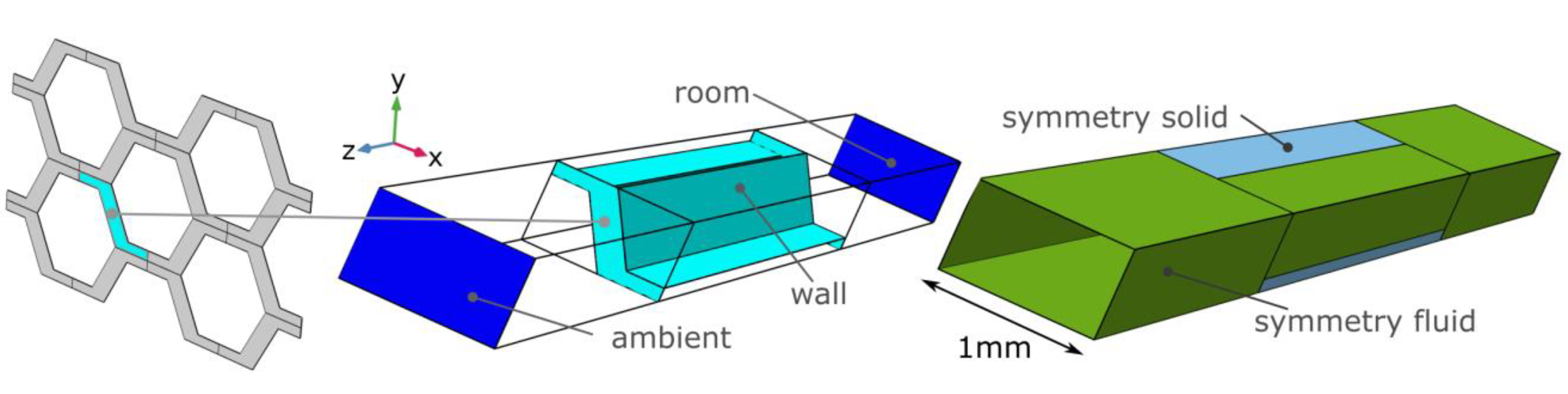
| Boundary | and Pressure | Comment | |
|---|---|---|---|
| Ambient face | Supply phase: exhaust phase: | Supply phase: exhaust phase: | |
| Room face | Supply phase: exhaust phase: | , (abs. pressure) Tangential stress component is set to zero | |
| Symmetry fluid | No penetration and vanishing shear stresses | ||
| Symmetry solid | – | – | |
| Wall | – | No slip condition |
| Child 2 | Child 1 | Bedroom | Living | Kitchen | Bathroom |
|---|---|---|---|---|---|
| 20(16) | 20(16) | 20(16) | 20 | 20 | 22 |
| Period [s] | 60 s | 180 s | ||
|---|---|---|---|---|
| Variable | ||||
| 50% Speed | 0.83 | 30.7 | 0.80 | 33.4 |
| 100% Speed | 0.75 | 54.5 | 0.66 | 63.4 |
| Period (s) | 60 s | 180 s | ||||||
|---|---|---|---|---|---|---|---|---|
| Variable | ||||||||
| 50% Speed | 0.77 | 0.80 | 25.3 | 27.0 | 0.76 | 0.75 | 30.6 | 29.9 |
| 100% Speed | 0.71 | 0.64 | 47.6 | 40.0 | 0.63 | 0.54 | 59.0 | 49.1 |
| Model | Period (s) | 60 s | 180 s | Simulation Time | ||
|---|---|---|---|---|---|---|
| RMSE (°C) | MAPE (%) | RMSE (°C) | MAPE (%) | |||
| CFD | 50% | 0.8 | 4.5 | 0.6 | 3.6 | >8 h |
| 100% | 1.5 | 9.6 | 1.3 | 9.1 | ||
| 1D Model (Modelica) | 50% | 0.6 | 2.3 | 0.3 | 1.6 | 0.17 s |
| 100% | 1.1 | 6.9 | 1.1 | 7.6 | ||
Publisher’s Note: MDPI stays neutral with regard to jurisdictional claims in published maps and institutional affiliations. |
© 2020 by the authors. Licensee MDPI, Basel, Switzerland. This article is an open access article distributed under the terms and conditions of the Creative Commons Attribution (CC BY) license (http://creativecommons.org/licenses/by/4.0/).
Share and Cite
Carbonare, N.; Fugmann, H.; Asadov, N.; Pflug, T.; Schnabel, L.; Bongs, C. Simulation and Measurement of Energetic Performance in Decentralized Regenerative Ventilation Systems. Energies 2020, 13, 6010. https://doi.org/10.3390/en13226010
Carbonare N, Fugmann H, Asadov N, Pflug T, Schnabel L, Bongs C. Simulation and Measurement of Energetic Performance in Decentralized Regenerative Ventilation Systems. Energies. 2020; 13(22):6010. https://doi.org/10.3390/en13226010
Chicago/Turabian StyleCarbonare, Nicolas, Hannes Fugmann, Nasir Asadov, Thibault Pflug, Lena Schnabel, and Constanze Bongs. 2020. "Simulation and Measurement of Energetic Performance in Decentralized Regenerative Ventilation Systems" Energies 13, no. 22: 6010. https://doi.org/10.3390/en13226010
APA StyleCarbonare, N., Fugmann, H., Asadov, N., Pflug, T., Schnabel, L., & Bongs, C. (2020). Simulation and Measurement of Energetic Performance in Decentralized Regenerative Ventilation Systems. Energies, 13(22), 6010. https://doi.org/10.3390/en13226010