Abstract
Thermal energy is an important input of furniture components production. A thermal energy production system includes complex, non-linear, and changing combustion processes. The main focus of this article is the maximization of thermal energy production considering the inbuilt complexity of the thermal energy production system in a factory producing furniture components. To achieve this target, a data-driven prediction and optimization model to analyze and improve the performance of a thermal energy production system is implemented. The prediction models are constructed with daily data by using supervised machine learning algorithms. Importance analysis is also applied to select a subset of variables for the prediction models. The modeling accuracy of prediction algorithms is measured with statistical indicators. The most accurate prediction result was obtained using an artificial neural network model for thermal energy production. The integrated prediction and optimization model is designed with artificial neural network and particle swarm optimization models. Both controllable and uncontrollable variables were used as the inputs of the maximization model of thermal energy production. Thermal energy production is increased by 4.24% with respect to the optimal values of controllable variables determined by the integrated optimization model.
1. Introduction
The world’s fossil fuel reserves have gradually been depleted with the growth in industry, transportation, population, and urban areas. Accordingly, the environmental impacts of high fossil fuel consumption have also increased considerably. Biomass is a suitable renewable energy resource that can substitute for fossil fuels to restrain greenhouse gas emissions [1,2,3]. Biomass resources can be converted to a more useful energy form with thermal processes called combustion, gasification, and pyrolysis [4]. Combustion is the burning of biomass in the air to produce hot gases and ash. Then, stored chemical energy is converted into heat, which is transformed to kinetic energy through heating water to produce vapor used for gas engines [5]. Great diversity in biomass resources creates the need for adaptable combustion technology in order to achieve efficient and clean biomass combustion [6]. Grate-fired boilers are the leading technologies in biomass combustion for heat and power production. They can fire different types of fuels with variable moisture levels using efficient fuel preparation and less handling effort [1,7]. The stability of thermal energy production (TEP) can be maintained by closely monitoring and controlling the grate-firing process. Current control technologies of the grate-firing process still need improvement to enhance system efficiency, emission control, and operational automation [8]. Mathematical and computational fluid dynamics (CFD) models provide useful tools for the simulation, optimization and control of grate-fired boilers [1,9,10,11]. However, the grate-firing process consists of complex operations with chemical and physical reactions. Developing analytical models of the grate-firing process is challenging because of its inherent complexity [12,13]. Data-driven methods offer an alternative way to tackle complex and non-linear problems.
In engineering studies, data are represented as attribute-value pairs with corresponding measurement units. When the experimental data of any industrial application are attained, hidden engineering knowledge in the dataset can be extracted with predictive models. Data-driven methods are promising approaches for modeling and optimization, and they have been applied in various industries such as production systems, healthcare, energy, pollution, emission control, and supply chains [14,15,16,17,18,19,20]. Kusiak and Smith (2007) [14] outlined the usefulness of data-mining algorithms for extracting knowledge from a large volume of data, leading to significant improvements in the next generation of products and services. Mishra et al. (2020) [15] presented an enhanced and adaptive genetic algorithm model used with a multilayer perceptron neural network (MLPNN) to detect the presence of diabetes in patients to assist medical experts. Sun et al. (2019) [16] used a backpropagation artificial neural network (ANN)-based extreme learning machine to estimate the remaining useful life of lithium-ion batteries. Rushdi et al. (2020) [17] employed machine learning regression methods to predict the power generated by airborne wind energy systems. Yoo et al. (2016) [18] proposed an integrated ordinal pairwise partitioning and decision tree approach to estimate patterns of groundwater pollution sensitivity with improved accuracy and consistency. Mihaita et al. (2019) [19] applied machine learning modeling using decision trees and ANNs and showed that humidity and noise were the most important factors influencing the prediction of nitrogen dioxide concentrations of mobile stations. Chen et al. (2019) [20] developed an inventory model considering the revenue of an online pharmacy and waste of resources caused by excessive inventory for online pharmacies green supply chain management. They used a genetic algorithm (GA)-based solution procedure to determine the optimal product image location, product price, and procurement quantity to maximize profit.
Modeling and simulation efforts in relation to biomass combustion and heat transfer in grate-fired boilers, oil heaters with convection and radiation systems, heat exchangers, etc. continue to be a research subject [1]. Predictive models play an important role in the management of renewable energy systems. The grate-firing process can be modeled by using data-driven methods to perform generalization at high speed with the availability of historical data in database- management systems. Data-mining algorithms are popular methods for this, and there are a couple of articles in the literature related to building data mining prediction models for industrial boilers using fossil and biomass fuels as energy resources [21,22,23,24,25,26,27,28,29,30,31,32]. A review of the application of artificial intelligence in modeling and prediction of the performance and control of the combustion process is given by Kalogirou (2003) [21]. Chu et al. (2003) [22] proposed a constrained optimization procedure using ANNs as the modeling tool for the emission control and thermal efficiency of combustion in a coal-fired boiler. Hao et al. (2003) [23] illustrated the ability of ANNs to model complex coal combustion performance in a tangentially fired boiler. They stated that ANNs may not have directly provided a better understanding of the complex combustion processes in boilers than the CFD method, but ANNs were alternative approaches for the engineers to evaluate the combustion performance of the boilers with easier application and shorter computation time than the CFD method. Rusinowski and Stanek (2007) [24] presented the back-propagation neural modeling of coal-fired steam boilers. Their model described the dependence of the operational parameters upon the flue gas losses and losses due to unburned combustibles. Chandok et al. (2008) [25] presented a radial basis function and back-propagation neural network approaches to estimate furnace exit gas temperature of pulverized coal-fired boiler for operator information. A least-squares support vector machine approach was proposed by Gu et al. (2011) [26] to track the time-varying characteristics of a boiler combustion system to improve the energy efficiency and reduce pollutants emissions of power units. Liukkonen et al. (2011) [27] provided a useful approach by combining self-organizing maps, k-means clustering, and ANNs for monitoring the combustion process to increase its efficiency and reduce harmful emissions in a circulating fluidized bed boiler. Lv et al. (2013) [28] designed an ensemble method including a fuzzy c-means clustering algorithm, least-square support vector machine, and partial least square approaches to predict emission of coal-fired boiler. A black-box model for the prediction of fuel-ash-induced agglomeration of the bed materials in fluidized bed combustion was created through multivariate regression modeling by Gatternig and Karl (2015) [29]. Toth et al. (2017) [30] used image-based deep neural networks to predict the thermal output of a 3 MW step-grate biomass boiler. Böhler et al. (2019) [31] presented models for the prediction of emissions based on the measured flue gas oxygen concentration and combustion temperature in a small-scale biomass combustion furnace for wooden pellets. Fuzzy black-box models provided the most promising prediction results. Yang et al. (2020) [32] employed the least-squares support vector machine method as a real time dynamic prediction model of emission of a coal-fired boiler.
Optimization models of boiler systems are studied using evolutionary algorithms, swarm intelligence algorithms, etc. in the literature. Hao et al. (2001) [33] obtained optimal combustion parameters of pulverized coal-fired utility boiler by using combined ANN and GA. Hao et al. (2003) [23] suggested ANN and GAs as effective methods to model the carbon burnout behavior and to optimize the operational conditions in a tangentially fired utility boiler. Si et al. (2009) [34] proposed an integrated optimization approach based on a non-dominated sorting genetic algorithm-II for the optimal operation of a coal-fired boiler. Zhou et al. (2012) [35] modeled emissions from coal-fired utility boilers by using support vector regression (SVR) with an ant colony optimization algorithm. Wang et al. (2018) [36] applied a Gaussian process to model the relationship between emission and boiler operation by using GA for the optimization of the hyperparameters of the Gaussian process model. Shi et al. (2019) [37] developed an optimization method utilizing GA based on ANN in a coal-fired boiler to optimize the air distribution scheme for higher thermal efficiency and lower emission. In this article, supervised machine learning (SML) algorithms are used to predict TEP from operational data. The thermal energy production system (TEPS) is composed of a grate-fired boiler, an oil heater with convection and radiation zones, heat exchangers, and a steam generator [1,25] in a factory producing furniture components and includes complex processes. Regression tree (RT), random forest (RF), non-linear regression (NLR), SVR, and ANN are the SML methods used to create data-driven prediction models of TEP with rather low computational complexity and short computation times. Five different SML algorithms are theoretically explained with formulations. Afterwards, proposed SML methods are employed to build the prediction model of TEP. The convenient decision variables are chosen with tree-based algorithms to reduce the dimensionality of the inputs. Using the test data, the prediction accuracy of the models is evaluated with five different statistical indicators. Moreover, an integrated prediction and optimization model of TEPS is designed. An integrated model is used to maximize the objective function depending on controllable and uncontrollable decision variables. The optimal values of controllable variables for daily observations are researched with ANN simulation connected with particle swarm optimization (PSO) to maximize TEP for each day, while the values of uncontrollable variables are taken exactly as their observed values in the optimization model. To the best of the authors’ knowledge, both SML algorithms for the TEP prediction and the integrated ANN–PSO model for the maximization of TEP in a factory producing furniture components are implemented and applied for the first time in the literature in this article.
The remainder of this article is organized as follows. In the next section, RT, RF, NLR, SVR, ANN, and PSO models and their application at a factory producing furniture components are explained. In Section 3, the obtained results are presented and discussed. Finally, Section 4 gives the conclusion and future research objectives.
2. Methodology
2.1. The Facility
In this article, the proposed data-driven approaches are applied to a private company serving the furniture components industry in Turkey and international markets. The company’s product range includes wood-based composite panels, such as high-density fiberboard (HDF), medium-density fiberboard (MDF), and laminated MDF [38], and other wood products, such as wood and parquet floorings, wooden profiles, wooden doors, etc., produced from wood-based composite panels. The wood-based panel production line in the factory involves debarkers, chippers, chips storage yard, screening machines, washer, synthetic adhesive production unit, refiner, dryer, cyclones, fiber sifter, mat former, precompressor, continuous press, saws, cooler, stacking station, sander and cut-to-size machines, and a supervisory control and data acquisition (SCADA) system. The SCADA system collects instantaneous signals from sensors, constitutes a database, and is used as a control interface. The fully automated production line for wood-based panels is connected with the TEPS. The flow chart of the fiberboard production line in the factory is presented in Figure 1.
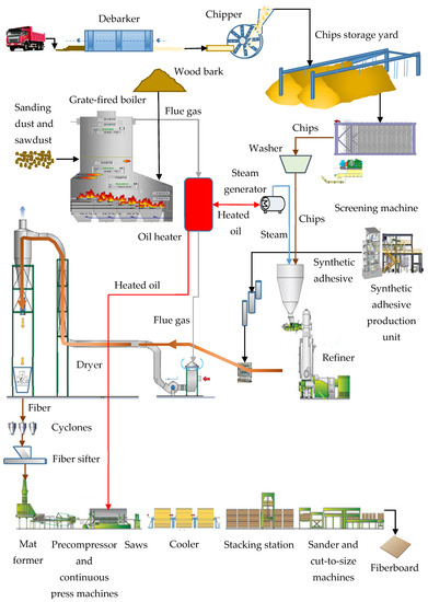
Figure 1.
The flow chart of the fiberboard production line.
The quality of wood-based panels mostly depends on the proper production of chips and fiber. The chips are attained from pine and beech wood using chipper machines. Chips are temporarily held in the chips storage yard prior to the screening process, which ensures the cleanliness and uniformity of wood chips. Then, chips are transferred into a washer to separate from foreign materials. The washing process helps to improve the performance of the refining system. Dewatered chips are moved to a pressurized refiner chamber for fiber production with a refining process. After resin, wax, and other additives are blended with the fibers inside the blow line, fibers are pneumatically conveyed through the dryer duct and dried to the required moisture content. Fiber cyclones separate the fibers from the flue gas stream. Fibers are discharged by airlocks and fed into the fiber sifter before the mat-forming process in the wood-based panel production line. The dried fibers are passed through a sifter to separate dense resin particles and defects from the fibers. Dried and resin-coated fibers are laid down on the mat former before they are sent to the precompressor and hot-press machine. The process of pressing is another crucial factor influencing the quality of the wood-based panels. The main influencers of the process of pressing are temperature and pressure. Oil, distributed from the oil collector and circulated in the system, is steered through the convection and the radiation zones of the oil heater to be heated with the flue gas. The oil heater operates as a single-pass system. The oil is directed into the inlet headers, and flows through the curved coils on the convection zone. Afterwards, it passes through the heat exchangers in the radiation zone. Then, heated oil is obtained to transfer heat to the hot press, melamine press, and impregnation machines at the same time. Melamine press and impregnation machines are located in a separate production line and are especially used for the production of laminated MDF products. The fiberboards are cut, sized, and sanded after the cooling process. The targeted thickness and surface smoothness of the wood-based panels are obtained with a sanding process.
The grate-fired boiler is one of the leading technologies used in biomass combustion, and released flue gas with the combustion of biomass is used for TEP. The design of the grate-fired boiler’s air supply system has both primary and secondary air fans to improve the efficiency of the biomass combustion. The split ratio of primary air to secondary air in the grate-fired boiler is regulated at different rates for a stable TEP with better burnout and lower pollutant emissions. The primary air fan blows air to the combustion system for rapid combustion and to the grate for cooling. The secondary air fan supplies air to over-grate zones for better combustion performance and to the boiler drum for cooling [1,9]. A stationary sloping grate system is used in the grate-fired boiler [1]. The grate-fired boiler supplies flue gas to the convection and radiation zones of oil heater with the air suction of the thermal oil fan and to the dryer with the air suction of the main fan. The flue gas transferred from the grate-fired boiler and from the air suction line of the thermal oil fan is received in the mixing chamber. The ambient air fan also feeds the mixing chamber with atmospheric air to adjust the process temperature of the flue gas. The flue gas mixture in the dryer is generated by mixing flue gas received from the grate-fired boiler and atmospheric air fed by an air fan in the mixing chamber of the dryer. The flue gas mixture obtained is used to dry fibers by using the dryer and to transfer fibers to the wood-based-panel production line. Flue gas in the convection boiler and the radiation heat exchanger heats the oil circulating in the system. The heated oil is used to obtain steam with the heat exchanger system in the steam generator and is also sent to the continuous press machines to adjust the required pressing process temperature in the wood-based panel production system. Steam is used in the refiner for fiber production. The fuel of the grate-fired boiler is obtained from wood materials, including sawdust, sanding dust, wood chips, wood logs, wood bark [1], and defective wood products in the factory. Temperature sensors are used for the measurement of temperature. Resistance temperature detectors measure the heated oil temperature, while thermocouple sensors measure the flue gas temperature. The pressure of the boiler and the dryer are measured with pressure transmitters. Automatic valves and dampers are used to control the flow of wood materials, flue gas, air, heated oil, steam, ash, and water in the TEPS. The process diagram of the TEPS in the factory producing furniture components is shown in Figure 2.
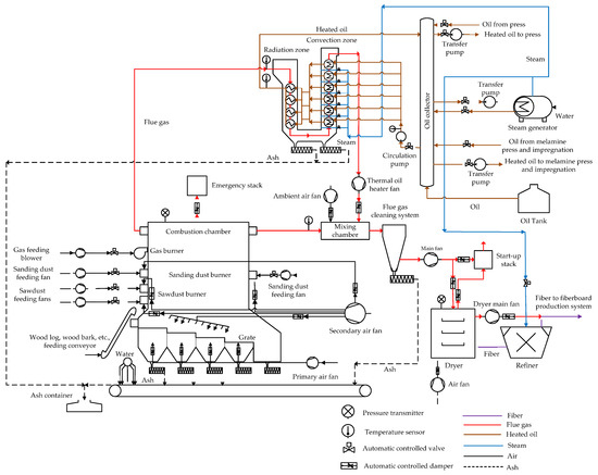
Figure 2.
The process diagram of the thermal energy production system in the factory producing furniture components.
2.2. Data Description
The daily data of the TEPS are provided by the factory producing furniture components in Turkey. The data were collected for the period from 1 June 2018 to 31 December 2019. The averages of hourly observed values were used as the daily data. The dataset was preprocessed to remove errors and outliers. There were 482 convenient data points in the data set. The rates of training and test data were tried in both random and chronological order from 70% to 90% and 10% to 30% in turn until the highest accuracy of each predictive model was attained.
2.3. Variable Selection
The dataset includes 22 inputs: grate load (GL), primary air fan passage ratio (PFPR), sanding dust and sawdust load (SDSL), secondary air fan passage ratio (SFPR), flue gas inlet temperature to radiation (FGTR), flue gas inlet temperature to mixing chamber (FGTMC), ambient air fan passage ratio (AFPR), thermal fan passage ratio (TFPR), internal pressure of boiler (IPB), oil flow rate (OFR), oil inlet temperature to convection (OITC), oil exit temperature from radiation (OETR), boiler stack by-pass damper passage ratio (BSPR), total steam flow to refiner (TSFR), pressure of dryer (PD), dryer stack by-pass damper passage ratio (DSPR), main fan damper passage ratio (MFPR), steam control valve passage ratio (SVPR), heated oil flow rate to press (HOFP), heated oil flow rate to melamine press and impregnation (HOFMI), heated oil flow rate to steam generator (HOFSG), and fiber production rate (FPR). The output is called TEP. The list of the input and output variables and their minimum and maximum values are shown in Table 1 and Table 2. The source of the values of the inputs and output is the SCADA system of TEPS. The SCADA system controls TEP by providing signals at regular intervals. Basic information is collected with the use of sensors placed on the components of TEPS. Daily collected data are categorized for controllable and uncontrollable variables. Controllable variables are symbolized with , while uncontrollable variables are represented with . The values of uncontrollable variables are determined with respect to the demands of the production planning department. TEP is represented with .

Table 1.
List and notations of the inputs.
Table 2.
List and notation of the output.
An industrial grate-fired boiler with a capacity of 75 MW has been established in the factory for the production of thermal energy. Inputs are categorized as controllable variables and uncontrollable variables as presented in Table 1. Some of the system variables are important because they influence each other. For example, the airflow affects biomass combustion, which becomes rapid as the airflow rises. The decision variables PFPR and SFPR are used for the control of airflow to boost TEP. However, AFPR is adjusted with respect to the FGTMC in order to keep the flue gas at a suitable temperature for the fiber drying process. When the wood-based panel production increases, fiber production rises as well. FPR depends on TSFR in the refiner and MFPR of flue gas in the drier. TFPR and MFPR are the decision variables to control the flow of flue gas from convection zone to mixing chamber and from mixing chamber to drier. OITC and OETR are the decision variables to control the increase of oil temperature in TEPS. The quantities of GL and SDSL in the combustion chamber are decided with respect to the need of thermal energy for the production of wood-based panels in the factory. TEP is the output variable representing the sum of heat energy obtained from flue gas, heat energy obtained from heated oil, and steam energy production at the TEPS.
Prediction accuracy can be improved by reducing the number of predictors . Therefore, the importance of predictors can be estimated with RTs by summing changes in the mean square error (MSE) due to splits on every predictor, and dividing the sum by the number of branch nodes. At each node, MSE is estimated as the risk for the node, which is defined as the node error weighted by the node probability. Predictor importance associated with a split is computed as the difference between the MSE for the parent node and the total MSE for the two child nodes. The training dataset is used to evaluate the importance of the predictors [39]. On the other hand, it is also possible to choose the most important variables with RFs. The main idea of predictor importance estimation with RFs is to permute out-of-bag (OOB) data to see how influential the predictor variables in the model are in predicting response [39,40,41].
2.4. Prediction Algorithms
SML algorithms, which include RT, RF, NLR, SVR, and ANN, are used to train and test the predictive models of TEPS. Regression models were chosen as the solution methodology because decision and response variables are continuous.
All of the SML techniques have advantages and disadvantages, which can be more or less important according to the data analyzed and thus have a relative relevance. RTs predict output variables by using the minimization of MSE as the split criterion. The best split is chosen among all variables at each node. RTs are easy to interpret, and their structure is transparent. However, overfitting is possible with deeper RTs. Minor changes in the training data have the potential to create large changes in the prediction results from RT modeling [39]. RF is the collection of independent RTs with a combined prediction result by averaging. RFs reduce the variance in the RTs by using different training samples. The best split is chosen among the subset of randomly selected predictors at each node in the RF algorithm. More RTs in the RF provide a more robust model and prevent overfitting. However, this might slow down the process [42]. NLR is a type of regression analysis in which the response variable is modeled with the successive approximations of non-linear fitting methods. The NLR method can speed up the prediction process, if there are non-linear and non-stationary relationships between the decision variables in the system [43]. SVR provides considerable advantages. The methodology of SVR is based on both mathematical modeling and statistical learning theory, so it can display a very good generalization performance. Its implementation requires relatively simple optimization techniques. However, large data sets require long training times in the SVR approach. It is necessary to choose the best kernel function and hyperparameters for the SVR model in order to improve its prediction accuracy [44]. ANNs offer a number of advantages. Using ANNs makes it possible to detect all of the interactions between predictors. They are capable of relating the inputs to the desired outputs through highly connected networks of neurons to model non-linear systems. They can also be trained with multiple training algorithms. However, the main disadvantages of ANNs are their black-box and experimental nature in modeling with greater computational burden and overfitting [45].
2.4.1. Regression Tree
The response values are predicted with RTs by following the decisions from the root node to leaf node as seen in Figure 3. The stump is the top node and includes all observations of the training data. A predicted response value where is assigned to each terminal node, which is called a leaf.
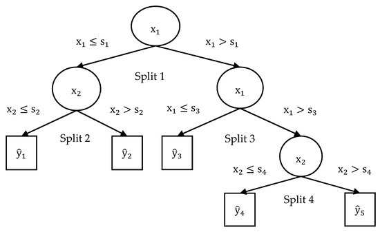
Figure 3.
Geometrical representation of regression trees.
The basıc idea of RTs is that predictor space is segmented into regions . The training data are used to calculate the predicted output as the mean of response variables falling into each region. is the predictor of the RT model given in Equation (1) [39]. characterizes parameters in terms of split variables, cut-off points at each node, and the terminal node values for RTs. is the mean of observed response values in the same region, as seen in Equation (2) [39].
At the tree-growing stage, split nodes are chosen by considering the highest reduction in the MSE between the response values for the training sample and their sample mean at each node. The problem of choosing regions is an NP-hard problem, and its solution is infeasible. For selecting regions in Figure 4, a training error estimate is calculated as the minimization of the MSE as given in Equation (3) [39]. is the number of observations in , while is the number of regions.
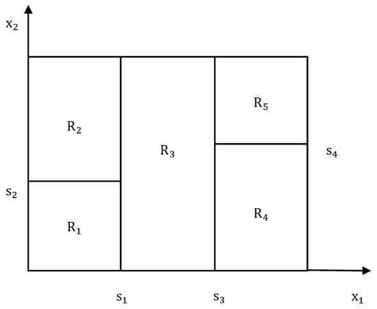
Figure 4.
Graphical representation of recursive binary splitting.
Recursive binary splitting is a greedy algorithm to find the optimal way of partitioning the space of possible values of for the split selection. At each iteration, the optimal cut-off point for is examined in order to choose the predictor that, yields the lowest MSE among inputs. Iterations are terminated when the MSE gain becomes too small [39].
RTs can be pruned by considering the error-complexity measure as given in Equations (4) and (5) [39].
is the error-complexity measure, is the sum of square error of observed responses and predicted responses, is the number of terminal nodes, and is the contribution to the error-complexity measure for each terminal node.
The term in Equation (4) penalizes the over-fitting of RTs. The overfitting emerges by partitioning too finely to grow RTs. AIndependent test data or cross-validated data can be used to choose the right–size of RT. -fold cross-validation can typically be with fold when applied. The proper value of is examined to avoid overfitting. As long as more nodes are added to the RT, the training error becomes unrealistically low. Therefore, the RT with true complexity is the RT minimizing for the proper value of [46]. The flow chart of RTs is presented in Figure 5.
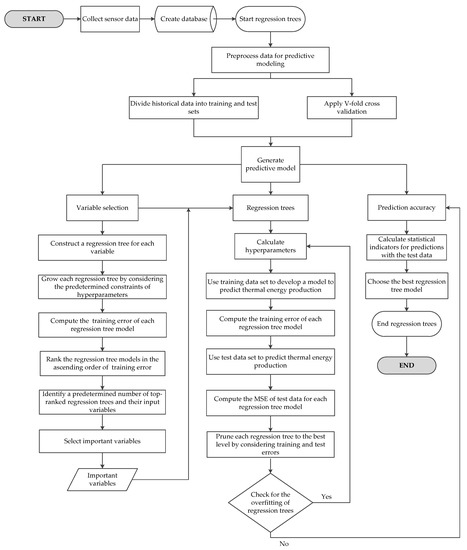
Figure 5.
Flowchart of regression trees.
2.4.2. Random Forest
RF is composed of many RTs. It is a prediction technique derived with the modification of bagging. In bagging, a large collection of decorrelated RTs is built, bagged into one predictor, and averaged to obtain an overall prediction. The prediction in Equation (6) [42,46] is obtained when the RT is applied with the bootstrap sample drawn from the training sample with replacement.
After growing bagged trees , the RF predictor is formulated by averaging predicted values as given in Equation (7) [42,46] to calculate the overall prediction. The variance of the predictor can be calculated as presented in Equation (8) [42,46].
In RFs, it is assumed that are strongly correlated and identically distributed (ID) over bootstrap sample . Each of the predictors has the same variance . The correlation of different predictors is equal to . When the number of trees of the bootstrap samples is increased, becomes lower for different predictors, where . Then, a lower variance on the predictor exists [42,46].
OOB samples, which contain 37% of the whole dataset, are used as the test data of RFs. The error rate for observations that are left out of the bootstrap sample is called the OOB error rate, which is monitored for each RT grown on the bootstrap sample [42]. The flowchart of RFs is shown in Figure 6.
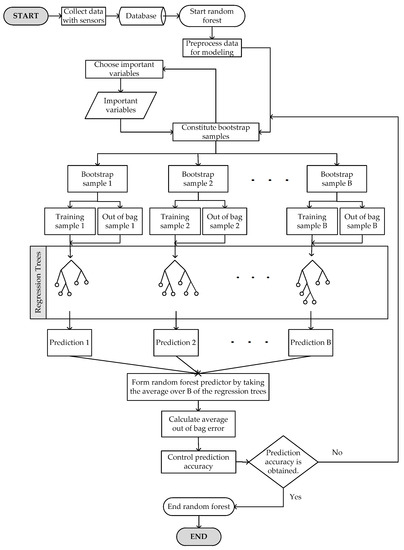
Figure 6.
Flowchart of random forests.
2.4.3. Non-Linear Regression
NLR is a powerful modeling tool, which principally refers to the development of mathematical expressions to describe the behavior of random variables. The unknown parameters in a non-linear model are estimated by minimizing a statistical criterion between observed and predicted values. The relationships between and ’s can be expressed with the function , which can be written as in Equation (9) [43]. includes the parameter vector , which needs to be estimated.
In much of statistical practice, there is a lack of information about the form of the relationship of variables, because the underlying processes are generally complex and not well understood. It is necessary to find some simple function for which Equation (9) holds as closely as possible [43].
The general form of the NLR model is represented with Equations (10) and (11). is the function of independent variables x and parameters . The error term is assumed to be an independently and normally distributed random variable. The non-linear functional form of the NLR model is used to create a prediction model with fewer parameters to obtain a better-characterized response. Equations (10) and (11) are iteratively fit by non-linear least-squares estimation [43]. The flowchart of NLR model is given in Figure 7.
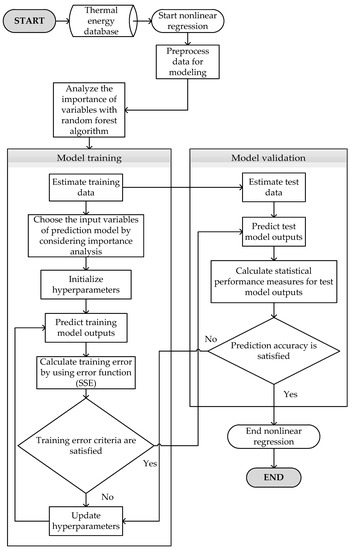
Figure 7.
Flowchart of non-linear regression.
2.4.4. Support Vector Regression
SVR allows for designing prediction models with a large number of variables and small samples owing to its robust pattern. SVR can learn both simple and highly complex regression problems. Sophisticated mathematical principles can be employed with the SVR models to avoid overfitting [46]. It utilizes linear, polynomial, and Gaussian kernels to construct prediction models [44].
denotes the training data where , assuming that is a linear function as presented in Equation (12) [44]. Convex optimization problem (COP) with slack variables searches for the possibility that does not satisfy the constraints for all points as shown in Equation (13) [44].
In Equation (13), the constant is used to determine the trade-off between the flatness of and the tolerable amount of deviations larger than . The COP with slack variables corresponds to the -insensitive loss function. Figure 8 illustrates the -insensitive loss function, which is formulated as given in Equation (14) [46]. is the -insensitive error measure. An function, which deviates from by a value less than for each training point , is found to keep as flat as possible [46].
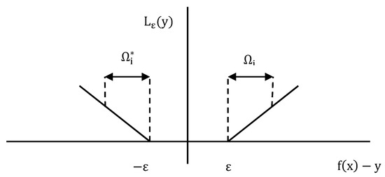
Figure 8.
-insensitive loss function.
COP is computationally simpler to solve in its Lagrangian dual formulation (LDF). If COP satisfies Karush–Kuhn–Tucker (KKT) conditions [46], the solution of the dual problem gives the value of the optimal solution to the primal problem. LDF is obtained from the primal function by introducing non-negative multipliers and for each observation as presented in Equation (15) [44].
Support vectors depending only on kernel functions are given in Equation (16) [44]. They are used to predict response values in the SVR model. The flowchart of the SVR model is shown in Figure 9.
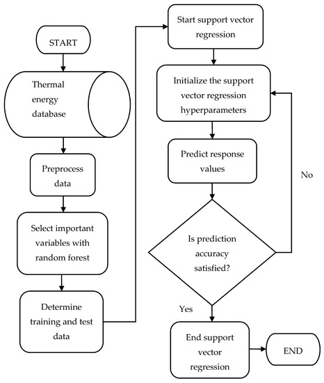
Figure 9.
Flowchart of support vector regression model.
2.4.5. Artificial Neural Networks
ANNs are the mathematical representation of biological nervous systems and can execute complex computational tasks. This article uses MLPNNs, which involve multiple and fully connected input, hidden, and output layers as presented in Figure 10. Each node in the hidden and output layers represents a neuron with linear or sigmoid activation functions [44].
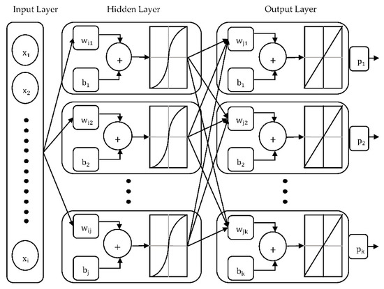
Figure 10.
Schematic diagram of the multilayer perceptron neural network with one hidden layer.
The learning process of MLPNNs is influenced by setting the weight vector on the basis of the comparison of the target and predicted outputs (). denotes the training data with argument value pairs of observed inputs and target outputs . The closeness of the target and predicted outputs can be measured with the non-linear error function (EF) as given in Equation (17), in which are predicted outputs [45].
Firstly, all of the inputs are multiplied by their corresponding weights to form preactivation functions for each neuron. The preactivation values obtained from each neuron are input into the non-linear activation functions . The outputs of each neuron are multiplied by their corresponding weights . Then, weighted values are summed to form the preactivation function of the output neuron. Finally, target output values are computed using the preactivation values in the linear activation function . and are the biases of each neuron in the hidden and output layers, respectively. Related formulations are shown with Equations (18)–(21) [45] with respect to Figure 10.
Back-Propagation Algorithm
The gradient descent algorithms (GDAs) can be used to compute the set of weights minimizing the EF. The EF’s derivatives are taken iteratively with respect to each parameter in the GDAs until the best solution is obtained for error minimization. A back-propagation (BP) algorithm in MLPNNs can be used to determine the influence of weights on the prediction of outputs and to adjust the determined weights regarding the error minimization. The modification of the weights in the first and the second layers can be done with Equations (22) and (23), respectively, with the application of the BP algorithm [45]. represents the learning rate and symbolizes the number of iterations in both equations.
The formulations of the amount of weight corrections in both layers using the gradient of the EF are given in Equations (24) and (25) as follows [45].
The biases of both layers are represented with Equations (26) and (27) as given below [45].
The error signals of both layers are formulated with Equations (28) and (29) [45].
Levenberg–Marquardt Algorithm
The Levenberg–Marquardt (LM) algorithm is an approximation of Newton’s method, which uses a Hessian matrix with the second partial derivatives. The Hessian matrix can be approximated with the formulation in Equation (30) [47].
is the Jacobian matrix that contains the first derivatives of the MLPNN errors with respect to the weights and biases. can be computed through the BP algorithm. On the other hand, the gradient can be computed with the formula in Equation (31), where is the vector of the MLPNN errors [47].
The LM algorithm uses the approximation to the Hessian matrix to update the weights in the MLPNN with Equation (32), where is a constant value [47]. The flowchart of the MLPNN model is presented in Figure 11.
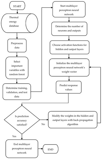
Figure 11.
Flowchart of the multilayer perceptron neural network model.
2.5. Modeling Accuracy
Modeling accuracy of the data-driven models are evaluated with percentage error (PE), fractional bias (FB), root mean square error (RMSE), normalized mean square error (NMSE), and index of agreement (IA). Their formulations are given in Equations (33)–(37) [48]. represents predicted output values. is the observed output value. symbolizes the mean of predicted output values, while is the mean of observed output values. is the number of observations in the test data. IA is an indicator that measures the correlation between the predicted and observed values. IA varies between 0 and 1. When IA takes the value of 1, it results in the best modeling accuracy under the condition of .
2.6. Optimization Model
This article aims to design an optimization model of TEPS in a factory producing furniture components to maximize TEP per unit of wood consumption. A PSO algorithm is proposed to calculate the optimal values of decision variables. The TEPS optimization model is designed as an integrated model of ANN and PSO.
PSO is a stochastic population-based metaheuristic inspired from swarm intelligence. Particles are simple and non-sophisticated agents cooperating by an indirect communication and moving in the decision space. PSO has many similarities with GAs, in which a population of random solutions is initialized to search for optimal solutions by updating generations. However, PSO does not use evolutionary operators such as crossover and mutation. The potential solutions are called particles in the PSO algorithm. A swarm of particles is arbitrarily arranged in the problem space by following the current optimal particles. The particles are progressively in search of different positions and another locally or globally best solution [49].
Shi and Eberhart (1998a, 1998b) [50,51] reported the formulas of the velocity and position of particles with the inclusion of inertia weight in the PSO algorithm as presented in Equations (38) and (39). is selected from the interval of [0.9,1.4]. represents particles, which are potential solutions to problems in the D-dimensional search space. is the velocity along each dimension. Each particle is defined by its position vector . The position of a particle’s best solution is represented by . is the position of the global best solution for all particles. and are cognitive and social parameters, which have positive values, while and denote random numbers uniformly distributed in the interval of [0, 1].
The proposed methodology is an integrated ANN–PSO model to maximize the objective function value. The flow chart of the integrated ANN–PSO model is presented in Figure 12. The PSO model begins by considering the controlling parameters and the initial positions and velocities of particles. After the initiation of the PSO model, an ANN simulation is run with the particle positions obtained by the PSO algorithm to calculate the objective function value for each iteration. Newer objective function values are compared with the existing values obtained in the previous iteration in order to capture the best objective function value. An overall loop is run until the termination criterion is met. The objective function value is identical to fitness value. Finally, global best fitness value is determined.
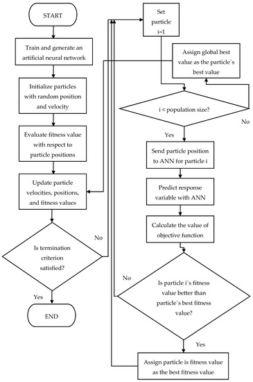
Figure 12.
Flowchart of the integrated artificial neural network and particle swarm optimization algorithm.
3. Results and Discussion
Optimization problems encountered in a large spectrum of industrial applications have a complex pattern. Moreover, it is very difficult to solve them in an exact manner within a reasonable amount of computation time. Approximate algorithms are considered as the main alternative to solve the optimization problems of real-life. TEPS also has processes with non-linear relationships, and physical and chemical reactions. TEP processes must be carefully monitored and controlled to have a stable TEP.
The prediction and optimization of TEPS can be executed with three common approaches, namely analytical, hybrid, and data-driven methods. Analytical methods include mathematical models of processes proceeding in the machines and devices of TEPS. However, in many cases, these processes are complex, and the construction of analytical models of physical processes is not practical because of the expertise required, difficulties in making proper assumptions, very long computation time, and inability to adapt to environmental, economical, and social aspects, especially for the experiments of TEPS operators in the course of production. Hybrid methods of TEPS can be developed with the application of both analytical methods and artificial intelligence methods. Moreover, hybrid methods improve the prediction accuracy and reduce the computational complexity of analytical models. However, hybrid methods still contain the same limitations that usually exist in analytical methods. In contrast, data-driven methods of TEPS involve the ability to tackle the difficulties of analytical methods and hybrid methods. Data-driven methods can provide the possibility to explore statistical patterns even from noisy and incomplete data instead of onsite physical information. From this point of view, an integrated ANN–PSO model for the prediction and optimization of TEPS is designed in this article. After SML energy prediction models are applied for the TEP prediction, the SML model with the best prediction accuracy is determined as the ANN model. Then, daily optimal values of controllable variables and the maximized TEP values per day are calculated with the integrated ANN–PSO model. The ANN–PSO model is a data-driven approach particularly implemented for a real-life case of TEPS in a factory producing furniture components. It is possible to solve optimization problems of TEPS by modifying the implemented ANN-PSO model with respect to the characteristics of the problems to be handled in the design and optimization of TEPS.
Six different models are proposed to predict TEP in this article. The PSO algorithm is used as the single objective optimization model. Prediction models and the integrated ANN-PSO model are implemented in Matlab R2020b version. The experiments were conducted by using a notebook with 2.20 GHz Intel (R) Core (TM) i7-8750H processor and 16.00 GB RAM.
RTs, which grow deeply, are usually accurate for the training data. However, they might not have high accuracy on the test data. It is possible to change the depth of RTs by controlling hyperparameters, namely the maximum number of splits, minimum leaf size, and minimum parent size. For the RTs, minimum leaf size from 1 to 5 and minimum parent size from 5 to 50 are examined. If is the training sample size, the maximum number of splits is limited to . Deep RTs can be pruned to the level with the minimum MSE for training and test data sets to grow shallower RTs. Importance analysis with the RT algorithm is a convenient option to reduce the high dimensionality of inputs in RTs. Training and test data sets of RTs can be chosen either in the chronological or random order. Alternatively, a cross-validation algorithm can be a useful technique to randomly divide the whole data set into folds with approximate sizes to grow RTs. -fold cross-validation grows RTs, and predictions obtained from the cross-validated test data are aggregated with respect to the chronological order in the data set to match them with their observation values. Rates of training data are tried from 70% to 90%. The seed for the random number generator is chosen between 1 and 5.
Table 3 summarizes the RTs with the best prediction performance and their hyperparameters to predict TEP. A pruned regression tree model designed with important predictors (PRTDIP) is proposed to improve the modeling accuracy by using only important predictors GL, MFPR, BSPR, TSFR and HOFSG for the TEP response variable. The importance estimates of each predictor with RTs for TEP are given in Figure 13. The chosen threshold value is 0.5.
Table 3.
Regression tree models to predict thermal energy production.
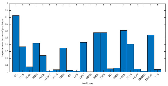
Figure 13.
Importance estimates of predictors with regression trees for thermal energy production.
PRTDIP is grown by using 85% of the data points in the training data set. Training data are selected in random order. There are 77 pruning levels in PRTDIP. The minimum level of the training and test errors emerges at the pruning level of 59. The total computation time is 1.64 s.
A cross-validated shallow regression tree (CVSRT) is built with -fold cross-validation. After RTs are grown, obtained predictions of TEP with the cross-validated test data are aggregated in chronological order. The histogram of the number of splits in the CVSRT shows that the number of imposed splits with the highest frequency is 160 among 10 CVSRT as given in Figure 14. Then, the maximum number of splits is reduced to 79 to search for the reduction of model complexity. The test error of CVSRT model is minimized with the hyperparameters in Table 3. The computation time of the CVSRT model is 1.32 s. The CVSRT model is much less complex and approximates the performance with the PRTDIP model.
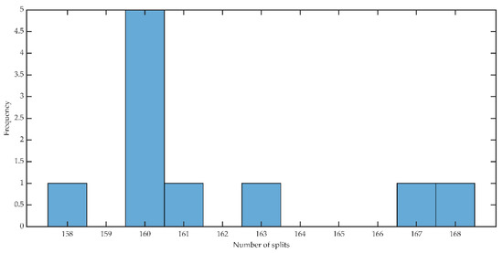
Figure 14.
Histogram of the number of splits on the cross-validated shallow regression tree model for the prediction of thermal energy production.
RFs designed with important predictors (RFDIP) arise from RTs with quantities from 1 to 200 to predict TEP. For each RFDIP, OOB test error is calculated with respect to the minimum leaf size of 5, 10, 20, 50, and 100. Important predictors GL, MFPR, HOFSG, BSPR, OITC, SDSL, and TSFR are chosen with the RF algorithm for TEP. The importance estimates of each predictor are given in Figure 15. The threshold value is taken as 0.5 for importance analyses. The OOB test error is minimized when 200 RTs are grown with the minimum leaf size of 5 as presented in Figure 16. The computation time of the RFDIP model is 38.55 s. OOB predictions are estimated by averaging over predictions from all trees in the ensemble for which these observations are OOB. Then, the OOB predictions are brought together to obtain the holistic data set with 482 data points.
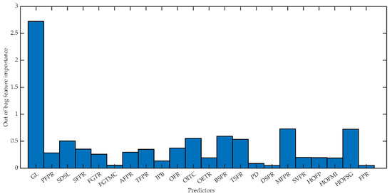
Figure 15.
Importance estimates of predictors with random forests for thermal energy production.
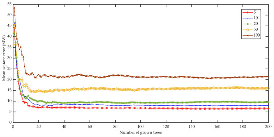
Figure 16.
Choosing the best random forest designed with important predictors model by considering MSE with respect to the number of grown trees and leaf sizes.
The NLR model is designed with fewer parameters to obtain a better-characterized response without overfitting. The NLR models for the prediction of TEP are examined with respect to two predictors. They are randomly chosen among the most important predictors determined with the RF algorithm in Figure 15. The cross-validation approach is also tried with the whole data set. The most accurate NLR model to predict TEP is obtained as , which is designed with the predictors GL and MFPR. The rates of training and test data are 80% and 20%, respectively in the chronological order for the best NLR model, for which parameters , , , and are significantly estimated with p-values far less than 0.05. The total time of computation is 1.20 s.
The SVR models are designed with 22 predictors. Linear, polynomial, and Gaussian kernels are tried with the SVR models. Kernel functions are tested to specify the best parameter settings for the box constraint from 0.001 to 1000, kernel scale from 0.001 to 1000, epsilon from 0.0078 to 780, and polynomial order from 2 to 4. The SVR model designed with 22 predictors, a training data rate of 90%, and a test data rate of 10% provides the best prediction results for TEP. The best SVR model uses the polynomial kernel function with the parameters of polynomial order, box constraint, kernel scale, and epsilon as 3, 1, 1, and 0.7805, respectively. The total time of computation is 1.43 s.
The MLPNN with the BP algorithm is modeled with 22 predictors. Training, validation, and test data are constituted with both random and specified indices. The LM algorithm is used as the training algorithm. Batch training with all of the inputs is used to update weights and biases in the ANN model. MSE is the error function. Different numbers of hidden layers are tried from 1 to 15, and different numbers of neurons in hidden layers are tried from 5 to 50. Each neuron in hidden layers includes either hyperbolic tangent sigmoid or log-sigmoid transfer functions, while in output layers it uses a linear transfer function.
The MLPNN models were tried 50 times to find the ANN with the best prediction performance. The MLPNN model with the best prediction performance for TEP contains 22 inputs, 1 hidden layer, and 5 neurons in the hidden layer. Training, validation, and test datasets of the best MLPNN model are created with the rates of 70%, 10%, and 20%, respectively, with specified indices.
Table 4 summarizes the modeling performance of all prediction models tested for TEP. The MLPNN model, for which IA takes the value of 1.00 under the condition of , offers a better prediction accuracy than the other models. The MLPNN model is more prominent, with significantly lower RMSE and PE indicators than the values attributed to the other algorithms. The total computation time of the MLPNN model for TEP is 1.64 s. The ANN model providing the highest prediction accuracy without overfitting is saved to integrate with the PSO model.
Table 4.
Modeling accuracy of the prediction models.
Figure 17 shows the test observations against their predicted values by the MLPNN prediction model for TEP. The statistical indicators and MLPNN structure show that the MLPNN model perfectly predicts the TEP with time, as seen in Figure 17. All of the TEP patterns and peaks for 96 points in the test data are clearly recognized by the proposed prediction model.
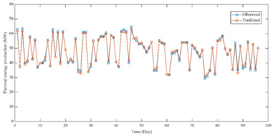
Figure 17.
Observed and predicted values of thermal energy production for multilayer perceptron neural network model.
The control of a TEPS requires analytical models for heat transfer and combustion processes that initialize in grate-fired boilers. However, the construction of analytical models is difficult and time-consuming in the on-site experiments of operators because of the complexity of these processes. Thus, this article proposes an optimization model for TEPS using ANN and PSO to improve the capability of operators for system optimality. Regarding the good agreement between the observed and predicted values as presented in Figure 17, it is seen that the complexity of TEPS is clearly described with the MLPNN approach. The SCADA system and reliable sensors are extensively useful for monitoring a TEPS. The operators of a TEPS can control processes by adapting the system variables to any uncertainties of the characteristics of influent biomass, biomass feeding cycles, combustion stability, air disturbance, furnace wall conditions, etc. from the SCADA system in order to reach the maximum TEP with operator experience and process knowledge. However, an integrated ANN–PSO model is proposed to research the optimality conditions of TEPS for the maximization of TEP in this article. The proposed optimization model can be utilized to improve the control ability of operators for the maximization of TEP in practice.
The proposed optimization model aims to find the daily optimal values of controllable variables to maximize TEP per hour for each day. The single objective function with constraints is formulated in Equation (40) as a maximization problem.
TEP is a function of both controllable and uncontrollable variables. The description of both types of variables is provided in Table 1. PFPR, SFPR, FGTR, FGTMC, AFPR, TFPR, IPB, OFR, OITC, OETR, BSPR, DSPR, MFPR, and SVPR are selected as controllable variables for the model. The uncontrollable variables are GL, SDSL, TSFR, PD, HOFP, HOFMI, HOFSG, and FPR.
Each controllable variable is optimized subject to the constraint between its minimum and maximum observed values in the dataset. The minimum and maximum observed values of the inputs and the output of the TEPS are also presented in Table 1. Swarm size, maximum velocity, inertia weight, and maximum iteration number are sequentially set to 10, 0.09, 1.2, and 10, respectively, for the PSO algorithm. The steps shown in the flow chart of the integrated ANN–PSO model in Figure 12 are repeated until the termination criterion is met. Operational conditions of TEPS in a factory producing furniture components remain unchanged as much as possible for a full season to obtain a stable TEP.
The daily optimization results of the TEP obtained with the proposed ANN–PSO model are presented in Figure 18. The test data including 96 observations with specified indices are used to solve the maximization problem represented with Equation (40) by using the integrated ANN–PSO model. With each iteration, the trained ANN is used to predict the TEP based on controllable and uncontrollable decision variables. Then, the PSO algorithm determines the best fitness value for the TEP by finding the optimal settings of controllable variables. Uncontrollable variables are also used in the ANN–PSO model with their observed values, but they are not optimized. The elapsed time to solve the TEP maximization problem with the integrated ANN–PSO model is 913 s.
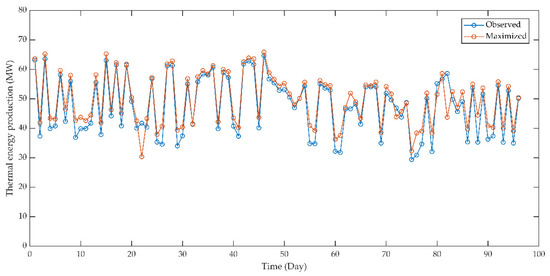
Figure 18.
Observed and maximized values of thermal energy production.
Under the optimized operational conditions determined with the integrated ANN–PSO model, TEP can be improved by 4.24%. The increased TEP is owing to the optimization of controllable variables based on the maximization model in Equation (40). Figure 18 illustrates that most of the maximized TEP per hour for each day is larger than the daily observed values. Moreover, the production for the test period shows similar variability to the actual values on a daily basis. The stability of TEP is beneficial for the TEP process and factory operations. The integrated prediction and optimization model of TEPS in a factory producing furniture components is built and implemented by using ANN and PSO algorithms, and the maximized TEP is obtained in case of the optimization of all controllable variables at the same time for daily TEPS operations in this article.
4. Conclusions
The results obtained by this article prove that TEPS, which involves complex operations with chemical and physical reactions, can be modeled and optimized with very high prediction accuracy, low complexity, and short computation time by using the integrated ANN-PSO model. The solution of the single-objective optimization model has resulted in a 4.24% increase in the TEP under optimized operational conditions.
By putting the integrated ANN–PSO model into practice, it is expected that the TEPS will contribute to the cleaner production in the factory producing furniture components with maximized TEP, improved recycling of wood waste, and efficient usage of cleaner technologies at optimal input settings. It is recommended that education and orientation sessions about the application of the proposed optimization model are organized for the TEPS operators.
The integrated ANN-PSO model, which is implemented in this article, is intrinsic to the TEPS. Therefore, it is necessary to redesign the proposed optimization model with respect to the features of another energy production system in the case of its application for optimization problems in other high-energy consumer industries.
The proposed single objective ANN–PSO model can be customized to design a multi-objective metaheuristic optimization model of TEPS as a future study.
Author Contributions
Conceptualization, H.A.; methodology, H.A. and G.Ö.; software, H.A.; validation, H.A.; formal analysis, H.A.; investigation, H.A.; resources, H.A.; data curation, H.A.; writing—original draft preparation, H.A.; writing—review and editing, H.A.; visualization, H.A.; supervision, G.Ö.; project administration, G.Ö.; funding acquisition, G.Ö. All authors have read and agreed to the published version of the manuscript.
Funding
This research was supported by the Research Fund of Süleyman Demirel University, project number FDK-2018-6845.
Acknowledgments
The authors would like to express appreciation to Süleyman Demirel University for their administrative, technical and equipment supports under project number FDK-2018-6845.
Conflicts of Interest
The authors declare no conflict of interest.
References
- Yin, C.; Rosendahl, L.A.; Kaer, S.K. Grate-firing of biomass for heat and power production. Prog. Energy Combust. Sci. 2008, 34, 725–754. [Google Scholar] [CrossRef]
- Kim, M.H.; Song, H.B. Analysis of the global warming potential for wood waste recycling system. J. Clean. Prod. 2014, 69, 199–207. [Google Scholar] [CrossRef]
- Sulaiman, C.; Abdul-Rahim, A.S.; Ofozor, C.A. Does wood biomass energy use reduce CO2 emissions in European Union member countries? Evidence from 27 members. J. Clean. Prod. 2020, 253, 119996. [Google Scholar] [CrossRef]
- Bridgwater, A.V. Renewable fuels and chemicals by thermal processing of biomass. Chem. Eng. J. 2003, 91, 87–102. [Google Scholar] [CrossRef]
- Osman, A.I.; Abdelkader, A.; Farrell, C.; Rooney, D.; Morgan, K. Reusing, recycling and up-cycling of biomass: A review of practical and kinetic modelling approaches. Fuel Process. Technol. 2019, 192, 179–202. [Google Scholar] [CrossRef]
- Costa, M.; Massarotti, N.; Indrizzi, V.; Rajh, B.; Yin, C.; Samec, N. Engineering bed models for solid fuel conversion process in grate-fired boilers. Energy 2014, 77, 244–253. [Google Scholar] [CrossRef]
- Cai, Y.; Tay, K.; Zheng, Z.; Yang, W.; Wang, H.; Zeng, G. Modeling of ash formation and deposition processes in coal and biomass fired boilers: A comprehensive review. Appl. Energy 2018, 230, 1447–1544. [Google Scholar] [CrossRef]
- Rezeau, A.; Diez, L.I.; Royo, J.; Diaz-Ramirez, M. Efficient diagnosis of grate-fired biomass boilers by a simplified CFD-based approach. Fuel Process. Technol. 2018, 171, 318–329. [Google Scholar] [CrossRef]
- Yin, C.; Rosendahl, L.; Kaer, S.K.; Clausen, S.; Hvid, S.L.; Hille, T. Mathematical modeling and experimental study of biomass combustion in a thermal 108 MW grate-fired boiler. Energy Fuels 2008, 22, 1380–1390. [Google Scholar] [CrossRef]
- Haberle, I.; Skreiberg, O.; Lazar, J.; Haugen, N.E.L. Numerical models for thermochemical degradation of thermally thick woody biomass, and their application in domestic wood heating appliances and grate furnaces. Prog. Energy Combust. Sci. 2017, 63, 204–252. [Google Scholar] [CrossRef]
- Bermudez, C.A.; Porteiro, J.; Varela, L.G.; Chapela, S.; Patino, D. Three-dimensional CFD simulation of a large-scale grate-fired biomass furnace. Fuel Process. Technol. 2020, 198, 106219. [Google Scholar] [CrossRef]
- Yin, C.; Kaer, S.K.; Rosendahl, L.; Hvid, S.L. Co-firing straw with coal in a swirl-stabilized dual-feed burner: Modelling and experimental validation. Bioresour. Technol. 2010, 101, 4169–4178. [Google Scholar] [CrossRef] [PubMed]
- Ranzi, E.; Pierucci, S.; Aliprandi, P.C.; Stringa, S. Comprehensive and detailed kinetic model of a traveling grate combustor of biomass. Energy Fuels 2011, 25, 4195–4205. [Google Scholar] [CrossRef]
- Kusiak, A.; Smith, M. Data mining in design of products and production systems. Annu. Rev. Control. 2007, 31, 147–156. [Google Scholar] [CrossRef]
- Mishra, S.; Tripathy, H.K.; Mallick, P.K.; Bhoi, A.K.; Barsocchi, P. EAGA-MLP- An enhanced and adaptive hybrid classification model for diabetes diagnosis. Sensors 2020, 20, 4036. [Google Scholar] [CrossRef] [PubMed]
- Sun, T.; Xia, B.; Liu, Y.; Lai, Y.; Zheng, W.; Wang, H.; Wang, W.; Wang, M. A novel hybrid prognostic approach for remaining useful life estimation of lithium-ion batteries. Energies 2019, 12, 3678. [Google Scholar] [CrossRef]
- Rushdi, M.A.; Rushdi, A.A.; Dief, T.N.; Halawa, A.M.; Yoshida, S.; Schmehl, R. Power prediction of airborne wind energy systems using multivariate machine learning. Energies 2020, 13, 2367. [Google Scholar] [CrossRef]
- Yoo, K.; Shukla, S.K.; Ahn, J.J.; Oh, K.; Park, J. Decision tree-based data mining and rule induction for identifying hydrogeological parameters that influence groundwater pollution sensitivity. J. Clean. Prod. 2016, 122, 277–286. [Google Scholar] [CrossRef]
- Mihaita, A.S.; Dupont, L.; Chery, O.; Camargo, M.; Cai, C. Evaluating air quality by combining stationary, smart mobile pollution monitoring and data-driven modelling. J. Clean. Prod. 2019, 221, 398–418. [Google Scholar] [CrossRef]
- Chen, Y.K.; Chiu, F.R.; Chang, Y.C. Implementing green supply chain management for online pharmacies through a VADD inventory model. Int. J. Environ. Res. Public Health 2019, 16, 4454. [Google Scholar] [CrossRef]
- Kalogirou, S.A. Artificial intelligence for the modeling and control of combustion processes: A review. Prog. Energy Combust. Sci. 2003, 29, 515–566. [Google Scholar] [CrossRef]
- Chu, J.Z.; Shieh, S.S.; Jang, S.S.; Chien, C.I.; Wan, H.P.; Ko, H.H. Constrained optimization of combustion in a simulated coal-fired boiler using artificial neural network model and information analysis. Fuel 2003, 82, 693–703. [Google Scholar] [CrossRef]
- Hao, Z.; Qian, X.; Cen, K.; Jianren, F. Optimizing pulverized coal combustion performance based on ANN and GA. Fuel Process. Technol. 2003, 85, 113–124. [Google Scholar] [CrossRef]
- Rusinowski, H.; Stanek, W. Neural modelling of steam boilers. Energy Convers. Manag. 2007, 48, 2802–2809. [Google Scholar] [CrossRef]
- Chandok, J.S.; Kar, I.N.; Tuli, S. Estimation of furnace exit gas temperature (FEGT) using optimized radial basis and back-propagation neural networks. Energy Convers. Manag. 2008, 49, 1989–1998. [Google Scholar] [CrossRef]
- Gu, Y.; Zhao, W.; Wu, Z. Online adaptive least squares support vector machine and its application in utility boiler combustion optimization systems. J. Process. Control. 2011, 21, 1040–1048. [Google Scholar] [CrossRef]
- Liukkonen, M.; Heikkinen, M.; Hiltunen, T.; Halikka, E.; Kuivalainen, R.; Hiltunen, Y. Artificial neural networks for analysis of process states in fluidized bed combustion. Energy 2011, 36, 339–347. [Google Scholar] [CrossRef]
- Lv, Y.; Liu, J.; Yang, T.; Zeng, D. A novel least squares support vector machine ensemble model for NOx emission prediction of a coal-fired boiler. Energy 2013, 55, 319–329. [Google Scholar] [CrossRef]
- Gatternig, B.; Karl, J. Prediction of ash-induced agglomeration in biomass-fired fluidized beds by an advanced regression-based approach. Fuel 2015, 161, 157–167. [Google Scholar] [CrossRef]
- Toth, P.; Garami, A.; Csordas, B. Image-based deep neural network prediction of the heat output of a step-grate biomass boiler. Appl. Energy 2017, 200, 155–169. [Google Scholar] [CrossRef]
- Böhler, L.; Görtler, G.; Krail, J.; Kozek, M. Carbon monoxide emission models for small-scale biomass combustion of wooden pellets. Appl. Energy 2019, 254, 113668. [Google Scholar] [CrossRef]
- Yang, T.; Ma, K.; Lv, Y.; Bai, Y. Real-time dynamic prediction model of NOx emission of coal-fired boilers under variable load conditions. Fuel 2020, 274, 117811. [Google Scholar] [CrossRef]
- Hao, Z.; Kefa, C.; Jianbo, M. Combining neural network and genetic algorithms to optimize low NOx pulverized coal combustion. Fuel 2001, 80, 2143–2169. [Google Scholar] [CrossRef]
- Si, F.; Romero, C.E.; Yao, Z.; Schuster, E.; Xu, Z.; Morey, R.L.; Liebowitz, B.N. Optimization of coal-fired boiler SCRs based on modified support vector machine models and genetic algorithms. Fuel 2009, 88, 806–816. [Google Scholar] [CrossRef]
- Zhou, H.; Zhao, J.P.; Zheng, L.G.; Wang, C.L.; Cen, K.F. Modeling NOx emissions from coal-fired utility boilers using support vector regression with ant colony optimization. Eng. Appl. Artif. Intell. 2012, 25, 147–158. [Google Scholar] [CrossRef]
- Wang, C.; Liu, Y.; Zheng, S.; Jiang, A. Optimizing combustion of coal fired boilers for reducing NOx emission using gaussian process. Energy 2018, 153, 149–158. [Google Scholar] [CrossRef]
- Shi, Y.; Zhong, W.; Chen, X.; Yu, A.B.; Li, J. Combustion optimization of ultra supercritical boiler based on artificial intelligence. Energy 2019, 170, 804–817. [Google Scholar] [CrossRef]
- Piekarski, C.M.; de Francisco, A.C.; da Luz, L.M.; Kovaleski, J.L.; Silva, D.A.L. Life cycle assessment of medium-density fiberboard (MDF) manufacturing process in Brazil. Sci. Total Environ. 2017, 575, 103–111. [Google Scholar] [CrossRef]
- Breiman, L.; Friedman, J.H.; Olshen, R.A.; Stone, C.J. Classification and Regression Trees, 1st ed.; Pacific Grove: Wadsworth, OH, USA, 1984. [Google Scholar]
- Loh, W.Y.; Shih, Y.S. Split selection methods for classification trees. Stat. Sin. 1997, 7, 815–840. [Google Scholar]
- Loh, W.Y. Regression trees with unbiased variable selection and interaction detection. Stat. Sin. 2002, 12, 361–386. [Google Scholar]
- Breiman, L. Random forests. Mach. Learn. 2001, 45, 5–32. [Google Scholar] [CrossRef]
- Seber, G.A.F.; Wild, C.J. Nonlinear Regression, 1st ed.; John Wiley & Sons: Hoboken, NJ, USA, 2003. [Google Scholar]
- Vapnik, V. The Nature of Statistical Learning Theory, 1st ed.; Springer: New York, NY, USA, 1995. [Google Scholar]
- Haykin, S. Neural Networks and Learning Machines, 3rd ed.; Pearson Prentice Hall: Hoboken, NJ, USA, 2009. [Google Scholar]
- Hastie, T.; Tibshirani, R.; Friedman, J. The Elements of Statistical Learning: Data Mining, Inference and Prediction, 1st ed.; Springer: New York, NY, USA, 2001. [Google Scholar]
- Hagan, M.T.; Menhaj, M.B. Training feedforward networks with the marquardt algorithm. IEEE Trans. Neural Netw. 1994, 5, 989–993. [Google Scholar] [CrossRef] [PubMed]
- Kusiak, A.; Wei, X. Prediction of methane production in wastewater treatment facility: A data-mining approach. Ann. Oper. Res. 2014, 216, 71–81. [Google Scholar] [CrossRef]
- Kennedy, J.; Eberhart, R.C. Particle Swarm Optimization. In Proceedings of the IEEE International Conference on Neural Networks, Perth, Australia, 27 November–1 December 1995; pp. 1942–1948. [Google Scholar]
- Shi, Y.; Eberhart, R. A Modified Particle Swarm Optimizer. In Proceedings of the IEEE International Conference on Evolutionary Computation, Anchorage, AK, USA, 4–9 May 1998; pp. 69–73. [Google Scholar]
- Shi, Y.; Eberhart, R. Parameter Selection in Particle Swarm Optimization. In Proceedings of the 7th International Conference on Evolutionary Programming, San Diego, CA, USA, 25–27 March 1998; pp. 591–600. [Google Scholar]
Publisher’s Note: MDPI stays neutral with regard to jurisdictional claims in published maps and institutional affiliations. |
© 2020 by the authors. Licensee MDPI, Basel, Switzerland. This article is an open access article distributed under the terms and conditions of the Creative Commons Attribution (CC BY) license (http://creativecommons.org/licenses/by/4.0/).