Article

Study and Simulation of a Wind Hydro Isolated Microgrid

Departamento de Ingeniería Eléctrica, Electrónica y de Control, ETSII UNED, 28040 Madrid, Spain
*
Author to whom correspondence should be addressed.
Energies 2020, 13(22), 5937; https://doi.org/10.3390/en13225937
Submission received: 6 October 2020 / Revised: 9 November 2020 / Accepted: 11 November 2020 / Published: 13 November 2020
(This article belongs to the Special Issue Modeling, Simulation and Control of Wind Diesel Power Systems)

Abstract

:
Isolated microgrids are microgrids which operate autonomously. This paper presents an isolated microgrid which combines a Hydraulic Turbine Generator (HTG) with a Wind Turbine Generator (WTG) to supply consumers forming a Wind Hydro Isolated Microgrid (WHIM). The WHIM includes a Dump Load (DL) to dissipate the active power excess. The WHIM has been modeled and its operation has been simulated in two modes: Wind-Hydro (WH), where both HTG and WTG supply power, and Wind-Only (WO) mode, where the WTG is the active power supplier and the HTG keeps connected to the grid with null power to generate the grid voltage. In WO, a fast frequency regulation is achieved by means of a controller which commands the DL to consume the WTG power excess. Additionally, the simulation of the mode transition from WO to WH, which is triggered by a system active power deficit in WO mode, is shown. A kick starting system designed to speed up the HTG power production improves the transient from WO to WH mode change. Finally, the simulations in WH mode show the interaction between the HTG and WTG. The two controls proposed have been proved effective and the simulations show a good WHIM dynamic performance.

1. Introduction

Isolated microgrids are microgrids which operate autonomously and are located in remote places [1,2,3]. Remote isolated microgrids have been mostly based on Diesel Generators (DG), which can be combined with sources of renewable energy, such as photovoltaic or wind [4] and short-term energy storage systems (ESS), mainly based on flywheels [5] or batteries [6,7]. When an isolated microgrid includes renewables and does not include a DG, it has to include another source of controlled generation, such as a fuel cell [8]. Among the renewable energies, hydro power is the only one that can produce fully controlled power. Hydro power is site-dependent since a river and the possibility of building a dam are needed. Wind power is also site-dependent, since the wind resource is needed at the considered place and, depending on the type of WTG used, can go from uncontrolled to partly controlled generation.
Figure 1 shows the isolated microgrid modeled and simulated in this paper, which combines hydro and wind power. It consists of a Hydraulic Turbine Generator (HTG), a Wind Turbine Generator (WTG), consumer load and a Dump Load (DL). The HTG comprises a Hydraulic Turbine (HT) which drives a Synchronous Machine (SM). The constant speed type WTG of Figure 1 comprises a fixed pitch Wind Turbine (WT) which drives an Induction Generator (IG). Both the HTG and the WTG are combined to form a Wind Hydro Isolated Microgrid (WHIM) to supply the isolated consumers. The DL comprises a resistor bank and a set of power switches and consumes active power when an excess of system active power exists.
In the WHIM of Figure 1, the HTG is always running and connected to the isolated grid, since the SM creates the grid voltage waveform and the SM voltage regulator performs the system voltage regulation. Three operation modes are possible for the WHIM, shown in the figure: Hydro Only (HO), Wind Hydro (WH) and Wind Only (WO). In the HO mode, the HTG supplies all the consumer’s demanded active and reactive power and the WTG is disconnected ( I T = OFF in Figure 1). In this mode, the WHIM behaves as an isolated hydropower system. Frequency regulation is performed by means of the HT speed governor, which actuates on the flow rate entering the HT, by means of a valve, to control the HT mechanical power produced. When the wind speed is above the WT cut-in speed, the WTG is able to supply power, so it is connected to the isolated grid changing to the WH mode. In the WH mode, the WTG supplies active power according to the existing wind speed and the HTG controls its active power to cover the active power net demand. Frequency regulation is achieved as in HO mode. In WH mode, the WTG produced power, P T , can exceed that consumed by the load, P L , ( P T > P L ) and if this happens, the DL must consume the WTG active power excess P T P L to guarantee the power system stability. If the condition P T > P L persists, the WHIM is changed to WO mode. In WO mode, the WTG supplies the active power and the HTG keeps running with null flow rate and therefore null active power, in order to generate the grid voltage and supply reactive power. Frequency regulation is performed in this case by making the DL consume the WTG active power excess. If the WTG generated power falls below the power consumed by the load, then the HTG, that is already connected to the microgrid, must supply active power and the WHPS must change to WH mode.
HO mode is equivalent to an isolated Hydro Power System (HPS) and many small HPS operate isolated [9]. In some small isolated HPS [10] the HT has no flow regulation, so there is no active power regulation and the HTG works permanently at full power. In these cases, frequency regulation is performed by controlling the power consumed by the DL, so that the instantaneous sum of the power absorbed by the consumer load and the power dissipated in the DL is equal to the power generated by the HTG. A simulation example of this DL use in an isolated HPS can be found in [11]. This DL use is analogous to the use of the DL in the WO mode presented in this article, but with the difference that the WTG type used in this article produces non-controllable active power. In WH mode, the HTG counteracts the load and WTG power variations. In a previous paper published by one of the authors [12], a WHIM is modeled, but no DL is considered in the simulations. In that reference, WHIM transients in response to load increase in HO and WH modes are compared, and a better behavior in WH mode, due to the WTG damping action, is found. The WHIM model and its associated controls in this article are focused to allow operation in WO mode and to transition from WO to WH modes. WO mode simulations have been considered in several papers, both with systems which have a backup generator, such as a DG [13,14], or with systems where the WTG is the only power source [15,16]. When an isolated wind power system has no backup generator, it is mandatory for good system performance to include some energy storage: reference [15] includes a flywheel ESS whereas [16] includes a battery plus a supercapacitor ESS.
WHIM can be combined with other conventional power sources, as it is done at the wind-hydro-diesel isolated power system of el Hierro Island in Spain, which also includes a hydropower pumped-storage. The diesel off mode of El Hierro power system has been simulated in several papers, which mainly study the wind-hydro-pumped storage combination. Reference [17] studies the WO mode and shows the use of fixed and variable speed pumps integrated within the hydropower pumped-storage to regulate the system frequency. Reference [18] also studies the WO mode and a flywheel ESS is included in the simulations and different alternative frequency control schemes are studied and compared. References [17,18] show, among others, graphs of system frequency and active powers of the WTGs and pumps, but none of system voltage waveforms. The WHIM considered in this article has neither pump storage nor short-term energy storage and uses the DL as the variable controlled load to absorb the WTG power excess, being the lowest cost solution of all. Additionally, graphs of system voltage will be shown in the simulations section as high order electrical models for the electrical machines are used. In [19], logistic simulations of the El Hierro wind-hydro-diesel power plant in several operational modes are carried out in order to calculate the efficiency and the percentage of load demand covered by renewables in the different operational modes considered.
This article’s main contribution is to present comprehensive simulations of a WHIM. These simulations firstly cover WO mode operation. In it, frequency regulation is achieved by means of the DL while the HTG actuates providing the grid voltage and as a backup generator. Secondly, the transition from WO mode to WH mode, which is triggered by the lack of system active power in WO mode, is simulated. Finally, WH mode is also simulated, and the interaction between the HTG and WTG is shown. Additionally, this article contributes with a proposal of a fast DL frequency regulator, which is active in WO mode, a control logic to start the WO to WH transition, and a control system aimed to speed up and smooth the transition from WO mode to WH mode.
Following this introductory section, this article is organized as follows: Section 2 presents the model of the HTG, along with a discussion on the most appropriate HT type for the WH and WO modes of operation and the models for the WTG and DL; Section 3 presents Simulink schematics for the simulated WHIM, along with the controls needed to operate in WO mode and to smooth the WO mode to WH mode transition; Section 4 presents the different simulation cases considered and mentioned above and, finally, Section 5 concludes with the main contributions of the paper.

2. WHIM Modeling

2.1. The HTG Model

A hydraulic turbine (HT) converts energy from falling water into rotating shaft power [10]. The HT model used in this article is nonlinear, since the simulations consider large variations for the HT operating point. The equations below, in per unit (p.u) values, describe the HT nonlinear model. Their derivation can be obtained from the references [12,20]:
q = y h
P h m e c = A t η q h K D y ( ω 1 )
Equation (1) describes the valve which regulates the flow rate q to the HT. In it, y is the turbine gate opening position that can vary from 0 (fully closed) to 1 (fully open); q = Q / Q b a s e , is the flow rate p.u., Q being the flow rate passing through the turbine and Q b a s e the turbine flow rate with the gate fully open, h = H / H b a s e is the pressure head of water p.u., with H as the pressure head in the turbine admission and H b a s e the total available static head above the turbine [20]. Equation (2) gives the mechanical power p.u. produced by the HT, P h m e c , which has two terms. The first term is the power produced by the flow rate p.u q, with an effective pressure head of water in p.u. h and η is the turbine hydraulic efficiency. A t is a proportionality factor which depends on the HT active rated power and the SM apparent rated power. The second term accounts for a speed deviation effect ( ω 1 ) where ω is the HT shaft speed p.u; 1 p.u. is the rated turbine speed and K D , the damping torque coefficient [20].
The penstock is the pressure pipe that delivers water from the dam to the turbine admission. The following equation, describing the penstock model, was previously derived in [12,20]:
d q d t = 1 T w 1 h h f
In it, h f is the head loss due to friction in the penstock and T w is the water time constant or water starting time in seconds, defined as:
T w = L A g Q b a s e H b a s e
where L, in m and A, in m2, are the penstock length and area, respectively, and g is the gravitational acceleration. Equation (3) is valid for penstocks of short length, in which the pressure wave effects can be neglected.
In WH mode, the HTG must supply the grid with an amount of power equal to the difference between the consumer load and the WTG supplied power. The HT working power range can therefore be very broad and the low load regime can be very common. The efficiency of a HT depends mainly on the flow rate [10]. The HT efficiency is null for flow rates ranging from zero to the no-load flow rate q n l . Different types of hydro-turbines, such as Pelton, Crossflow, Francis, Kaplan, etc. have different q n l and efficiency curves. Due to the highly variable working regime of the HT in WH mode, a good efficiency for q > q n l is the main requirement for the HT in the study considered here. Additionally, in WO mode, as commented before, the HT runs with zero flow rate. When the WHIM is in WO mode and the WTG active power falls below the consumer load, the system frequency will fall and the WHIM must transition from WO to WH mode, ordering the HTG to supply power. In order to supply power, the HT speed governor must increase the flow rate from zero. The time spent to take the flow rate from zero to q n l is a dead time in which the HT is not producing any power and the system frequency will continue falling. The bigger q n l , the longer the dead time, and the worse will be the system transient. Therefore, an HT with a small q n l is needed to improve the WO to WH modes transition. Among the different HT types, the ones that most comply with the previous requirements are Crossflow and Pelton impulse type turbines, Pelton type HT having better efficiency figures than Crossflow type HT. A Pelton type HT has, therefore, been considered in this article. Figure 2 depicts the Pelton turbine efficiency curve used in this article, as a function of q, in abscissa, where q n l is 0.1 p.u.
The HT mechanical output power is converted into electrical power by the SM. The SM must be permanently connected to the isolated grid as it generates the isolated grid voltage waveform. To allow the SM automatic voltage regulator control the system voltage within allowable limits, the SM speed has to always be close to its rated speed. The SM nominal power P S M N O M is 300 kVA, which is enough to provide the microgrid with all the active and reactive power demanded. Since the system frequency is f = 50 Hz and the SM has p = 16 pole pairs, calculating the synchronous speed, n, as n = 60 f / p , the HTG rated speed, n r e f , results in 187.5 rpm. Inertia constant H for low speed HTGs (<200 rpm), ranges between 2–3 s [21], so 2 s is assigned to H H T G , as this article’s HTG is a low power one.

2.2. The WTG Model

The WTG in Figure 1 is a fixed-pitch WT driving an Induction Generator (IG) directly connected to the autonomous grid. Both elements, WT and IG, form a constant-speed stall-controlled WTG. The mechanical power extracted from the wind by the wind turbine, as stated by [22], is
P t m e c = C p P w i n d = C p 1 2 ρ A v 3
where the power coefficient, C p , represents the ratio of the power extracted from the wind to the power available in the wind. The power available in the wind, P w i n d , can be calculated as half of the air density ρ , times the blade swept area A, times the cube of the wind speed v. In the absence of pitch regulation and due to the very limited IG speed range variation, C p can be considered, as a first approximation, a function of the wind speed only. As the wind speed is quasi-random, the active power generated by the WTG will be uncontrolled. The stall-controlled WT model simulated here follows the description presented in [23]. The IG has a rated power of 275 kW (WTG rated power P T N O M = 275 kW), which is enough to supply all the active power demanded in WO mode, and since it consumes reactive power, a capacitor bank is included in Figure 1 to improve the power factor. Inertia constant H w values for WTGs range from 2 to 6 s [24], so 2 s is assigned to H w , as this article’s WTG is a low power one.

2.3. The DL Model

The Dump Load (DL) is used in the WHIM to artificially load the isolated grid when the WTG power exceeds the load consumed power in WO mode. The DL shown in Figure 1 comprises a bank of eight three-phase resistors connected in series with Gate Turn-Off (GTO) thyristor-based power switches. The eight resistor values are R , R / 2 , R / 2 2 , . . . , R / 2 7 . With V n the isolated grid rated voltage, P 0 = V n 2 / R is the rated power of the resistor of value R and the eight resistors rated powers are P 0 , 2 P 0 , 2 2 P 0 , , 2 7 P 0 . If I 0 , I 1 , , I 7 are the opened(0)/closed(1) states of the GTO power switches in series with the resistors, the active power absorbed by the DL can be expressed as
( I 0 + I 1 2 1 + + I 7 2 7 ) P 0
Equation (6) states a DL power variation from 0 to 255 P 0 . In this article P 0 = 1.5 kW and the DL rated power P D N O M is 382.5 kW, which is 39% greater than P T N O M . This P D N O M value guarantees the possibility of WO mode operation, even in the absence of any consumer load and with a WTG power rated above one.

3. Simulation Schematics

The isolated WHIM shown in Figure 1 was simulated using the MATLAB-Simulink framework [25]. All the parameters of the presented WHIM are shown in Appendix A. The WHIM Simulink schematic is shown in Figure 3. Some of the components described above, such as the 275 kW IG of the WTG, the 300 kVA SM and its voltage regulator, the consumer load, etc. are blocks which belong to the SimPowerSystems blockset for Simulink. The electrical part of the IG is represented by a fourth-order model, the SM electrical part is represented by a sixth-order model and its voltage regulator-exciter is an IEEE type 1 model.
The Hydro Turbine block implements the HT, the gate, the penstock and the speed governor models. It receives as inputs the constant 1 p.u. speed reference and the current HTG speed ω and produces as an output the mechanical power P h m e c needed to bring the HTG speed to its set point. Figure 4 shows the schematics of the non-linear hydraulic turbine model, which includes Equations (1) and (2) and penstock model Equation (3).
In the simulations below, the penstock friction losses term h f in Equation (3) and the damping torque coefficient K D in Equation (2) are considered negligible. As an effect, since these natural dampings are not implemented, the system stability of the simulated WHIM can be considered worse than in reality. The Pelton turbine efficiency has been implemented by means of a lookup table, which follows the efficiency curve depicted in Figure 2.
Figure 5 shows the HT speed governor schematic, which comprises a Proportional Integral Derivative (PID) speed controller and a servo actuator. The PID speed controller performs an isochronous speed control, so that in steady state, the HT speed will be the rated one, assuming the HT demanded power is in the range [ 0 , H T N O M ] , being H T N O M the HT rated power. The PID pure derivative term has been replaced by a derivative filter. PID parameters K p , K i and K d , are calculated as proposed in [20]:
K p = 1.6 H T w
K i = 0.14 K p T w
K d = 0.54 H
where H = 2 s is the HTG inertia constant previously justified and T w is the previously defined water time constant. The penstock is assumed to be short, with T w = 1 s. With these values, Equations (7)–(9) are used to calculate the PID speed controller parameters. The PID input is the sum of the HTG speed error and the Kick Start (KS) signal. As shown in Figure 5, the KS signal is produced by a second order system with a zero at the origin, which acts as a derivative. When the WHIM transitions from WO to WH mode, the WH/WO* mode signal changes from 0 to 1 and the KS signal waveform is the impulse response of the second order system formed only by the denominator. As stated above, just before the WO to WH transition occurs, the flow rate is null and the aim of the KS signal is to speed up the increase in flow rate from zero to q n l , reducing the dead time in which there is no production of mechanical power. In the simulations below, the benefits of using the KS signal are shown. In the figure, it can be seen how the servo converts the PID output into gate opening y, constrained to the range [ 0 , 1 ] . The servo-motor speed limits are included to avoid in the penstock big pressure transients and water hammer [26]. This servo-motor speed limits are a strong constraint to any speed controller to be implemented here.
The WT block of Figure 3 is implemented with the WT power curves of Figure 6, which define the WT shaft mechanical power P t m e c as a function of the wind speed and the wind turbine rotational speed. To calculate the torque T m delivered to the WTG-IG, P t m e c is divided by the WT speed.
DL control in WO mode is performed by the PID depicted in Figure 7 with the objective of regulating the system frequency. The rated frequency 1 p.u. is subtracted from the system frequency in order to obtain the frequency error, which is the input to the DL PID. The DL PID outputs, when positive, the reference power P r e f to be consumed by the DL. The proportional, derivative and integral constants of the DL PID have been tuned to speed up the frequency response, so it is much faster than the HT PID one, and to minimize frequency overshoots. A negative output produced by the DL PID implies that active power must be produced instead of consumed, to regulate the system frequency and therefore indicates active power deficit. Since the DL cannot produce any power, a DL PID negative output means that the HTG must produce power in order to achieve the proper active power balance, and therefore a transition from WO to WH mode is needed. An active power deficit situation leads to a frequency fall, which is detected by comparing the output of the integral component of the DL PID which integrates the frequency error with the constant −0.1, as shown in Figure 7. An active power deficit signal is activated when the output of the integrator is below the constant −0.1, which makes the mode flip-flop output toggle from 0 to 1, making in turn the system change to WH mode. The constant −0.1 has been adjusted taken into account the system dynamics in WO mode. In WH mode, the power reference for the DL is zero.
Finally it is worth noting that the HT PID is active in the three modes of operation. However, in WO mode, the DL PID controls the system frequency in a much faster way than the HT PID does, so the HT PID does not have any impact during WO mode.

4. Simulation Results

Simulation results are shown in Figure 8, Figure 9 and Figure 10, considering the following variables: frequency per unit (fpu) in Figure 8, Root Mean Square (RMS) voltage p.u. in Figure 9 and active powers in kW for the WTG, HTG, DL and consumer load in Figure 10. In Figure 10, generated and consumed active powers are plotted positive and negative, respectively, so that in steady state the active powers sum is null. At the test starting point, the WHIM is in WO mode (flip-flop mode output 0 in Figure 7), so the HTG active power and flow rate are null, the consumer load and the DL are consuming 150 kW and 50 kW, respectively, and the WTG is generating an active power of 200 kW with a wind speed of 10 m/s. The system is in steady state.
In the following simulation results, the settling time has been chosen to be the time it takes for the system frequency to fall within a neighborhood of 0.01% around 1 p.u. steady state value after the event that produced the transient under discussion.

4.1. Simulations in WO Mode

The three-phase breaker in Figure 3 is closed at t = 1 s, so that an extra 40 kW resistive load is connected to the system, as it can be observed in the load active power curve in Figure 10. The DL controller reacts by reducing the DL consumed power in the same quantity that the consumer load has increased, being the DL active power final value of 10 kW in steady state. Figure 10 also shows a positive peak transient in the WTG active power after the 40 kW positive load step, which counteracts the active power deficit and improves the frequency response. This effect is due to the IG present in the WTG, which provides a damped response [27]. The WTG power in steady state is 200 kW, as initially, since the wind speed does not change. In the transient, the fpu shows a minimum of 0.9988, the voltage maximum and minimum values are 1.0018 and 0.9908, respectively, and the settling time in this case is 0.975 s. The active power deficit detector does not activate.

4.2. WO to WH Mode Transition

At t = 5 s, wind speed decreases from 10 to 9 m/s and, consequently, the WTG active power decreases too, and gets smaller than the consumer load. The system frequency falls due to the active power deficit, so that DL PID control reduces the DL consumed power until it reaches zero. The system frequency fall activates the active power deficit detector, so the WHIM mode flip-flop output changes to 1, starting the WO to WH mode transition. The positive edge of the WH/WO* signal triggers the HT KS system, whose output is added, as stated above, to the frequency error to be the HT PID input. Figure 10 shows a HTG power increasing with some initial oscillations during the transient. At steady state, which is reached 26.488 s after the negative wind step, the HTG final power is 47 kW. The final WTG active power is 143 kW. Due to voltage oscillations, the load power shows small variations too during the transient, but eventually settles at the initial value of 190 kW. The system frequency presents a minimum of 0.968 p.u. and the minimum and maximum voltages obtained are 0.9817 and 1.0146, respectively. Figure 8 also shows the system frequency with the KS function deactivated in red line, in which the frequency error is the only variable considered by the HT-PID. In the no-KS case, the minimum frequency is 0.9577, the minimum and maximum voltages are 0.9758 and 1.0195 and the settling time is 32.844 s. The frequency transient in the noKS case is therefore 24% longer, and the voltage and frequency variations are bigger, which justifies the necessity of using the KS system for the WO mode to WH mode transition.
As can be seen, the transient duration occurring in WO mode is more than 26 times shorter than the one occurring in the transition from WO mode to WH mode. This fact indicates that both controllers, HT PID and DL PID, operate in different time scales and therefore supports the decision stated in Section 3 of keeping both active in WO mode.

4.3. The WH Mode Simulation

At t = 45 s the circuit breaker in Figure 3 is opened, thus reducing the consumer load in 40 kW. The WTG active power reacts firstly with a negative peak, which temporarily compensates the consumer load reduction. Again in this case, the IG provides damping. In steady state, this reached 30.89 s after the load reduction and the WTG remained at the initial value of 143 kW, since the wind speed does not change. Figure 10 shows a HTG power decreasing with oscillations at the beginning of the negative load step, and finally, the HTG assumes the load reduction with a final power of 7 kW. The fpu maximum is 1.0177 and the RMS voltage p.u. minimum and maximum values are 0.9898 and 1.0235, respectively.
Table 1 summarizes the results obtained with the simulations.

4.4. Hydraulic Variables

The flow rate and HT mechanical power plots for the KS and no-KS cases in solid and dotted line, respectively, are presented until t = 45 s in Figure 11. As commented on, the frequency transient after the connection of +40 kW at t = 1 s is managed by the DL PID, but the small frequency variations also causes the HT PID to slightly react and this explains the small perturbation in the flow rate after t = 1, as seen in Figure 11. At t = 5.1 s both KS and no-KS flow rate curves left the zero value due to the response of the HT-PID to the frequency falling after the −1 m/s wind step at t = 5 s. The flow rate in the KS case increases faster due to the added signal from the KS transfer function triggered by the active power deficit detector activation. The time when the flow rate reaches the q n l value (0.1 p.u.) is for the KS and no-KS cases 6.2 and 6.43 s, respectively. From that time on, the mechanical power produced by the HT, P h m e c , rises from the initial value of zero as can be also seen in Figure 11, so the interval from t = 5 s until times 6.2/6.43 s is a dead time where there is a system active power deficit, as the WTG power does not reach the demanded active power and therefore the system frequency falls due to the imbalance. Now, it is seen by means of graphics the importance of a small q n l in the HT efficiency curve commented in Section 2.1 in order to minimize the negative frequency peak in the WO to WH mode transition. In the HT mechanical power plots, it is also seen that the KS case follows the flow rate curve with less delay and the reason is a better transient of the head at the turbine admission.

5. Conclusions

In this article, the modeling of a WHIM has been presented, with detailed models for the HT, the penstock, the WT and DL, along with its associated controls. The Pelton type HT was chosen for its small q n l and good efficiency. The WHIM has been simulated using the MATLAB-Simulink environment.
In WO mode, both the DL-PID and the HT-PID work but because the DL-PID is around 24 times faster than the HT-PID, the final result is that the frequency regulation is achieved by the DL and its associated PID.
In WO mode to WH mode transition, the simulation has shown that the KS/no-KS frequency minimum values are 0.968/0.958 and the setup times are 26.487/32.844, so the KS case results in a much better transient. Therefore, the KS system has a fundamental role in the WO to WH transition. It is also seen in Section 4.4 the importance of using a HT with a small q n l in order to speed up the transient. In WH mode, the simulation shows that the isochronous HT-PID regulates the frequency while the HTG accommodates its power to the net consumed load.

Author Contributions

Conceptualization, R.S.; methodology, R.S.; software, A.N.; validation, R.S. and A.N.; formal analysis, R.S.; investigation, R.S. and A.N.; resources, R.S.; writing—original draft preparation, R.S.; writing—review and editing, A.N.; visualization, R.S.; supervision, A.N. All authors have read and agreed to the published version of the manuscript.

Funding

This research received no external funding.

Conflicts of Interest

The authors declare no conflict of interest.

Appendix A. System Configuration

Appendix A.1. Isolated Microgrid

Rated frequency, f N O M = 50 Hz.
Rated voltage (RMS, phase to phase) = 480 V.

Appendix A.2. Hydro Turbine Generator

Water time constant T w = 1 s.
Proportionality factor (turbine gain), A t =1.375.
HTG Inertia constant, H = 2 s.
HTG rated speed = 187.5 rpm.
SM rated power, P S M N O M = 300 kVA.
SM number of pole pairs = 16.

Appendix A.3. Wind Turbine Generator

WTG rated power, P T N O M = 275 kW.
WTG Inertia constant, H w = 2 s.

Appendix A.4. Dump Load

DL rated power = 357 kW.
DL-PID parameters K p = 446; K i = 1990; K d = 15.

References

  1. Lasseter, R. Microgrids. In Proceedings of the IEEE PES Winter Meeting; IEEE: New York, NY, USA, 2002; Volume 1, pp. 305–308. [Google Scholar]
  2. Basak, P.; Chowdhury, S.; Halder nee Dey, S.; Chowdhury, S.P. A Literature Review on Integration of Distributed Energy Resources in the Perspective of Control, Protection and Stability of Microgrid. Renew. Sustain. Energy 2012, 16, 5545–5556. [Google Scholar] [CrossRef]
  3. Piagi, P.; Lasseter, R.H. Autonomous Control of Microgrids. In PES Meeting, Montreal; IEEE: New York, NY, USA, 2006. [Google Scholar]
  4. Sebastián, R.; García-Loro, F. Review on Wind Diesel Systems Dynamic Simulation. In IECON 2019—45th Annual Conference of the IEEE Industrial Electronics Society; IEEE: New York, NY, USA, 2019; pp. 2489–2494. [Google Scholar]
  5. Sebastián, R.; Peña-Alzola, R. Flywheel Energy Storage and Dump Load to Control the Active Power Excess in a Wind Diesel Power System. Energies 2020, 13, 2029. [Google Scholar] [CrossRef] [Green Version]
  6. Sebastián, R. Battery Energy Storage for Increasing Stability and Reliability of an Isolated Wind Diesel Power System. IET Renew. Power Gener. 2017, 11, 296–303. [Google Scholar] [CrossRef]
  7. Bø, T.I.; Johansen, T.A. Battery Power Smoothing Control in a Marine Electric Power Plant Using Nonlinear Model Predictive Control. IEEE Trans. Control. Syst. Technol. 2016, 25, 1449–1456. [Google Scholar] [CrossRef] [Green Version]
  8. Taghizadeh, M.; Mardaneh, M.; Sha Sadeghi, M. Frequency Control of a New Topology in Proton Exchange Membrane Fuel Cell/Wind Turbine/Photovoltaic/Ultra-Capacitor/Battery Energy Storage System Based Isolated Networks by a Novel Intelligent Controller. J. Renew. Sustain. Energy 2014, 6, 053121. [Google Scholar] [CrossRef]
  9. Hasmaini, M.; Hazlie, M.; Bakar, A.H.; Ping, H.W. A Review on Islanding Operation and Control for Distribution Network Connected with Small Hydro Power Plant. Renew. Sustain. Energy Rev. 2011, 15, 3952–3962. [Google Scholar]
  10. Paish, O. Small Hydro Power: Technology and Current Status. Renew. Sustain. Energy Rev. 2002, 6, 537–556. [Google Scholar] [CrossRef]
  11. Doolla, S.; Bhatti, T.; Bansal, R. Load Frequency Control of an Isolated Small Hydro Power Plant Using Multi-pipe Scheme. Electr. Power Components Syst. 2011, 39, 46–63. [Google Scholar] [CrossRef]
  12. Sebastián, R.; Quesada, J. Modeling and Simulation of an Isolated Wind Hydro Power System. In IECON 2016-42nd Annual Conference of the IEEE Industrial Electronics Society; IEEE: New York, NY, USA, 2016; pp. 4169–4174. [Google Scholar]
  13. Sebastián, R. Application of a Battery Energy Storage for Frequency Regulation and Peak Shaving in a Wind Diesel Power System. IET Gener. Transm. Distrib. 2016, 10, 764–770. [Google Scholar] [CrossRef]
  14. Lukasievicz, T.; Oliveira, R.; Torrico, C. A Control Approach and Supplementary Controllers for a Stand-Alone System with Predominance of Wind Generation. Energies 2018, 11, 411. [Google Scholar] [CrossRef] [Green Version]
  15. Sebastián, R.; Peña-Alzola, R. Flywheel Energy Storage Systems: Review and Simulation for an Isolated Wind Power System. Renew. Sustain. Energy Rev. 2012, 16, 6803–6813. [Google Scholar] [CrossRef]
  16. Mendis, N.; Muttaqi, K.M.; Perera, S. Management of Battery-Supercapacitor Hybrid Energy Storage and Synchronous Condenser for Isolated Operation of PMSG Based Variable-Speed Wind Turbine Generating Systems. IEEE Trans. Smart Grid 2014, 5, 944–953. [Google Scholar] [CrossRef]
  17. Sarasúa, J.; Martínez-Lucas, G.; Platero, C.; Sánchez-Fernández, J. Dual Frequency Regulation in Pumping Mode in a Wind–Hydro Isolated System. Energies 2018, 11, 2865. [Google Scholar] [CrossRef] [Green Version]
  18. Sarasúa, J.; Martínez-Lucas, G.; Lafof, M. Analysis of Alternative Frequency Control Schemes for Increasing Renewable Energy Penetration in El Hierro Island Power System. Int. J. Electr. Power Energy Syst. 2019, 113, 807–823. [Google Scholar] [CrossRef]
  19. Briongos, F.; Platero, C.A.; Sánchez-Fernández, J.A.; Nicolet, C. Evaluation of the Operating Efficiency of a Hybrid Wind–Hydro Powerplant. Sustainability 2020, 12, 668. [Google Scholar] [CrossRef] [Green Version]
  20. Mover, W.G.P.; Supply, E. Hydraulic Turbine and Turbine Control Models for System Dynamic Studies. IEEE Trans. Power Syst. 1992, 7, 167–179. [Google Scholar]
  21. Kothari, D.P.; Nagrath, I.J. Modern Power System Analysis; Tata McGraw-Hill Education: New York, NY, USA, 2003. [Google Scholar]
  22. Rodríguez-Amenedo, J.L.; Burgos-Díaz, J.C.; Arnalte-Gómez, S. Sistemas Eólicos de Producción de Energía Eléctrica; Rueda: Madrid, Spain, 2003; ISBN 9788472071391. [Google Scholar]
  23. Gagnon, R.; Saulnier, B.; Sybille, G.; Giroux, P. Modeling of a Generic High-Penetration No-Storage Wind-Diesel System Using Matlab Power System Blockset. In Proceedings of the 2002 Global Windpower Conference, Paris, France, 2–5 April 2002. [Google Scholar]
  24. Knudsen, H.; Nielsen, J.N. Introduction to the Modeling of Wind Turbines. In Wind Power in Power Systems; Wiley: Chicester, UK, 2005; pp. 525–585. [Google Scholar]
  25. MathWorks, Model-Based Simulation and Design. Available online: https://mathworks.com/products/simulink.html (accessed on 27 September 2020).
  26. Platero, C.A.; Nicolet, C.; Sánchez, J.A.; Kawkabani, B. Increasing Wind Power Penetration in Autonomous Power Systems Through No-Flow Operation of Pelton Turbines. Renew. Energy 2014, 68, 515–523. [Google Scholar] [CrossRef] [Green Version]
  27. Margaris, I.D.; Papathanassiou, S.A.; Hatziargyriou, N.D.; Hansen, A.D.; Sorensen, P. Frequency Control in Autonomous Power Systems with High Wind Power Penetration. IEEE Trans. Sustain. Energy 2012, 3, 189–199. [Google Scholar] [CrossRef]
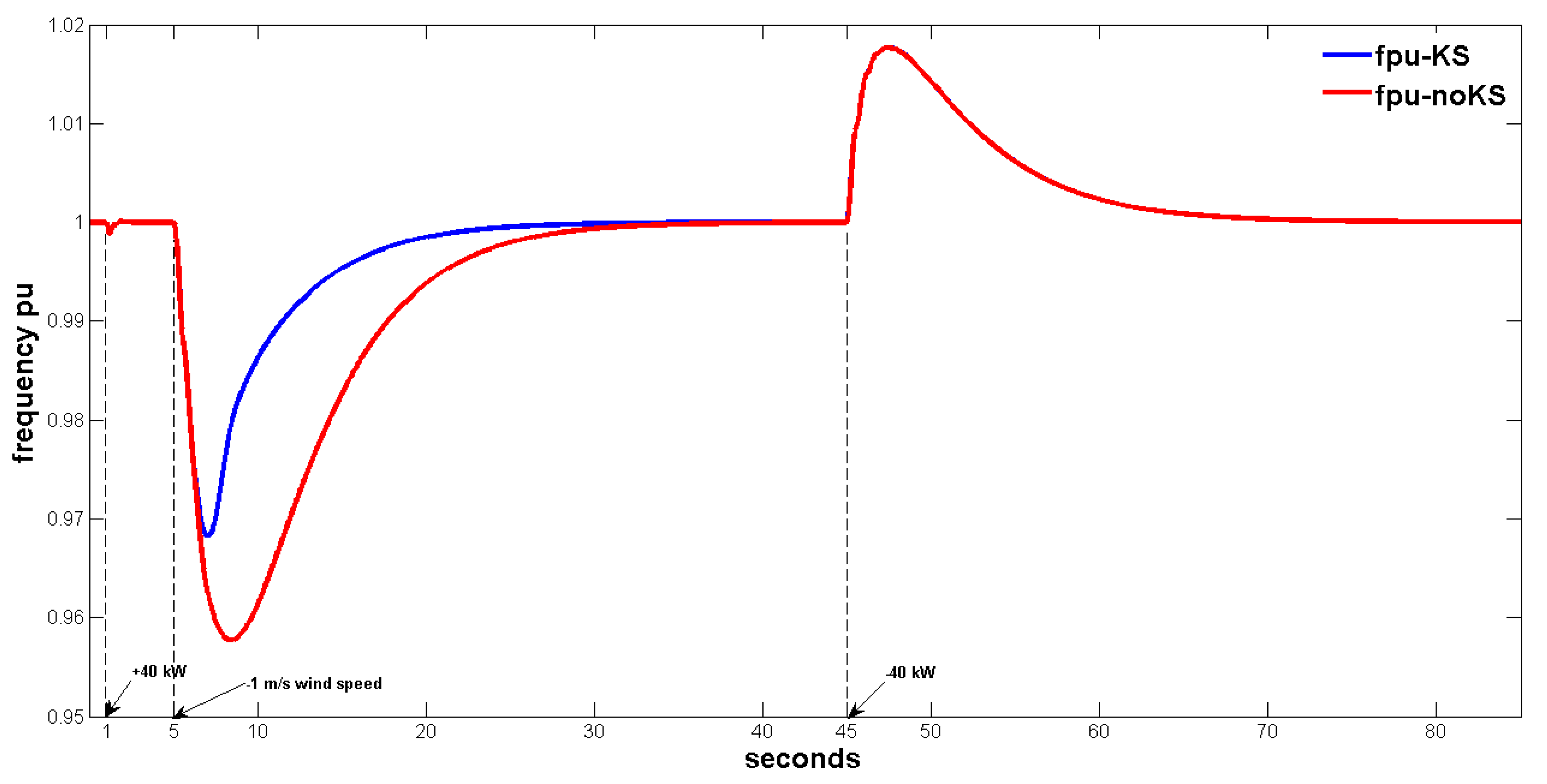
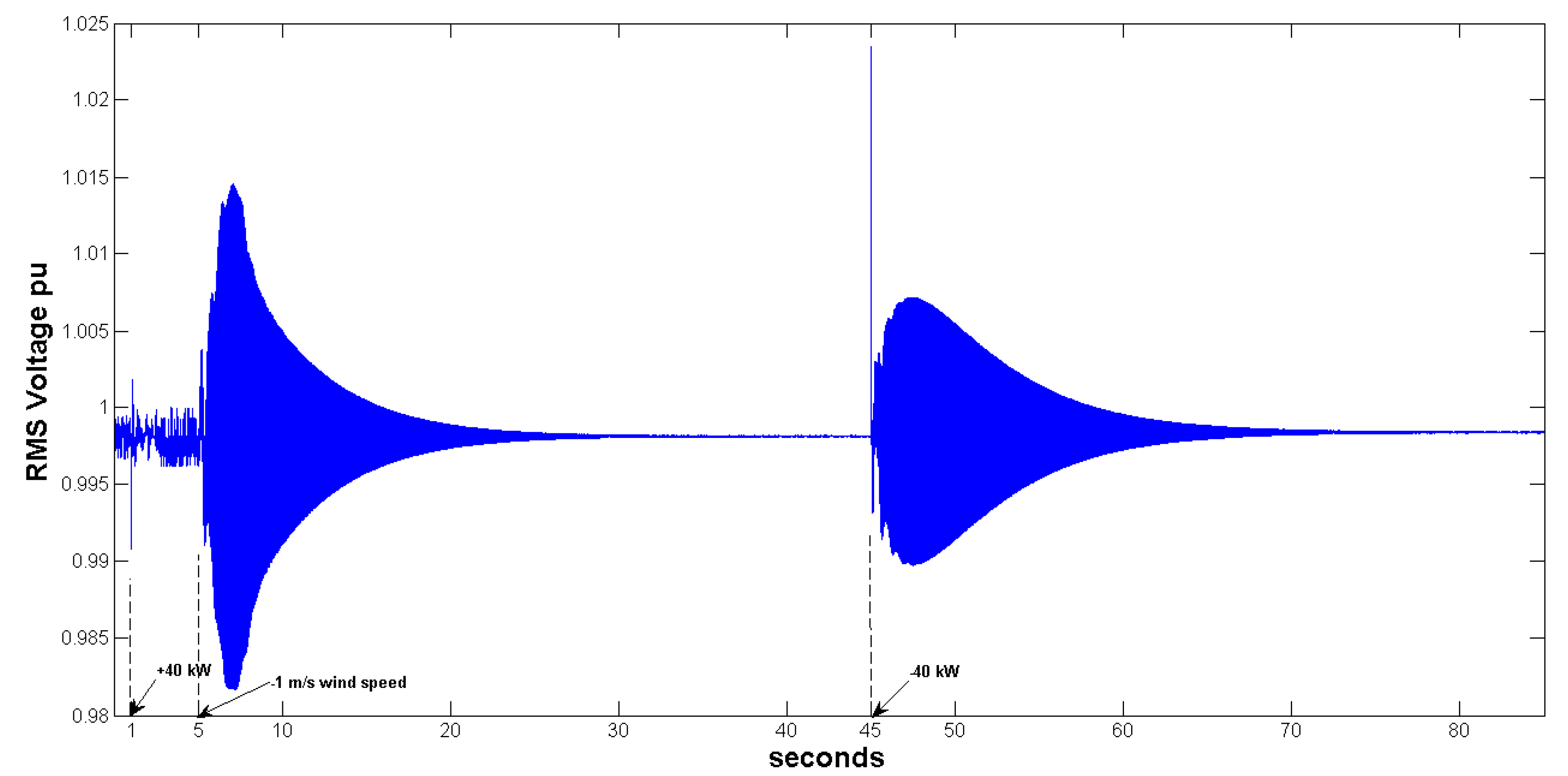
Figure 1. Wind-hydro power system scheme.
Energies 13 05937 g001
Figure 2. Pelton turbine efficiency vs. water flow rate p.u.
Energies 13 05937 g002
Figure 3. Wind-hydro isolated microgrid Simulink schematics.
Energies 13 05937 g003
Figure 4. Hydraulic turbine Simulink schematics.
Energies 13 05937 g004
Figure 5. Hydraulic turbine speed governor Simulink schematics.
Energies 13 05937 g005
Figure 6. Wind turbine mechanical torque calculation.
Energies 13 05937 g006
Figure 7. Dump load control Simulink schematics.
Energies 13 05937 g007
Figure 8. Microgrid frequency in p.u.
Energies 13 05937 g008
Figure 9. Microgrid RMS voltage in p.u.
Energies 13 05937 g009
Figure 10. Active powers in WTG, HTG, consumer load and dump load in kW.
Energies 13 05937 g010
Figure 11. Hydraulic variables.
Energies 13 05937 g011
Table 1. Simulation results summary.
Variable\CaseWOWO2WH KSWO2WH no-KSWH
Δ f[0.9988, 1][0.9683, 1][0.9577, 1][1, 1.0177]
Δ f [%]−0.12−3.17−4.23+1.77
Δ V[0.9908, 1.0018][0.9817, 1.0146][0.9758, 1.0195][0.9898, 1.0235]
Δ V [%]1.13.294.373.37
t s [s]0.97526.48732.844030.892
Publisher’s Note: MDPI stays neutral with regard to jurisdictional claims in published maps and institutional affiliations.

