1. Introduction
The trend in the automotive industry towards electrified powertrains is continuously increasing. A compact drive unit including an electric traction drive, transmission, and power electronics is an established solution. The heat generated in the electric drive is one of the limiting factors in terms of driving performance. Hence, thermal management and the dedicated design of cooling concepts become even more important. Depending on whether a direct or indirect cooling system is used (which refers to the direct or indirect contact of the cooling fluid with the electric drive), there are different requirements of the cooling fluid. Indirect cooling systems allow the usage of cooling fluid that is optimized for heat transfer only as the fluid circulates in isolated cooling channels. Water-/glycol-based fluids are often used in indirect cooling systems as they have excellent thermal conductivity and capacity properties. Whereas in a direct cooling system, the cooling fluid comes into contact with electrical components to transfer the heat more efficiently from the source. Because of a requirement for low electrical conductivity and the preferred usage of existing transmission fluid as a coolant, the direct cooling system needs advanced transmission fluids (ETFs) that combine lubrication and electrical insulation properties.
The fluid needs to combine the conventional requirements defined by the transmission parts with the new requirements coming from the direct cooling concept. One important requirement is heat transfer. Therefore, the thermal conductivity and thermal capacity is a property purely defined by the fluid.
Figure 1a shows how the thermal properties of transmission fluids compare to a conventional water and a water glycol-based coolant. Even if the difference in terms of thermal properties of transmission fluid appears to be relatively low, there are minor differences present; see
Figure 1b. Furthermore, other fluid properties, e.g., viscosity, affect the cooling significantly and need to be considered. The purpose of this work is to assess the cooling effect by considering both fluid properties and heat transfer in a direct cooling system.
The direct inside cooling method is still relatively new and unexplored in the automotive industry. The multiphase flow in the inside of the machine can currently only be evaluated on the test bench or numerical model, which are time-consuming approaches. For the investigation of the fluid, a thermal network model is used, which is validated with measured data of a transmission fluid and can reproduce the interior cooling. In order to evaluate another fluid, an approach is presented in this publication that takes the thermal properties of the fluid into account, and thus allows a direct comparison. Therefore, the heat transfer coefficients are derived using an empirical equation for the model. Subsequently, the effects of the individual material parameters and the influence on the continuous power are presented.
To check for plausibility, the fluid chosen by the model is investigated on a dedicated eMotor cooling (EMC) test evaluating cooling performance and durability behaviour.
2. Cooling Systems for Electrical Machines
To get an overview of the current cooling systems of electrical drives, the following section describes the classification of different concepts. The European standard IEC 60034-1 [
1] differentiates cooling systems for electrical machines as follows:
A distinction is made between passive cooling, cooling driven by the machine itself (self-cooling), and externally applied cooling (external-cooling). A high power density is required in current electrified vehicle bodies. Sufficient heat dissipation cannot be achieved with self-cooling systems.
The application in electric traction drives with external cooling can be divided into three areas.
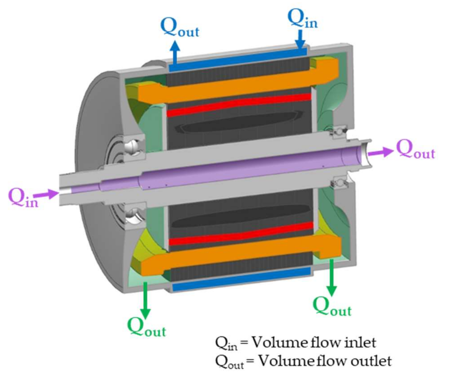
Figure 2 shows an overview of the main cooling systems.
Stator jacket cooling (blue) with water glycol or lubricating fluid;
Rotor shaft cooling (magenta) with water glycol or lubricating fluid;
Interior cooling (green) with lubricating fluid.
The thermal simulation for the interior cooling is difficult to predict because of the fluid/air mixture. In various test bench measurements with different machine types, it has been observed that this heat path has the greatest effect on the cooling performance; for this reason, the fluid evaluations are carried out with this heat sink.
3. Thermal Model for Electrical Machines
The thermal evaluation of electrical machines is often performed using lumped parameter models (LPMs). This type of modeling simply describes the heat sources and sinks as well as the heat transfer between components, and thus quickly provides information regarding the thermal behavior [
2]. The use of LPMs for electrical machines has been discussed by various authors [
3,
4,
5,
6]. These models map the controlled system and can thus quickly generate information on the thermal behaviour. The aim of this modelling is to predict the component temperatures
T as accurately as possible on the basis of various boundary conditions. The system boundaries are stored in the model as thermal nodes, which contain the specific information, such as the heat capacity.
where
H = enthalpy;
Q = heat;
U = internal energy;
p = pressure;
V = volume;
m = mass;
cp = specific heat capacity;
C = heat capacity;
T = temperature;
t = time;
= heat flow.
The equivalent circuit diagram of an example drive shown in
Figure 3 is greatly simplified. This allows all heat sources and flow to be clearly shown. The respective resistances between the thermal nodes are determined based on the material and flow properties as well as the original component geometry. This tool can be used to generate the balance equations and the resistance matrix for this model. The thermal resistances are compared with measured data using an optimization algorithm. Thus, the thermal load of the components and the cooling medium can be simulated in the model under different boundary conditions, such as the voltage level, volume flows of the fluids, flow temperatures, and operating points.
The equivalent circuit diagram in
Figure 3 is greatly simplified and is only intended to show the basic wiring. Depending on the level of detail, the balance spaces can be refined as desired in order to make the temperature differences in the components visible. As the focus of this publication is not on modeling or balancing, it will not be discussed further. The active components represent the heat sources and are connected to the heat sinks by thermal resistances, such as the cooling jacket or the inside air oil. These resistances are divided in the model into heat conduction, contact resistance, and heat transfer resistance. If the thermal properties of the cooling medium in the inside are changed, the heat transfer coefficients—see
Figure 4—have to be adjusted to show the effects on the cooling behavior.
In order to evaluate different oil properties in a thermal model, the heat transfer coefficients can be compared with a series of measurements. As the effort on the test bench is high, this is impossible in most cases. Hence, for the present study, an exponential approach for the nut number was developed. Equation 4 is calculated for two fluids in order to use the ratio from this calculation to adjust the heat transfer parameters in the model. The correction factor b is for the adjustment in the model and is reduced in the case of a comparison [
7].
where
Nu = Nusselt number;
Re = Reynolds number;
Pr = Prandl number;
b = correction factor for heat transfer.
From an internal series of individual tests, the effectiveness for Re >
with m = 0.8, n = 0.6 were determined for a rotating disc, similar to the rotor ends. As no other data are available for the calculation of the other heat transfer coefficients, these parameters were also applied to the other heat transfer surfaces. For a detailed transfer, further investigations must be carried out for all heat transfer surfaces. The correction factor from a reference fluid (ETF1) to a high reference example (HRE) from the
Table 1 is 1.513. The HRE is an imaginable oil with the maximum possible material properties for inside cooling. It is impossible to combine these cooling performances with other lubrication related requirements, which should demonstrate at this stage the influence of the parameter on the cooling.
In order to check the acceptability of the calculated correction factors, a further correction factor was determined using the Colburn analogy [
8]. This has a special validity for turbulent flows in pipes and is thus not the first choice for multiphase flow. A similar comparison is made here as in the approach above. A relation is determined from the heat transfer coefficients. If the velocities in the formula are assumed to be equal, only the Prandl number, density, and heat capacity have an influence on the relation.
where
= fanning friction factor of a smooth pipe;
= density;
= effective velocity outside the boundary layer;
= specific heat capacity;
= heat transfer coefficient.
Calculation with this analogy results in a correction factor of 1.437. Comparison of the correction factors shows a similar increase in the heat transfer coefficients of about 50%.
4. Sensitivity Study of Substance Properties
In order to demonstrate the influence on thermal performance, the first step is to determine which material property has the greatest potential. Because the coolant, in most cases, is also used to lubricate the gearbox and the bearings, only certain fluids can be used. The minimum and maximum limit values for a sensitivity study were agreed upon with industry experts. In order to show the change for continuous performance, one parameter was changed at a time, while all others retain their original values.
Figure 5 shows the torque change compared with the reference fluid as a result of the change of individual material properties. The comparison should show how the individual parameters affect each other. The boundary conditions such as state of charge, limit temperature, and inlet temperature are identical. At first glance, it can be seen that the viscosity shows the greatest deviation. This is also because of the fact that the percentage change versus the reference fluid is the greatest. For the study, only a single volume flow was considered. If this is changed, the deviations to reference will be different. The deviations in this study are as follows:
The percentage deviations depend on both the actual power and the speed, as the losses in the stored map do not show a linear trend. To make the approach visible for a general machine assessment, the effects on continuous power are compared in
Figure 6. All boundary conditions such as state of charge, limit temperature, inlet temperature, and volume flow are identical. The displacement of the continuous power as well as the effect of the material properties on the transported losses is shown. Another fluid was defined for the specified application from the knowledge gained. The target of ETF2 is to improve the cooling ability while maintaining all other requirements of a transmission fluid. A comparison was made of the continuous limit curves with both ETF1 and ETF2 and the maximum high reference values from
Table 1.
When looking at two cooling media in
Figure 6, only a small difference can be seen, as the thermal properties change only slightly. Nevertheless, an improvement of approx. 3% over a wide speed range can be achieved by the choice of fluid. The significance of the material properties can be seen in the comparison of the maximum values. In the stationary case, the medium can significantly increase the continuous performance and shows the performance that can only be achieved by the coolant. Depending on the application and machine dimensions, the percentage change can vary. Nevertheless, the performance can be increased by using a more powerful coolant. This also has an influence on the transient behaviour of the machine and ensures a lower temperature level during cycle runs. Alternatively, a reduction of the overall cooling system is also possible through better material properties. For example, a smaller pump can be used by reducing the volume flow, which also lowers the pressure level and increases the efficiency.
5. Test Setup for the Evaluation of Cooling Transmission Fluids
Based on the previously presented calculation method, the testing of the preselected fluids ETF1 and ETF2 is presented below. Two main objectives for testing are presented in this work. First, testing to prove the advantage determined in the previous section with regards to the cooling effect of ETF2 compared with ETF1. Second, to test the preferred fluid in order to estimate the fluid lifetime performance in an application with an interior cooling concept. For the investigation of these questions, a special test stand, the so-called EMC (eMotor cooling), was developed. Hereinafter, the EMC test setup is presented followed by an outline of the test conditions and discussion of the test results.
Test Setup
The aim of the experimental setup was to estimate the cooling effect of ETF1 and ETF2 against each other, as well as to investigate the thermal stress on the fluid, and thus the aging effects by analyzing the fluids with standardized methods [
9].
To simplify the test complexity and to make it realistic, the test setup was coupled to an external drive. All results presented in this work are conducted at a constant speed of 1000 rpm. To avoid induction resistance from the external drive and to neglect core losses, the permanently excited magnets in the rotor of the permanently excited synchronous machine were demagnetized. The electrical power supply to the coils in the stator was controlled, so that realistic heat development and heat transfer between the coils and the fluid was ensured. The main objective was to reach a maximum temperature at windings of 160 °C or 180 °C. Because of a relatively symmetrical distribution of the individual coils in the rotor, the current feed of the coils was carried out by direct current (DC) power supply. The test setup including the necessary peripherals is outlined in
Figure 7.
The identical fluid distribution in the EMC compared with an eMotor in real operation replicates the heat dissipation under defined conditions and represents the thermal stress on the fluid. Based on the intended field of application and the selected insulation class H according to [
10], the absolute maximum temperature at the windings of 180 °C was defined.
The fluid distribution through the internal rotor cooling is sketched in
Figure 2. Comparable to the intended application, the fluid is guided through the hollow shaft. The hollow shaft contains individual nozzles at two positions of the shaft in the area of the end windings. Owing to the applied overpressure, the fluid from the hollow shaft passes through the nozzles into the interior of the eMotor. The applied rotation distributes the fluid to the windings [
11].
For this work, one single eMotor was used. The main reason for this was to minimize the potential measurement variation of the temperatures by the installed temperature sensors in the stator (16 temperature sensors were used for this work on the stator only). Therefore, a working cleaning procedure of the eMotor is essential. A specially developed flushing procedure (which includes flushing conditions), as well as a dedicated flushing fluid and a repeated change of flushing fluid, provides the intended outcome.
Figure 8 shows a visual comparison of fresh test fluid (a), flushing fluid (b), and end of test fluid as a representative example for ETF1 after 200 h at 160 °C (c) followed by samples after intermediate cleaning steps (d–f). With each flushing step, the color of the samples becomes closer to the original color of the flushing fluid. Thus, the flushing success can be visually assessed. In addition, the visual assessment was confirmed by chemical analysis by applying Fourier transform infrared spectroscopy (FTIR).
6. Test Results and Discussion
A general presentation of the test stand, the individual test procedure, and the obtained results is discussed below.
6.1. Thermal Performance of Selected Fluids
The cooling benefit of ETF2 compared with ETF1 determined in
Figure 6 is experimentally investigated on EMC and presented in this section.
The purpose of this work is not to measure the absolute heat transfer. The focus of this work is to carry out a relative rating of the heat transfer between the ETF1 and ETF2. The relative rating of heat transfer was done using the installed temperature sensors in the windings. The schematic position of temperature sensors is shown in
Figure 9.
Eight temperature sensors are installed on each side of the coil ends, with two sensors located each at 90° (starting at the top position of the stator), leading to a total of 16 temperature sensors for both sides. A hypothetical comparison of two fluids with identical heat input , but detecting a temperature difference (measured directly on the heat windings), must show that the fluids transfer the heat differently. The potential different heat losses due to different heat radiation are negated because of similar test conditions. In the comparison of the two fluids, the fluid with higher temperatures (measured) indicates poorer heat transport. This allows conclusions regarding heat transfer properties to be drawn from the measured temperatures.
Even if an absolute assessment of the heat transfer is not readily possible, a relative comparison of the fluids can be made based on the temperature comparison. Analogous to the comparative assessment of the torque in
Figure 6, the comparison in this section is based on measured temperatures.
To allow comparison to the results presented in
Figure 6, the measurements below are carried out at a flow rate of 3 L/min. The mechanical losses, mainly occurring at bearing and sealings, were recorded, but repeal as the power loss of both fluids is identical.
Figure 10 shows the temperature difference of ETF2 compared with ETF1 for each installed temperature sensor in the stator shown in percent at identical power
W.
It was observed that all sensors show the same trend. Based on the measured temperatures with the ETF1, an average improvement of 1.5% of heat transfer was recorded with ETF2. The sensor and thus position-dependent differences, shown in
Figure 10, are design-dependent and are not discussed in this work, but offer additional information for the design of the electric machine.
The relative comparison of the fluids based on the measured temperature confirms the calculated trend as presented above; see
Figure 6. ETF2 is the favored fluid from the cooling performance, but the usage of the fluid as a coolant leads to potential further demands. Fluid aging due to continuous heat transfer and operating conditions at extremely high temperature with up to 180 °C is discussed in the next section.
6.2. Aging of Electrified Transmission Fluid when Used as a Coolant
The usage of a transmission fluid as a coolant results in several additional requirements of the fluid. As there is hardly any field experience in the automotive industry, various committees, e.g., Deutsche Institut für Normung (DIN), Forschungsvereinigung Antriebstechnik (FVA), Deutsche Wissenschaftliche Gesellschaft für Erdöl, Erdgas und Kohle (DGMK), are in the process of defining the necessary requirements for fluids and specifying them by means of specification requirements. A few papers have already been published on the subject [
12,
13,
14,
15,
16]. Additional tests are desired to detect potential issues as early as possible especially if uncertainty is high. In the scope of this work, accelerated tests were carried out under extreme operating conditions and different fluid properties at the start and end of test (EOT) were used to rate the aging effect. A relatively small property change forecasts stable long-term usage and low fluid aging. Nevertheless, it should be noted that any pre- or post-comparisons ignore interim changes. This means that potentially opposite effects with unstable behaviour remain undetected.
In several applications with eMotors, temperatures of up to 180 °C are considered. Such a high temperature usually occurs only in some local areas at the coils and just for a relatively short time. Aiming for an application-oriented investigation, the target of this work is to mimic realistic conditions in the specially developed EMC rig and avoid unrealistic thermal stress and fluid changes by aging mechanisms when considering the maximum operating temperatures and conditions.
Compared with the previous section, where a constant heat input energy was used, the test procedure for the investigation of thermal stress was fundamentally changed. In order to be able to adjust the maximum temperature, the quantity of heat energy is used as a control parameter. The maximum temperature of 1 of the 16 installed temperature sensors was defined as the input variable in the control loop. This control setup ensures that the maximum thermal stress is accounted for without exceeding local temperature limits and avoids damaging the hardware.
In principle, the maximum temperature can be defined as the target variable. The investigation was carried out with a defined maximum temperature of 160 °C and 180 °C. Derived from the desired operating strategy in the application, the accumulated operating time at 160 °C was defined as 200 h and at 180 °C as 80 h in continuous operation. As a further relevant condition for the application, the fluid inlet temperature at the hollow shaft was investigated at 70 °C and 115 °C.
For all combinations of maximum temperature and inlet temperature investigated, the samples were assessed after the EMC tests relative to the fresh fluid. Without presenting single test results, the laboratory tests showed practically no change in fluid properties. No increase in viscosity or total acid number (TAN) was observed, which would indicate chemical fluid aging. Elemental analysis of the fluid confirmed the stable behavior. Only boron content dropped slightly, but it remained in a typical order of magnitude compared with other gearbox tests and does not represent an unusual finding at this point. The copper content in the fluid was below the detection limit [
9]. The thermal properties of the fluid showed no change.
Figure 11 shows electrical volume resistivity changes from end of test samples compared with fresh fluid samples. Without considering the corresponding test conditions of the EMC test in detail, all samples tested show a clear increase in the electrical volume resistivity.
The increased resistivity after the EMC test, and thus after fluid aging, is opposite to the established expectation in the industry, which is usually explained by two approaches. On the one hand, oxidation leads to more polar components in the fluid, which increase the conductivity or reduce the resistance of the fluid. On the other hand, contamination might occur, e.g., abrasive particles or water, which may also increase the conductivity.
The measured increase in resistance after EMC indicates that the conductivity is also influenced by other parameters and the previous explanatory hypotheses must be supplemented by further considerations. As the chemical analysis of the EOT samples does not show any abnormalities, the potential influence of contamination is most likely very low. It is assumed that the evaporation of short-chain and polar components of the fluid prevails and leads to superimposed effects to an increased resistivity. This highlights how essential it is to use realistic conditions for aging. Excessive thermal and oxidative stress in established laboratory tests or too severe test bench tests can lead to incorrect conclusions.
In addition to the chemical analysis of the fluid samples, a visual rating of the stator in general, and especially the coil end, was carried out at regular intervals. The assessment took place without disassembling the eMotor housing. Except for slight discoloration of the binding threads, the coated coil wires and the resins showed no porosity or cracking; see
Figure 12. No black copper sulfide deposits were found that could lead to conductive layers.
7. Conclusions
In order to optimize installation space, but also to increase the efficiency and performance of electric drives, the development goal is a smaller and lighter eMotor. Heat dissipation is an increasing challenge, particularly in the case of a drive with small size. New cooling concepts in which the transmission fluid is also used as a coolant of the eMotor are becoming increasingly important in the automotive industry. In principle, different concepts are possible, but the interior cooling concept is one of the most effective, explaining the focus of this work. The fluid is in direct contact with the coil ends, and then absorbs the heat and dissipates it. This results in thermal requirements of the fluid, which must be considered in addition to the existing requirements coming from transmission components. The heat dissipation, as well as the thermal aging of the fluid and compatibility with new materials, must be defined.
To assess the heat dissipation of fluids in the complex environment of an eMotor, a resistance-based model was developed and checked for plausibility using the Colburn analogy. The calculation model is the basis for the subsequent sensitivity study with the aim to define the relevant fluid parameters describing heat dissipation. Based on the knowledge gained, two ETFs (ETF1 and ETF2) were selected for further investigation and compared with the model in terms of heat dissipation. Based on the model, the ETF2 showed an improved heat dissipation of approximately 3% against ETF1 over a wide speed range. In order to validate the calculation model, a special eMotor cooling (EMC) test was developed. Both ETFs were tested in EMC for heat dissipation. The better cooling effect of ETF2 compared with ETF1 is observed in the model-based comparison as well as experimentally with the EMC rig.
For the investigation of thermal aging, a test matrix on the EMC rig with maximum temperatures of 160° and 180 °C was defined. The results of ETF2, as the fluid with the better cooling performance, are presented in the scope of this work. Both analytical analysis of the fluid samples and the visual rating of the electric drive components show a stable behaviour over time. The electrical properties of the fluid showed an improved insulating effect at the end of the durability tests.
Author Contributions
All authors have read and agreed to the published version of the manuscript. R.L. Data curation, formal analysis, methodology, resources, validation, visualization, writing original draft, writing of review and editing. A.P. Data curation, resources, validation, visualization, writing original draft, writing of review and editing. M.M. Formal analysis, methodology, software. M.K. Methodology, software. C.W. Funding acquisition, project administration, resources. F.G. Supervision.
Funding
This research received no external funding. We acknowledge support by the KIT-Publication Fund of the Karlsruhe Institute of Technology.
Conflicts of Interest
The authors declare no conflict of interest.
References
- IEC 60034-1: Rotating Electrical Machines; VDE-Verlag: Berlin, Germany, 2017.
- Oechslen, S. Thermische Modellierung Elektrischer Hochleistungsantriebe. Ph.D. Thesis, University of Stuttgart, Stuttgart, Germany, June 2018. [Google Scholar]
- Huger, D.; Gerling, D. An advanced lifetime prediction method for permanent magnet synchronous machines. In Proceedings of the 2014 International Conference on Electrical Machines (ICEM), Berlin, Germany, 2–5 September 2014; pp. 686–691. [Google Scholar]
- Nategh, S.; Huang, Z.; Krings, A.; Wallmark, O.; Leksell, M. Thermal modeling of directly cooled electric machines using lumped parameter and limited CFD analysis. IEEE Trans. Energy Convers. 2013, 28, 979–990. [Google Scholar] [CrossRef]
- Liu, Z.; Howe, D.; Mellor, P.; Jenkins, M. Thermal analysis of permanent magnet machines. In Proceedings of the Sixth International Conference on Electrical Machines and Drives, Oxford, UK, 8–10 September 1993; pp. 359–364. [Google Scholar]
- Qi, F.; Schenk, M.; De Doncker, R. Discussing details of lumped parameter thermal modeling in electrical machines. In Proceedings of the 7th IET International Conference on Power Electronics, Machines and Drives (PEMD 2014), Manchester, UK, 8–10 April 2014; pp. 1–6. [Google Scholar]
- Thoma, A. Reduzierung der Luftreibungsverluste und Temperaturen in Schnelldrehenden Motorspindeleinheiten. Diploma Thesis, University of Technology Darmstadt, Darmstadt, Germany, June 1995. [Google Scholar]
- Lechmann, A. Modellierung von Wärmeübertragern in den Gaswechselsystemen von Verbrennungsmotoren. Ph.D. Thesis, Technical University of Berlin, Berlin, Germany, July 2008. [Google Scholar]
- ASTM D5158-18. Standard Test Method for Multielement Determination of Used and Unused Lubricating Oils and Base Oils by Inductively Coupled Plasma Atomic Emission Spectrometry (ICP-AES); ASTM: West Conshohocken, PA, USA, 2018. [Google Scholar]
- DIN EN 60085. Electrical Insulation—Thermal Evaluation and Designation; Deutsches Institut für Normung; VDE Verlag GmbH: Berlin, Germany, 2008. [Google Scholar]
- Beck, C. Modeling of multiphase flow in electrical motors. In FVA E-Motive Expert Forum on Electric Vehicle Drives and E-Mobility; Forschungsvereinigung Antriebstechnik e.V.: Schweinfurt, Germany, 2019. [Google Scholar]
- Speed4E Board. Hyper-High-Speed for Electric Vehicles to Achieve Maximum Ranges. Available online: http://www.speed4e.de/Joomla/index.php/en/ (accessed on 9 November 2020).
- Dobrowolski, C. Low Viscosity lubricants for electrified transmission concepts. In Proceedings of the GETLUB Conference, Hamburg, Germany, 6–7 November 2018. [Google Scholar]
- Petuchow, A.; Plaatje, A.; Maelger, H. Use of existing and new AT and DCT fluid technology in hybrid transmission designs as a coolant. In FVA E-MOTIVE Expert Forum Electric Vehicle Drives; Forschungsvereinigung Antriebstechnik e.V.: Schweinfurt, Germany, 2019. [Google Scholar]
- Lotfi, B. Ultra-Low Viscosity Synthetic e-DF; How Synthetic Base Oils Can Help Novel Formulation for e-Mobility Fluids. In Proceedings of the 18th International Congress and Expo, CTI Symposium. Berlin, Germany, 9–12 December 2019. [Google Scholar]
- Maelger, H.; Petuchow, A.; Plaatje, A.; Yungwan, K.; Banks, A. Realistic testing to assess how electrified transmission fluids will withstand ageing. In Proceedings of the 18th International Congress and Expo, CTI Symposium, Berlin, Germany, 9–12 December 2019. [Google Scholar]
Figure 1.
This diagram shows the thermal material properties of (a) electrical transmission fluids (ETF) and a water glycol coolant at 100 °C in comparison with water at 20 °C; (b) transmission fluids shown in detail.
Figure 1.
This diagram shows the thermal material properties of (a) electrical transmission fluids (ETF) and a water glycol coolant at 100 °C in comparison with water at 20 °C; (b) transmission fluids shown in detail.
Figure 2.
Schematic of possible cooling systems for electrical machines.
Figure 2.
Schematic of possible cooling systems for electrical machines.
Figure 3.
Thermal model with the resistances between the active components and the cooling medium using the example of an induction machine.
Figure 3.
Thermal model with the resistances between the active components and the cooling medium using the example of an induction machine.
Figure 4.
Heat transfer coefficient areas of the machine using the example of an induction machine.
Figure 4.
Heat transfer coefficient areas of the machine using the example of an induction machine.
Figure 5.
Effect of material properties on the thermal behaviour of the electrical machine.
Figure 5.
Effect of material properties on the thermal behaviour of the electrical machine.
Figure 6.
This figure shows the effect of the cooling medium for the electrical machine, for two electrical transmission fluids (ETF1 and ETF2), and for the maximum possible values (a) and continuous limit (b) percentage change of the torque to the reference ETF1.
Figure 6.
This figure shows the effect of the cooling medium for the electrical machine, for two electrical transmission fluids (ETF1 and ETF2), and for the maximum possible values (a) and continuous limit (b) percentage change of the torque to the reference ETF1.
Figure 7.
Schematic test setup of the electro motor cooling (EMC) test rig. DC, direct current.
Figure 7.
Schematic test setup of the electro motor cooling (EMC) test rig. DC, direct current.
Figure 8.
Fluid samples as a visual comparison of (a) fresh test fluid ETF1, (b) fresh flushing fluid, (c) representative example for ETF1 end of test sample, (d) sample after first flushing step, (e) sample after second flushing step, and (f) sample after third flushing step.
Figure 8.
Fluid samples as a visual comparison of (a) fresh test fluid ETF1, (b) fresh flushing fluid, (c) representative example for ETF1 end of test sample, (d) sample after first flushing step, (e) sample after second flushing step, and (f) sample after third flushing step.
Figure 9.
Schematic position of temperature sensors installed in the coil end of the used eMotor.
Figure 9.
Schematic position of temperature sensors installed in the coil end of the used eMotor.
Figure 10.
Temperature difference of ETF2 compared with ETF1 in percent relating to the measured temperature on each temperature sensor installed on the stator.
Figure 10.
Temperature difference of ETF2 compared with ETF1 in percent relating to the measured temperature on each temperature sensor installed on the stator.
Figure 11.
Electrical volume resistivity changes end of test samples compared with fresh fluid samples. Measured according to DIN EN 60247, @ 90 °C @ 250 V/mm.
Figure 11.
Electrical volume resistivity changes end of test samples compared with fresh fluid samples. Measured according to DIN EN 60247, @ 90 °C @ 250 V/mm.
Figure 12.
Example picture of the coil end (a) coil before test; (b) and (c) the conditions of the coils after the first test at 180 °C for 80 h; and (d) coil conditions after the last test used for this work including several tests at 180 °C and 160 °C.
Figure 12.
Example picture of the coil end (a) coil before test; (b) and (c) the conditions of the coils after the first test at 180 °C for 80 h; and (d) coil conditions after the last test used for this work including several tests at 180 °C and 160 °C.
Table 1.
The table shows the thermally decisive material properties of the reference fluid (ETF1) in the model and a high reference example (HRE) with maximum possible values measured at 80 °C.
Table 1.
The table shows the thermally decisive material properties of the reference fluid (ETF1) in the model and a high reference example (HRE) with maximum possible values measured at 80 °C.
| Material Properties | ETF1 | HRE |
|---|
Density
| 808 | 820 |
kin. Viscosity
| | |
spec. Heat Capacity
| 2120 | 2380 |
Thermal Conductivity
| 0.132 | 0.15 |
| Publisher’s Note: MDPI stays neutral with regard to jurisdictional claims in published maps and institutional affiliations. |
© 2020 by the authors. Licensee MDPI, Basel, Switzerland. This article is an open access article distributed under the terms and conditions of the Creative Commons Attribution (CC BY) license (http://creativecommons.org/licenses/by/4.0/).

 ,
, 


