Abstract
This paper presents an analysis of the accelerometer input–output energy distribution based on the upper bound of the absolute dynamic error (UBADE). This analysis corresponds to the input and output accelerometer signals, determined previously by mathematical modeling. Obtained results may provide the basis for verifying the correctness of the algorithms intended for the determination of the UBADE.
1. Introduction
In the field of theory and practice related to accelerometers, as for the other types of measurement sensors, there are known test procedures used for calibration [1,2,3,4,5]. This type of measurement experiment usually consists of determining the time or frequency responses of such sensors [1,2,4]. On the basis of these responses, the selected parameters of the sensors are determined [2], which are then compared with their equivalents declared by the manufacturer in the corresponding datasheet. For accelerometers, the calibration process usually determines voltage sensitivities [2,4]. This parameter is determined based on a measurement of one frequency response (amplitude) or the simultaneous measurement of two frequency responses (amplitude and phase) [6,7,8,9].
Accelerometers are widely used in the power industry to continuously monitoring the operation of the kinetic system components of turbines used in wind and hydro plants [10,11,12] as well as in the case of drilling platforms [13,14]. Such monitoring is aimed at current determination of the technical condition of such components and early diagnosis of all kinds of potential failures. It is very important due to the significant costs associated with the removal of the effects of failure of turbine components used in various types of power plants [15]. Therefore, it seems justified to select an appropriate type of accelerometer with a specific accuracy of the processing of measurement signals. Such accuracy can be achieved through the use of the appropriate procedures dedicated to determining of the errors of accelerometer processing [16,17,18,19], which can only ensure their mutual comparability.
For accelerometers with the same operating range but from different manufacturers, there are no clear criteria for mutual comparisons of the accuracy of measurement signal processing [4,5]. This is due to the obvious fact that for all instruments intended for measuring quantities that vary over time (dynamic), there is no accuracy class, such as in the case of instruments intended for measuring constant quantities (static). However, mutual comparability among accelerometers can be achieved by using procedures for determining the upper bound of the dynamic error (UBDE) [16,17,18,19]. Taking into account that the value of the dynamic error [20,21,22,23,24,25] and the dynamic properties of the accelerometer are also influenced by the shape of the input signal [16,17], to determine the UBDE, it is necessary to obtain the critical case for such a signal [16,17]. This signal is constrained in its magnitude and rate of change [26,27] and is determined via mathematical modeling [16,17]. The constraint of the magnitude is related to the measuring range of the accelerometer, while the constraint of the rate of change is due to its dynamics (dynamic properties) [16,17]. To determine the UBDE, it is necessary to apply the selected comparative quality criterion. In the measuring technique, the most popular criteria are integral-square error and absolute error [16,17]. The solutions presented in this paper apply to the absolute error criterion, and its possible highest value is defined as the upper bound of the absolute dynamic error (UBADE).
The algorithm for determining the UBADE has been mathematically advanced to a great extent [17,28]. Hence, its implementation in the selected programming environment may, in many cases, present significant difficulties [28]. Therefore, it seems necessary to develop procedures enabling the verification of both the implemented computer program for UBADE determination and the input signal with constraints related to this signal. Considering the above, this paper proposes a procedure based on an analysis of the energy [29,30,31,32,33,34,35,36] of the accelerometer’s input and output signals, obtained by mathematical modeling [37,38], for which the UBADE is determined.
The first approach to analyze the energy of signals producing the UBADE is presented in the paper [29]. However, it concerned only the application of a short-time Fourier transform (STFT) with excluding of analysis of the energy distribution for the above signals. The next examples of research are presented in the paper [30] and they relate to the energy distribution determination, but in the case of the analysis of signals maximizing the integral square error. The solutions presented in this paper are obtained by applying both the genetic algorithm and the wavelet analysis. A similar study is presented in the paper [31]. However, they concern of the case of the input signals constrained only in its magnitude.
It was assumed that the conducted analysis would allow us to verify the correct implementation of the algorithms dedicated to UBADE determination. This verification ensures that the accelerometer accuracy analysis based on UBADE can be reliable. This is extremely important, as a high accuracy of accelerometers is very desirable from an engineering point of view. This verification can also ensure the reliability of the mutual comparability of the different types of accelerometers.
The accuracy of the analysis presented in this paper may be affected by the uncertainties associated with the accelerometer parameters obtained as a result of identification. The results of research in this area are presented and discussed in detail in the papers [28,39]. The influence of the noise on the accuracy of the input–output energy distribution analysis is not considered in this paper. The procedure presented in this paper can be used without any limitation for all types and characteristics of accelerometers.
Section 2 discusses the mathematical formulae leading to the determination of the mathematical model (transfer function) of the accelerometer and the formulae that join the three main parameters of the accelerometer with its cut-off frequency. Section 3 presents the main assumptions for the procedure of the UBADE determination and the basic properties related to the accelerometer input and output signals, which are determined by employing mathematical modeling. Based on the guidelines included in the previous section, Section 4 details the procedure for determining the UBADE when signals with two simultaneous constraints are imposed on the magnitude and rate of change. The analysis is performed for three sets of accelerometer parameters give the most characteristic results. In turn, Section 5 presents an analysis of the input–output energy distribution for three sets of accelerometer parameters. Graphical analyses are shown for each case, together with related conclusions, and a scalogram was used for these analyses as a tool for time–frequency signal decomposition. The final section entitled “Conclusions” summarizes the results obtained in this paper.
2. Theoretical Background
The mechanical construction of the accelerometer is shown in Figure 1 [40,41]. Formulas referring to the mathematical model of accelerometer are described in the previous authors papers [30,31,34,39].
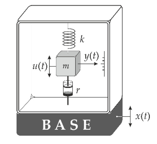
Figure 1.
Mechanical construction of the accelerometer.
The percentage tolerance of the accelerometer voltage sensitivity for frequency equal to the cut-off frequency [Hz] is represented by the following formula:
which is obtained based on amplitude response, where and while and denote natural undamped frequency and damping factor (dimensionless), respectively.
Both the cut-off frequency and tolerance are provided by the accelerometer datasheet.
By expanding Equation (1), we obtain
Based on Equation (2), we can easily obtain when the parameters , and are given.
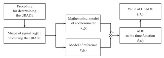
Figure 2.
Block diagram of the methodology for determining the upper bound of the absolute dynamic error (UBADE).
The basis for determining the UBADE is the mathematical model of an accelerometer. This mathematical model is represented by the accelerometer transfer function [30,34,39]. The parameters included in this function are obtained as the results of the accelerometer’s parametric identification [6,7,8,9].
For the modeling purposes in this paper, the accelerometer is assumed to be a low pass system. Additionally, the values of the accelerometer parameters were assumed in advance for the purposes of the analysis. Several sets of accelerometer parameters were analyzed. Of course, the procedure presented here can also be used for real data obtained based on parametric identification.
The value of UBADE is determined based on [16]. A high-order low-pass analog filter with a cut-off frequency corresponding to the frequency band of the accelerometer is used as a reference [42,43]. Use of this reference ensures that the analysis of the UBADE concerns only the frequency range of the accelerometer. For the purposes of this paper, an analog Butterworth filter of the 10th order with the transfer function denoted as was adopted.
The procedure for determining the UBADE was carried out based on the mathematical models and The procedure for the UBADE determination is discussed in detail in Section 4.
This procedure obtains the two-constrained shapes of signal that produce the UBADE. These constraints apply simultaneously to the magnitude and the rate of charge of signal . The second constraint is derived from
where is the time of accelerometer testing, and is the impulse response of the accelerometer, which is determined based on the relation,
where denotes the inverse Laplace transform [16,17].
Figure 3 shows an example signal with two constraints and five time switchings denoted by The magnitude constraints are denoted by (positive constraint) and (negative constraint), while the rate of change constraints are denoted by (signal increase) and (signal decrease) [16,17].
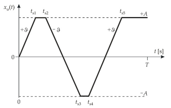
Figure 3.
Example signal with two constraints.
Signal producing the UBADE has properties such that any signal contained in its constraints can only produce the lower value of ADE.
The function presents the ADE for The maximum value of the function can be obtained for time Then, this function is denoted as Figure 4 shows an example function The UBADE is obtained for
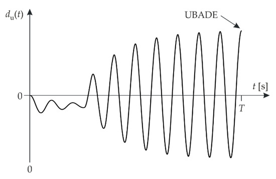
Figure 4.
Example function .
The value of UBADE determined for accelerometers with the same operating range (frequency band) but produced by different manufacturers may provide the basis for their mutual comparability in terms of signal processing accuracy. Thus, an analogy can be found here with the accuracy class of the measuring instruments intended for measuring the constant quantities over time. It should be clearly emphasized that there is no accuracy class for instruments (sensors) intended for measuring the dynamic quantities (variables over time) [5,16]. Hence, the analysis presented in this paper is justified.
3. Procedure for Determining the UBADE
When the input signal is constrained in both its magnitude and rate of change the signal producing the UBADE ( is determined indirectly, as follows:
where is the quantization step of time , which is the duration time of accelerometer testing [16,17,28].
Based on the signal and the impulse response , we can easily determine the error by using the following formula [16,17]:
The impulse response is obtained as the difference
where is the impulse response of the reference. This response is calculated based on the following formula
Equations (16) and (17) in their digital form are [17]
and
where .
The function is obtained in several steps used for transforming the impulse response as follows [16,17,28]:
- Determine the pulse function whose duration is equal to , according to the following equation:
An example function is shown in Figure 5. This function was obtained for the following accelerometer parameters: Hz, , and kHz.
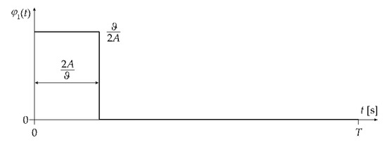
Figure 5.
Example pulse function .
This is the typical shape of this function for any accelerometer analysis. Only the pulse width of is changed. Example figures for the subsequent stages of the procedure for determining the upper bound of the absolute dynamic error were also obtained for the above accelerometer parameters.
- 2.
- Calculate the convolution integral based on the function and the impulse response :
Figure 6 shows the shape of the function , which is typical for any accelerometer parameters.
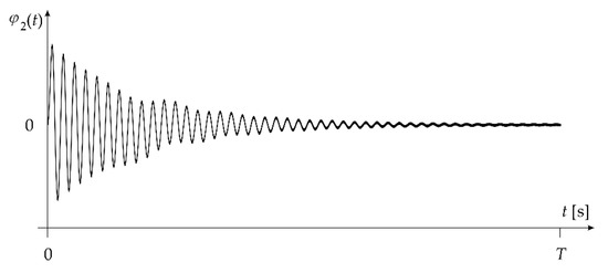
Figure 6.
Convolution integral .
- 3.
- Determine the rectangular function based on the following formula (Figure 7):
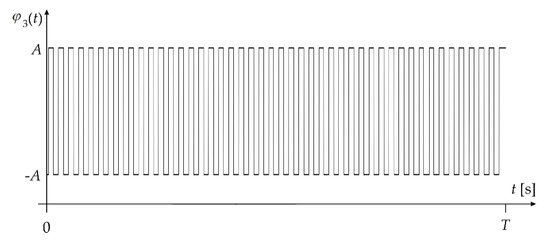 Figure 7. Rectangular function .
- 4.
- Determine the function with value in the first interval and the values or 0 at the other intervals (Figure 8):
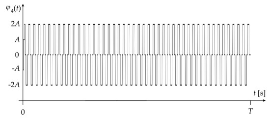 Figure 8. Shape of function .
- 5.
- Determine the function with the following values: 0, , or (Figure 9):
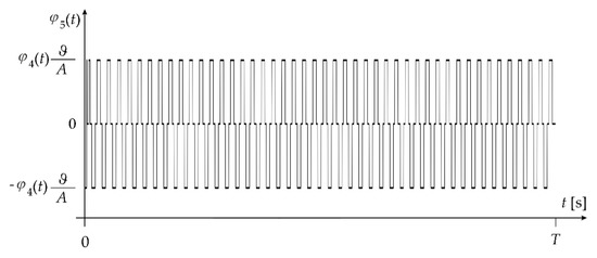 Figure 9. Shape of function .
- 6.
- Determine the signal with two constraints by substituting for in Equation (5) (Figure 10). This signal produces the upper bound of the absolute dynamic error.
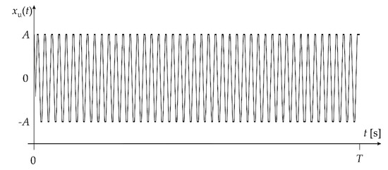 Figure 10. Signal with two constraints.
- 7.
- Determine the absolute error as the time function:
Finally, based on Equation (16), we can easily obtain the upper bound of the absolute error by using the following formula:
which corresponds to Equations (6) and (10).
4. Analysis of the Accelerometer Input–Output Energy Distribution
Next, we present the procedure for analyzing the input–output energy distribution for the three selected sets of parameters included in the mathematical model of the accelerometer. This analysis relates to the input signal and the related output signal and allows an assesment of the frequency components included in these signals. Thanks to this analysis, it may be possible to assess the correctness of the implementation of procedures dedicated to UBADE determination.
The analysis of the input–output energy distribution uses a scalogram that employs both the wavelet method and MATLAB software (R22a, MathWorks, Natick, MA, USA). The scalogram procedure is based on the following formula:
where is the complex conjugate of the wavelet used for the analysis [30,44,45,46], for which a Morlet wavelet (Version, Manufacturer/Company, City, State Abbr. if USA or Canada, Country) was used.
Three sets of accelerometer parameter values for the analysis are tabulated in Table 1. These values were selected from among many other sets as they provide the most characteristic results for the analysis. For all checked cases, a voltage sensitivity equal to was assumed. The tests were carried out for a constant value () of the accelerometer operating band. It was also assumed that the magnitude constraint is equal to the accelerometer’ voltage sensitivity (). The value of frequency was calculated with Equation (2), while the rate of change constraint was calculated via Equation (3). The time of accelerometer testing corresponds to a steady-state of the impulse response

Table 1.
Values of the accelerometer parameters for analysis.
Figure 11 shows the signals and obtained for the accelerometer parameters included in the first row of Table 1. The value of UBADE () is equal to 27.15 Vs.
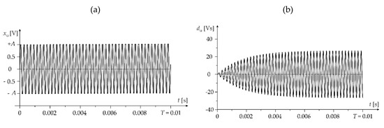
Figure 11.
Input–output relations for energy decomposition (). (a) Signal ; (b) Signal .
Figure 12 presents the results of the analysis of energy distribution carried out for signals and , as shown in Figure 11. This analysis indicates that the dominant frequency component in the signal is only one frequency, The greatest concentration of the input energy occurs around time equal to 2 s, 6 s, and 10 s. This results in a uniform energy distribution in the time domain. In relation to the output signal , frequency is also the dominant component. The greatest concentration of energy occurs for time t ranging from about 5 s and 9 In this case, the energy distribution in the time domain cannot be considered uniform.
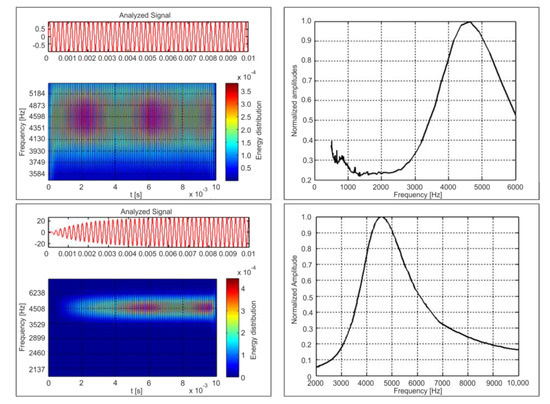
Figure 12.
Scalogram and normalized amplitudes vs. frequency for signals (top plots) and (bottom plots) shown in Figure 11.
Figure 13 shows the signals and obtained for the accelerometer parameters from the second row in Table 1 (). The value of UBADE () is equal to 21.16 Vs. The signal , as in the previous case, has a trapezoidal shape. The signal is similar in shape to the signal determined for , but its phase is inverted.
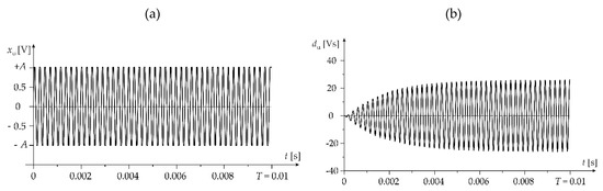
Figure 13.
Input–output relations for energy decomposition (). (a) Signal ; (b) Signal .
Figure 14 presents the results of the analysis for the signals and (Figure 13). The analysis carried out for the signal shows that, apart from the dominant frequency component with a value equal to the frequency the second dominant component with a frequency is visible. The greatest concentration of energy for the signal occurs for time with the ranges of 0 s, 3 s, and 8 s. Non-uniform energy distribution over time is visible in this case. For the signal , the dominant frequency is only The greatest concentration of energy for the signal occurs for time with the ranges of 4 s and 8 s. The energy distribution in this case is more irregular than that in the case where
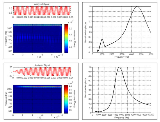
Figure 14.
Scalogram and normalized amplitudes vs. frequency for signals (top plots) and (bottom plots) shown in Figure 13.
Figure 15 shows the signals and for The value of UBADE () is equal to 17.60 Vs. In this case, the signal has a trapezoidal or triangular shape. The signal’s triangular shape means that it has not reached the magnitude constraint.
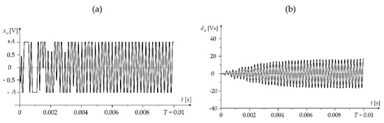
Figure 15.
Input–output relations for energy decomposition (). (a) Signal ; (b) Signal .
Figure 16 shows the analysis of the signals and (Figure 15). Signal contains two dominant frequency components: and Compared to the case of , the component with a frequency equal to shows higher dominance. Analysis of the energy distribution for the signal is divided into two stages: The first one occurs around frequency (left panel), while the second one is around frequency (right panel). The left panel shows the energy concentration for time in the range of 0–2 s. The greatest energy concentration for frequency (right panel) occurs for time in the ranges of 3–6 s and 8–10 s.
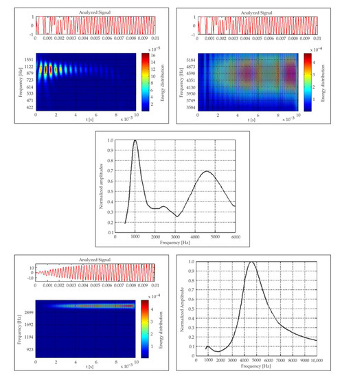
Figure 16.
Scalogram and normalized amplitudes vs. frequency for signals (three top plots) and (two bottom plots) shown in Figure 15.
Additional tests were performed for a damping factor equal to 0.1, 0.2, 0.3, and 0.4. With an increase of this factor, analysis of the signal shows a decrease in the normalized amplitude for the frequency The normalized amplitude for is equal to 0.33. The normalized amplitude for frequency has a constant value equal to 1. Considering the frequency for all the above-mentioned values of the factor , the uniform energy distribution for time in the range of 0–7 s is visible. On the other hand, for frequency , the energy distribution is narrowed to time in the range of 9–10 s. Analysis of the signal for the damping factor equal to 0.1, 0.2, 0.3, and 0.4 shows that with an increase in the value of this factor, there is an increase in the normalized amplitude of frequency For the value of this amplitude is 0.65, while the energy distribution for frequency is uniform for time with a range of 0–7 s. On the other hand, for frequency just as for signal the energy distribution is narrowed to time within the range of 9–10 s.
5. Conclusions
The procedure presented in this paper, which is intended for analyzing the input–output energy distribution of accelerometers, can verify the correctness of the algorithm for determining the upper bounds of the absolute dynamic error (UBADE) in any mathematical or computational program (e.g., MATLAB and MathCad). This verification consists of determining the dominant frequencies in the accelerometer input and output signals obtained by modeling, as well as an analysis of the energy distribution of these signals.
Based on the conducted research, we conclude that the input signal with two constraints, which was obtained by modeling, contains two dominant frequency components. These components correspond to the undamped natural and cut-off frequencies, which are associated with the accelerometer model. Analysis of the accelerometer output signal, which was likewise determined by modeling, also showed the dominance of the above frequencies.
Graphical representation of both the normalized amplitude and the energy distribution for the accelerometer input and output signals can be used to test the implemented algorithms intended for UBADE determination. The need to carry out of such verification is because UBADE may provide the basis for assessing the accuracy of signal processing by a given accelerometer or determining the comparability of the accuracy of accelerometers produced by different manufacturers. Importantly, for accelerometers, as for many other sensors that process time-varying measured signals, there is no clear criterion to assess their accuracy.
The procedure presented in the paper allows verification of the implementation correctness of the procedure for UBADE determination. Therefore this procedure can ensure an error-free determination of the accuracy of an accelerometers through their appropriate selection, and thus the improvement of the process of monitoring the operation of many devices used in the power engineering systems, e.g., monitoring of the turbines applied in the power plants by accurate measurements of their vibrations.
Author Contributions
Conceptualization, K.T.; data curation, M.S.; writing—original draft, K.T.; formal analysis, M.S.; methodology, K.T.; writing—review and editing, K.T.; software, M.S. and K.T. All authors have read and agreed to the published version of the manuscript.
Funding
This research was financially supported by the National Science Centre Poland as part of the scientific activity no. 2017/01/X/ST7/00394.
Conflicts of Interest
The authors declare no conflict of interest.
References
- Link, A.; von Martens, H.J. Accelerometers identification using shock excitation. Measurement 2004, 35, 191–199. [Google Scholar] [CrossRef]
- Link, A.; Täbner, A.; Wabinski, W.; Bruns, T.; Elster, C. Modelling accelerometers for transient signals using calibration measurement upon sinusoidal excitation. Measurement 2007, 40, 928–935. [Google Scholar] [CrossRef]
- Webster, J. The Measurement, Instrumentation and Sensors Handbook; CRC Press LLC: Boca Raton, FL, USA, 1999. [Google Scholar]
- Evaluation of Measurement Data—Supplement 1 to the Guide to the Expression of Uncertainty in Measurement—Propagation of Distributions Using a Monte Carlo Method; JCGM: Geneva, Switzerland, 2008. Available online: https://www.bipm.org/utils/common/documents/jcgm/JCGM_101_2008_E.pdf (accessed on 6 November 2020).
- Evaluation of Measurement Data—Supplement 2 to the Guide to the Expression of Uncertainty in Measurement—Extension to Any Number of Output Quantities; JCGM: Geneva, Switzerland, 2011. Available online: https://www.bipm.org/utils/common/documents/jcgm/JCGM_102_2011_E.pdf (accessed on 6 November 2020).
- Kollar, I. On frequency-domain identification of linear systems. IEEE Trans. Instrum. Meas. 1993, 42, 2–6. [Google Scholar] [CrossRef]
- Juang, J.N. Applied System Identification; Prentice Hall: Engelwood Cliffs, NJ, USA, 1994. [Google Scholar]
- Ripper, G.P.; Dias, R.S.; Garcia, G.A. Primary accelerometer calibration problems due to vibration exciter. Measurement 2009, 42, 1363–1369. [Google Scholar] [CrossRef]
- Pintelon, R.; Schoukens, J. System Identification: A Frequency Domain Approach; IEEE Press: Piscataway, NY, USA, 2001. [Google Scholar]
- Kilic, G.; Unluturk, M.S. Testing of wind turbine towers using wireless sensor network and accelerometer. Renew. Energy 2015, 75, 318–325. [Google Scholar] [CrossRef]
- Han, P.; Xue, H.; He, Q. Monitoring technique and system of hydraulic vibration of sluice gate in long distance water conservancy project. Procedia Eng. 2011, 15, 933–937. [Google Scholar] [CrossRef][Green Version]
- Antonovskaya, G.N.; Kapustian, N.K.; Moshkunov, A.I.; Danilov, A.V.; Moshkunov, K.A. New seismic array solution for earthquake observations and hydropower plant health monitoring. J. Seismol. 2017, 21, 1039–1053. [Google Scholar] [CrossRef]
- Alenezi, A.; Abdi, A. A comparative study of multichannel and single channel accelerometer sensors for communication in oil wells. In Proceedings of the International Conference on Communication and Signal Processing (ICCSP), Chennai, India, 6–8 April 2017. [Google Scholar]
- Ginzburg, A.A.; Manukyan, A.B.; Mironov, O.K.; Novikova, A.V.; Yushchenko, V.S. Spatial and spectral characteristics of oscillations of offshore oil and gas production platforms caused by earthquakes and other impacts. Water Resour. 2011, 38, 944–952. [Google Scholar] [CrossRef]
- Mollineaux, M.; Balafas, K.; Branner, K.; Nielsen, P.; Tesauro, A.; Kiremidjian, A.; Rajagopal, R. Damage detection methods on wind turbine blade testing with wired and wireless accelerometer sensors. In Proceedings of the 7th European Workshop on Structural Health Monitoring, Nantes, France, 8–11 July 2014. [Google Scholar]
- Layer, E.; Gawędzki, W. Theoretical principles for dynamic errors measurement. Measurement 1990, 8, 45–48. [Google Scholar] [CrossRef]
- Layer, E.; Tomczyk, K. Determination of Non-Standard Input Signal Maximizing the Absolute Error. Metrol. Meas. Syst. 2009, 17, 199–208. [Google Scholar]
- Hessling, J.P. A novel method of estimating dynamic measurement error. Meas. Sci. Technol. 2006, 17, 2740–2750. [Google Scholar] [CrossRef]
- Shestakov, A.L. Dynamic measuring methods: A review. Acta IMEKO 2019, 8, 64–76. [Google Scholar] [CrossRef]
- Taranow, S.; Olencki, A.; Tesik, J. Estimation of dynamic error for multi-loop measuring systems. Prz. Elektrotechniczny 2003, 79, 511–513. [Google Scholar]
- Dichev, D.; Koev, H.; Bakalova, T.; Louda, P. A Model of the Dynamic Error as a Measurement Result of Instruments Defining the Parameters of Moving Objects. Meas. Sci. Rev. 2014, 14, 183–189. [Google Scholar] [CrossRef]
- Shestakov, A.L. Analysis of dynamic error and selection of parameters of a measuring transducer based on step, linear and parabolic signals. Meas. Tech. 1992, 6, 13–14. [Google Scholar] [CrossRef]
- Rybin, B.S. Simple formulas for dynamic error in linear measurement systems. Meas. Tech. 1995, 38, 1319–1323. [Google Scholar] [CrossRef]
- Pinkhusovich, R.L.; Kuznetsov, B.F. Method of calculating the additional error of measurement transducers for stochastic signals. Meas. Tech. 2002, 45, 354–358. [Google Scholar] [CrossRef]
- Denisenko, V.V. The dynamic error of a multichannel measurement system. Meas. Tech. 2009, 52, 1–6. [Google Scholar] [CrossRef]
- Rutland, N.K. The Principle of Matching: Practical Conditions for Systems with Inputs Restricted in Magnitude and Rate of Change. IEEE Trans. Automat. Control 1994, 39, 550–553. [Google Scholar] [CrossRef]
- Zakian, V. Perspectives of the Matching and the Method of Inequalities. Int. J. Control 1996, 65, 147–175. [Google Scholar] [CrossRef]
- Tomczyk, K. Influence of Monte Carlo Generations Applied for Modelling of Measuring Instruments on Maximum Distance Error. Trans. Inst. Meas. Control 2019, 41, 74–84. [Google Scholar] [CrossRef]
- Layer, E.; Gawędzki, W. Time-Frequency properties of signals maximizing the dynamic errors. SAMS 1993, 11, 73–77. [Google Scholar]
- Tomczyk, K.; Layer, E. Energy density for signals maximizing the integral-square error. Measurement 2016, 90, 224–232. [Google Scholar] [CrossRef]
- Tomczyk, K.; Sieja, M. Frequency Components of Signals Producing the Upper Bound of Absolute Error Generated by the Charge Output Accelerometers. In Methods and Techniques of Signal Processing in Physical Measurement; Hanus, R., Mazur, D., Kreischer, C., Eds.; Springer: Cham, Switzerland, 2019; pp. 189–210. [Google Scholar]
- Honig, M.L.; Steiglitz, K. Maximizing the output energy of a linear channel with a time and amplitude limited input. IEEE Trans. Inf. Theory 1992, 38, 1041–1052. [Google Scholar] [CrossRef][Green Version]
- Elia, M.; Taricco, G.; Viterbo, E. Optimal energy transfer in band-limited communication channels. IEEE Trans. Inf. Theory 1999, 45, 2020–2029. [Google Scholar] [CrossRef][Green Version]
- Tomczyk, K. Monte Carlo-based Procedure for Determining the Maximum Energy at the Output of Accelerometers. Energies 2020, 13, 1552. [Google Scholar] [CrossRef]
- Yarbrough, D.W.; Bomberg, M.; Romanska-Zapala, A. On the Next Generation of Low Energy Buildings. Adv. Build. Energy Res. 2019, 1–8. [Google Scholar] [CrossRef]
- Romanska-Zapala, A.; Bomberg, M.; Yarbrough, D.W. Buildings with Environmental Quality Management: Part 4: A path to the future NZEB. J. Build. Phys. 2019, 43, 3–21. [Google Scholar] [CrossRef]
- Dudzik, M.; Stręk, A.M. ANN Architecture Specifications for Modelling of Open-Cell Aluminum under Compression. Math. Probl. Eng. 2020, 2020, 1–26. [Google Scholar] [CrossRef]
- Dudzik, M.; Drapik, S.; Jagiello, A.; Prusak, J. The selected real tramway substation overload analysis using the optimal structure of an artificial neural network. In Proceedings of the International Symposium on Power Electronics, Electrical Drives, Automation and Motion (SPEEDAM), Amalfi, Italy, 20–22 June 2018. [Google Scholar]
- Tomczyk, K.; Piekarczyk, M.; Sokal, G. Radial basis functions intended to determine the upper bound of absolute dynamic error at the output of voltage-mode accelerometers. Sensors 2019, 19, 4154. [Google Scholar] [CrossRef]
- Yu, J.C.; Lan, C.B. System modeling and robust design of microaccelerometer using piezoelectric thin film. In Proceedings of the IEEE International Conference on Multisensor Fusion and Integration for Intelligent Systems, Taipei, Taiwan, 18 August 1999; pp. 99–104. [Google Scholar]
- Sharapov, V. Piezoceramic Sensors; Springer: Heidelberg/Berlin, Germany, 2011. [Google Scholar]
- Sánchez-Gaspariano, L.A.; Muñiz-Montero, C.; Muñoz-Pacheco, J.M.; Sánchez-López, C.; Gómez-Pavón, L.C.; Luis-Ramos, A.; Bautista-Castillo, A.I. CMOS Analog Filter Design for Very High Frequency Applications. Electronics 2020, 9, 362. [Google Scholar] [CrossRef]
- Raut, R.; Swamy, M.N.S. Modern Analog Filter Analysis and Design: A Practical Approach; Willey: Weinheim, Germany, 2010. [Google Scholar]
- Bialasiewicz, J.T. Wavelet-Based Approach to Evaluation of Signal Integrity. IEEE Trans. Ind. Electron. 2013, 60, 4590–4598. [Google Scholar] [CrossRef]
- Huang, M.C. Wave Parameters and Functions in Wavelet Analysis. Ocean Eng. 2004, 31, 111–125. [Google Scholar] [CrossRef]
- Xiangcheng, M.; Haibao, R.; Zisheng, O.; Wei, W.; Keping, M. The use of the Mexican Hat and the Morlet Wavelets for Detection of Ecological Patterns. Plant Ecol. 2005, 179, 1–19. [Google Scholar]


Publisher’s Note: MDPI stays neutral with regard to jurisdictional claims in published maps and institutional affiliations. |
© 2020 by the authors. Licensee MDPI, Basel, Switzerland. This article is an open access article distributed under the terms and conditions of the Creative Commons Attribution (CC BY) license (http://creativecommons.org/licenses/by/4.0/).