Article

On Applications of Elements Modelled by Fractional Derivatives in Circuit Theory

by
Jacek Gulgowski
1,
Tomasz P. Stefański
2,* and
Damian Trofimowicz
3
1
The Faculty of Mathematics, Physics and Informatics, University of Gdansk, 80-308 Gdansk, Poland
2
The Faculty of Electronics, Telecommunications and Informatics, Gdansk University of Technology, 80-233 Gdansk, Poland
3
SpaceForest Ltd., 81-451 Gdynia, Poland
*
Author to whom correspondence should be addressed.
Energies 2020, 13(21), 5768; https://doi.org/10.3390/en13215768
Submission received: 17 September 2020 / Revised: 30 October 2020 / Accepted: 31 October 2020 / Published: 4 November 2020

Abstract

:
In this paper, concepts of fractional-order (FO) derivatives are reviewed and discussed with regard to element models applied in the circuit theory. The properties of FO derivatives required for the circuit-level modeling are formulated. Potential problems related to the generalization of transmission-line equations with the use of FO derivatives are presented. It is demonstrated that some formulations of FO derivatives have limited applicability in the circuit theory. Out of the most popular approaches considered in this paper, only the Grünwald–Letnikov and Marchaud definitions (which are actually equivalent) satisfy the semigroup property and are naturally representable in the phasor domain. The generalization of this concept, i.e., the two-sided fractional Ortigueira–Machado derivative, satisfies the semigroup property, but its phasor representation is less natural. Other ideas (including the Riemann–Liouville and Caputo derivatives—with a finite or an infinite base point) seem to have limited applicability.

Graphical Abstract

1. Introduction

The fractional-order (FO) calculus is a branch of mathematics investigating formulations of the derivative operator D α , with the order α being a real or a complex number. In this paper, our considerations are limited to the case when α R . Hence, the FO derivative operator D α is a generalization of the standard integer-order (IO) concept of the n-fold differentiation D n where n is an integer number ( n Z ). The FO calculus has been applied in the circuit theory for many years [1,2,3]. Reviews of numerous formulations of FO derivatives can be found in classical monographs [4,5,6].
The main reason for applying FO derivatives to the modeling of electrical-circuit elements stems from its nonlocal properties when compared to the classical IO definition. Unlike IO derivatives, FO derivatives include a memory of all previous states of the considered circuit element (i.e., time-domain history) in calculations. Furthermore, with regard to the design process, an additional parameter, namely the order of an FO derivative appears, which allows for design flexibility and optimization freedom [7,8]. In this paper, we focus on the circuit-level modeling of transmission lines based on FO derivatives. In FO models of transmission lines, the FO inductance can be useful for modeling of the skin effect whilst the FO capacitance is able to model various non-idealities of characteristics of dielectric media (e.g., accumulation of electric charge along the line and memory effects in dielectric polarization). As demonstrated in many experimental works [9,10,11,12,13,14], the FO transmission-line model allows for more compact and accurate analytical modeling over a wide-frequency band when compared to the traditional IO modeling.
Some definitions of FO derivatives are well established and have already been applied in the circuit theory, whilst some definitions have only been introduced recently. The ambiguity of definitions of FO derivatives, whose properties sometimes exclude them from applications in the circuit theory, is the motivation for our research. In Ref. [15] published in 2014, a review of 20 and 10 definitions of FO derivatives and integrals is presented, respectively. In Ref. [16] published in 2019, the number of considered FO derivatives approaches 42 (without counting left- and right-sided versions as separate definitions). In general, it demonstrates the chaos stemming from the ambiguity of definitions of FO derivatives in mathematical modeling, as well as in the circuit theory. Furthermore, opinions which question the applicability of FO derivatives and related models in electrical sciences and engineering have recently appeared [17,18,19]. Such a discussion in literature suggests that the proposed analysis of the properties of FO derivatives is necessary. Furthermore, investigations demonstrate that the results of circuit analysis may depend upon the choice of a definition [20].
Below, we analyze basic properties of fractional derivatives. It helps us to indicate FO derivatives which may reasonably be used in the circuit-level modeling. That is, the trigonometric functions invariance is a necessary property for the phasor analysis to be applied and the semigroup property guarantees that the frequency-domain and the time-domain solutions correspond to each other. We discuss the applicability of some definitions of fractional derivatives. First, the classical derivative definitions, i.e., Riemann–Liouville, Caputo, Liouville–Caputo, Liouville, Marchaud, and Grünwald–Letnikov are considered in relation to the circuit theory. Afterwards, some other nonclassical definitions (i.e., Caputo–Fabrizio, Atangana–Baleanu, Atangana–Koca–Caputo, the conformable derivative and the two-sided fractional derivative recently introduced by Ortigueira and Machado), which are mentioned in the context of the circuit-theory applications, are considered as well. From the entire list, only the Marchaud and Grünwald–Letnikov definitions (which are actually equivalent), and their extension, recently suggested by Ortigueira and Machado satisfy the two conditions mentioned above. Naturally, this discussion of mathematical properties required to solve various problems of the circuit theory does not change the fundamental principle, namely that mathematical models employing FO derivatives must describe physical phenomena correctly. Therefore, the application of FO derivatives should describe memory effects and hereditary properties of the elements used in the circuit-level modeling.
This work is an extension of the conference paper [21]. This extension covers a much broader review of the literature on the subject, in terms of identification of fractional-derivative definitions appearing in the context of the circuit theory. Moreover, the detailed arguments supporting our conclusions are added.

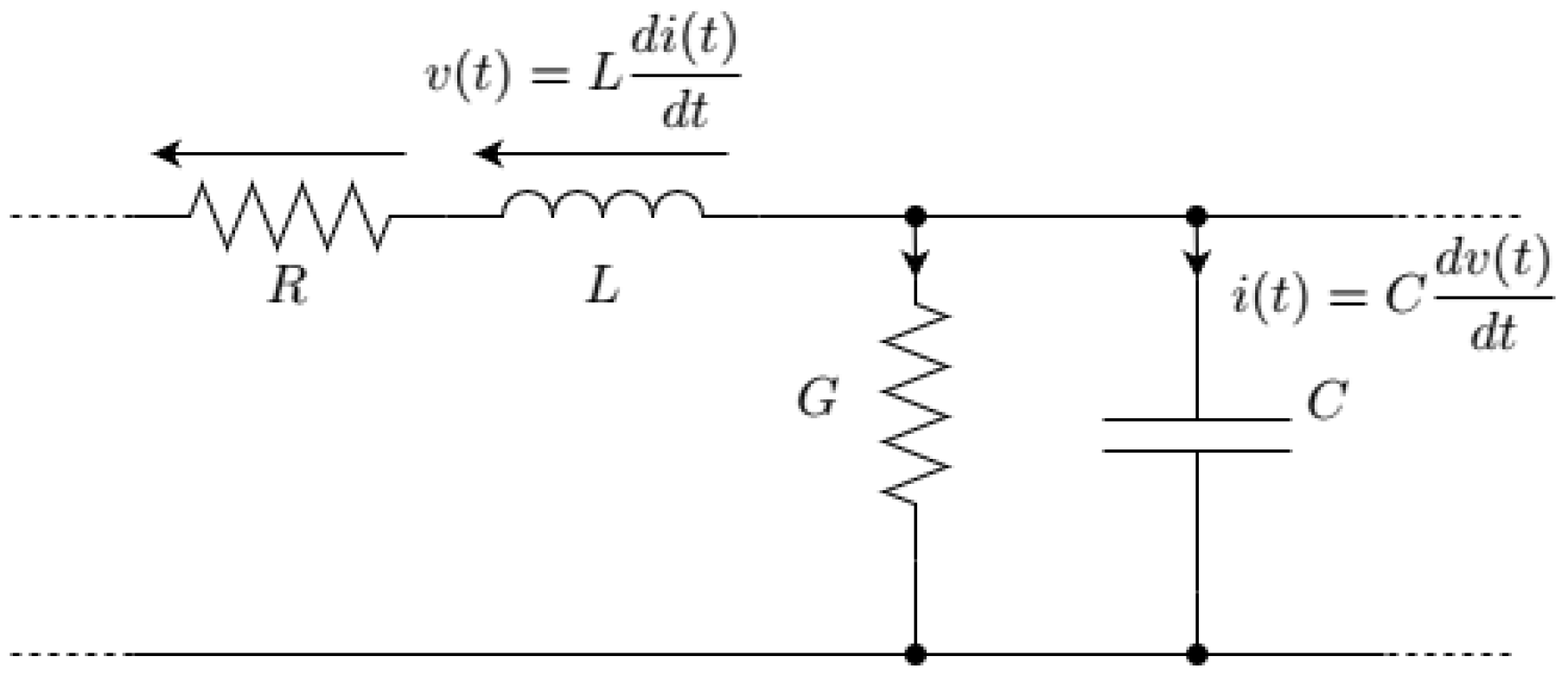
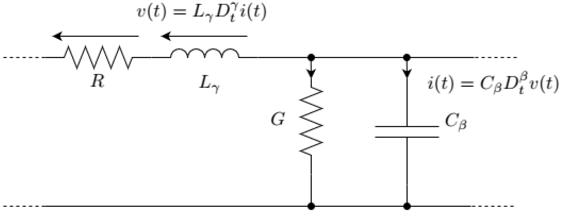
2. FO Transmission Lines

The IO model is able to describe characteristics of the transmission line in a limited frequency range. It stems from the fact that, for THz frequencies, a conductor exhibits both frequency and spatial dispersion [9,10]. Hence, the loss term in the traditional RLGC model with IO elements (see Figure 1) becomes insufficient if we want to describe the dispersion and non-quasi-static effects. It may further result in causality problems in the time-domain analysis. However, the FO RLGC model of the transmission line (see Figure 2) [9,10,22,23] can describe these effects in the THz frequency range.
In [9,10], a causal and compact FO transmission-line model for THz frequencies is developed for CMOS on-chip conductor. Due to the inclusion of frequency-dependent losses and non-quasi-static effects, a good agreement of characteristic impedance is observed between the FO model and the measurements up to 110 GHz. On the other hand, the traditional IO RLGC model provides an agreement between the model and the measurements only up to 10 GHz. These results clearly demonstrate the advantages of the FO transmission-line modeling. In Refs. [9,10], an FO derivative is applied, which guarantees the appropriate behavior in the frequency domain. That is, the authors apply the Riemann–Liouville definition with a base point at , but its Fourier-domain properties actually imply that the Grünwald–Letnikov definition is applied. However, as shown below, the circuit-level modeling of FO transmission lines may be problematic, due to the multitude of definitions of FO derivative operators. Hence, not every FO derivative may be applied, in a reasonable way, to the circuit-level modeling.
Let us consider the transmission line in Figure 2. Then, the voltage v = v ( x , t ) and the current i = i ( x , t ) along the line in the x direction are solutions to the following set of equations:
v x = R i L γ D t γ i
i x = G v C β D t β v
where γ , β ( 0 , 1 ] are fixed parameters. Differentiating both equations with respect to x and substituting (1) in (2) and vice versa (with the use of D x D t α = D t α D x property), the FO telegraph equations [23] are obtained as follows:
2 v x 2 = R G v + R C β D t β v + L γ G D t γ v + L γ C β D t γ D t β v
2 i x 2 = R G i + R C β D t β i + L γ G D t γ i + L γ C β D t β D t γ i .
Let us consider the phasor representation of the voltage and the current along the line
v = ( V e j ω t )
i = ( I e j ω t )
where V = V ( x ) and I = I ( x ) are, respectively, voltage and current phasors which are functions of the spatial variable x only and ω denotes the angular frequency. From (1) and the phasor representation (5) and (6), one obtains
V ( x ) x e j ω t + R I ( x ) e j ω t = L γ I ( x ) D t γ e j ω t
and
V ( x ) x + R I ( x ) = e j ω t L γ I ( x ) D t γ e j ω t .
For the left-hand side of (8), not depending on t, in order to apply the phasor representation to (1) and (2), one has to assume that the fractional-derivative operator D t α satisfies a certain property assuring that the right-hand side of the above equation does not depend on t either. This issue is addressed in the next section.

3. FO Derivative Properties Necessary for Applications in Circuit Theory

Several attempts have already been made to specify the conditions constituting the FO derivative [15,16,24]. Furthermore, these conditions have also been discussed with regard to possible applications in electromagnetism [17,25]. In this section, we would like to formulate a set of properties which would allow for applying the FO derivative concept in the circuit theory.
It is assumed that the considered functions are sufficiently regular (i.e., smooth enough) for the FO derivative operator D α ( α > 0 ) to be applied. Moreover, we assume that the functions are smooth enough for the sequence of derivatives D x and D t α to be changed, i.e., D x D t α = D t α D x (in practice, we may require that v ( x , t ) and i ( x , t ) are functions of the class C 2 ). Let us consider the function f ( t ) defined in the entire real line for which the bilateral Laplace transformation can be defined
f ^ = L { f ( t ) } = + f ( t ) e s t d t .
It is identical to the unilateral Laplace transformation given by
f ^ = L { f ( t ) } = 0 + f ( t ) e s t d t
for causal functions (i.e., f ( t ) = 0 for t < 0 ).
In our opinion, FO derivatives employed in the circuit theory should satisfy the following properties:
  • Identity
    D 0 f ( t ) = f ( t ) .
  • Compatibility with IO derivative
    D α f ( t ) = d α d t α f ( t ) , α N .
  • Compatibility with IO integral
    D α f ( t ) = f ( t ) d α t , α N .
  • Linearity
    D α ( a f ( t ) + b g ( t ) ) = a D α f ( t ) + b D α g ( t ) .
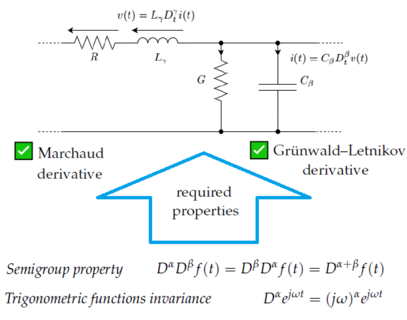
  • Semigroup property (also called the index law)
    D α D β f ( t ) = D β D α f ( t ) = D α + β f ( t ) , α , β R .
    This property is sometimes validated under additional assumptions, namely that, for example, either α , β < 0 or 0 < α , β , α + β < 1 . As it is noticed in [18], the condition (15) may not be satisfied for widely applied definitions of FO derivatives.
  • Trigonometric functions invariance
    D α e j ω t = ( j ω ) α e j ω t
    where j = 1 . The domain of the complex power function s s α is chosen so that it contains the complex right half-plane s > 0 . Hence,
    ( j ω ) α = | ω | α e j α sgn ( ω ) π 2 .
    It may be concluded from (7) and (8) that the phasor analysis can generally be applied when
    D α e j ω t = c ( ω , α ) e j ω t
    where c ( ω , α ) is a certain constant depending on ω and α . However, the specific condition (16) seems to be a much more natural one to be postulated. One should note that it is required for the analysis of circuits with zero initial conditions for which the substitution s = j ω in the Laplace domain provides the solution in the phasor domain.
  • Constant function derivative
    D α c = 0
    where c = c o n s t and α > 0 . This property results from the trigonometric functions invariance because one obtains (19) from (16) when ω = 0 .
As it has been mentioned at the end of the previous section, the phasor representation of the transmission-line Equations (1) and (2) leads to the Formula (8) and the conclusion that (18) must be satisfied. Assuming the condition (16), one obtains from (1) and (2) the following equations describing the FO transmission line in the frequency domain:
V x = [ R + ( j ω ) γ L γ ] I
I x = [ G + ( j ω ) β C β ] V .
Substituting (20) in (21) and vice versa, telegraph equations are obtained in the frequency domain as follows:
2 V 2 x = [ R + ( j ω ) γ L γ ] [ G + ( j ω ) β C β ] V
2 I 2 x = [ R + ( j ω ) γ L γ ] [ G + ( j ω ) β C β ] I .
It shows that the voltage and current phasors satisfy the same equation in the frequency domain. Hence, the time-domain functions representing the voltage or the current are taken from the same linear space of inverse Fourier transforms of solutions to (22) or (23), respectively.
A simple but important calculation shows that the fractional derivative satisfying the linearity (14) and the trigonometric functions invariance property (16) commutes on the linear space spanned by all trigonometric functions
sin ω t = e j ω t e j ω t 2 j
cos ω t = e j ω t + e j ω t 2 .
Moreover, the condition (16) implies that, for all linear combinations of trigonometric functions, not only D t α and D t β commute, but also the semigroup property (15) holds true. Naturally, one cannot conclude from this that the FO derivatives D t α and D t β commute in their entire domain. However, if one may identify such a function space C where the derivatives D t α are continuous in C , and the space of all trigonometric functions is dense in C , then surely
D t α D t β f = D t β D t α f = D t α + β f , for f C .
As shown, the voltage and current phasors satisfy the same Equations (22) and (23) in the frequency domain. On the other hand, the situation is different in the time domain, see (3) and (4). One can notice that the voltage and the current satisfy the same telegraph equation if and only if β = γ or the FO operators commute (i.e., D t γ D t β = D t β D t γ ). For β = γ = 1 , and assuming the property (12), one obtains the telegraph equation [26] for the traditional RLGC model of the transmission line with IO elements. However, having different equations for the voltage and the current, one may expect that their solution spaces can also be different, which would contradict the phasor domain observations. Hence, the symmetry of equations for the voltage and the current is a strong argument supporting the requirement of the semigroup property (15). Quite recently, Atangana and Gómez-Aguilar discussed the role of the definitions which do not satisfy the semigroup property [27,28], but their arguments do not seem to be applicable in the discussed context.
Hence, for the definitions of FO derivatives, which do not satisfy (16), one cannot apply the phasor analysis to the transmission lines. On the other hand, for the definitions of FO derivatives, which satisfy both (15) and (16), we may be sure that the time-domain FO telegraph Equations (3) and (4) are consistent with the frequency-domain formulation (22) and (23). In the next section, we review popular definitions of fractional derivatives from this perspective.

4. FO Derivatives

Let us assume that the considered function f : R R is defined on the real line. The presented definitions of FO derivatives have left- and right-sided versions. In our investigations, only the left-sided version is considered. These approaches are symmetrical and the left-sided version operates on past times; hence, it is closer to the concept of causality. It is worth noticing that both Riemann–Liouville and Caputo derivatives are defined with the use of a base point. The classical approach assumes that the base point a R is a finite number, but the definitions may also be extended to a = . Usually, due to the causality assumption, a = 0 is selected, and the domain of the function f can be restricted to the interval [ 0 , + ) .
There are numerous literature sources presenting applications of FO models in the circuit modeling and simulations. They refer to different definitions of FO derivatives; sometimes, a single paper refers to several FO models, built by means of various definitions. In the list below, we try to collect the papers referring to different definitions of fractional derivatives applied in the circuit theory. We must be very careful though because it sometimes happens that the same mathematical concept appears under different names, or the same name refers to different concepts. The list presented below refers to the definitions considered in this paper, with the names of derivatives not necessarily compatible with those given in the original source. For instance, we are not able to find the name of the Liouville derivative in the papers referring to the circuit theory, but there are several references to the Riemann–Liouville derivative with the base point a = (which refers to the same concept). The Caputo derivative sometimes appears as the Liouville–Caputo derivative, while the Liouville–Caputo derivative is sometimes called the Caputo derivative with the base point a = . The Caputo–Fabrizio may appear as Caputo–Fabrizio–Caputo derivative, while Atangana–Baleanu derivative may also be called Atangana–Baleanu–Caputo derivative.
References to various definitions of FO derivatives applied in the circuit theory are listed below:

4.1. Riemann–Liouville

The Riemann–Liouville integral is defined as
J α f ( t ) = 1 Γ ( α ) a t f ( τ ) ( t τ ) α 1 d τ
where α > 0 is the order of integration, Γ is the Gamma function, and a is the fixed base point. Hence, the Riemann–Liouville derivative of the order α ( n 1 , n ) is defined as
D α f ( t ) = D n J n α f ( t ) .
The Riemann–Liouville derivative does not satisfy neither (15) nor (16) in general. That is, the semigroup property is valid in a limited sense only, i.e., for α , β , α + β ( 0 , 1 ) . The semigroup property for the Riemann–Liouville integral is discussed in [24] [Section 3.2]. Some counterexamples (actually related to fractional differential equations) are presented in [77] (see Example 6.2 and Remark 5). For instance, the base point a = 0 leads to the derivatives of the sine and cosine functions which are non-elementary functions (refer to e.g., [78] [Propositions 11, 12] )
D α sin ( ω t ) = t α 2 E 1 , 1 α ( j ω t ) + E 1 , 1 α ( j ω t )
D α cos ( ω t ) = t α 2 E 1 , 1 α ( j ω t ) E 1 , 1 α ( j ω t )
where E α , β ( z ) is the generalized Mittag–Leffler function.
The Laplace transform of the FO derivative of the order α ( α [ n 1 , n ) where n N ) for the function f : [ 0 , + ) R can be calculated as [6] [Formula (1.85)]
L { D α f ( t ) } = s α L { f ( t ) } k = 0 n 1 s k [ D α k 1 f ( t ) ] t = 0 .

4.2. Caputo

The Caputo derivative is defined similarly to the Riemann–Liouville derivative (28), but with the reversed order of the FO integration and the IO derivative operators
D α f ( t ) = J n α D n f ( t )
where α ( n 1 , n ) . It is also possible to define it based on the Riemann–Liouville integral (see [6] [Formula (1.12)] or [5] [Formula (2.4.1)]) as
C D α f ( t ) = R L D α f ( t ) k = 0 n 1 t k k ! f ( k ) ( 0 )
where C D α is the Caputo derivative and R L D α is the Riemann–Liouville derivative with the same base point a = 0 . Both definitions (32) and (33) are equivalent for a function f of the class C n , although the definition (33) formally requires only the existence of ( n 1 )-th derivative in the neighborhood of the base point a = 0 . The Formula (33) applied to the function f ( t ) = sin t for α ( 0 , 1 ) shows that (29) is also valid for the Caputo derivative with the base point a = 0 . Therefore, the Caputo derivative does not satisfy (16)—for exact formulas, see [78] (Propositions 11 and 12). Moreover, the semigroup property (15) is not generally valid for this definition, refer to [77]—particularly to Example 6.1 therein.
The Laplace transform of the FO Caputo derivative of the order α ( n 1 , n ] (where n N ) of the function f : [ 0 , + ) R can be calculated as [6] [Formula (1.88)]
L { D α f ( t ) } = s α L { f ( t ) } k = 0 n 1 s α k 1 f ( k ) ( 0 ) .

4.3. Liouville–Caputo

The Liouville–Caputo derivative is defined as the Caputo derivative with the base point a = (see Formula (49) in [79])
D α f ( t ) = J n α D n f ( t ) = 1 Γ ( n α ) t ( t τ ) n α 1 D n f ( τ ) d τ
where α > 0 is the order of integration, α ( n 1 , n ) for a certain n N .
The trigonometric functions invariance property (16) holds true, which can be directly verified by the Formula (5) in Table 9.2 in [4]. The formulas
J β ( sin ω t ) = ω β sin ( ω t β π 2 )
J β ( cos ω t ) = ω β cos ( ω t β π 2 )
are satisfied for ω > 0 and β ( 0 , 1 ) . Before we continue, let us note that, for n N , one obtains
D n sin ( ω t + ϕ ) = ω n sin ( ω t + ϕ + n π 2 )
D n cos ( ω t + ϕ ) = ω n cos ( ω t + ϕ + n π 2 ) .
For α > 0 and ω > 0 , one obtains
D α ( cos ω t + j sin ω t ) = J n α D n ( cos ω t + j sin ω t ) =
ω n J n α ( cos ( ω t + n π 2 ) + j sin ( ω t + n π 2 ) ) =
ω α ( cos ( ω t α π 2 ) + j sin ( ω t α π 2 ) ) = ( j ω ) α e j ω t .
Similar derivations can be obtained for ω < 0 . One should note that, in the case of the Liouville–Caputo derivative, the trigonometric functions invariance property (16) holds true for ω = 0 as well.
In general, the semigroup property (15) does not hold true for the Liouville–Caputo derivative. Let us note that, for the function f : R R , where f ( t ) = 0 for t 0 , the Liouville–Caputo derivative coincides with the Caputo derivative (defined in Section 4.2), with the base point a = 0 . This is why, for any example mentioned in Section 4.2, and where
D 0 α D 0 β f ( t ) D 0 α + β f ( t ) ,
one obtains
D α D β f ( t ) D α + β f ( t ) .
In (41), D 0 α denotes the Caputo derivative with the base point a = 0 . Thus, in general, the semigroup property (15) does not hold true for the Liouville–Caputo derivative.

4.4. Liouville

In the literature (see [4], [Formulas (5.6) and (5.7)] and also [15,78]) the Riemann–Liouville derivative with the base point a = is referred to as the Liouville derivative. Let us consider this definition
D α f ( t ) = D n 1 Γ ( n α ) t f ( τ ) ( t τ ) n α 1 d τ
where α > 0 is the order of integration and α ( n 1 , n ) for a certain n N . The definition requires that the integral on the right side of (43) exists. One may assume that the function f vanishes at quickly enough (e.g., for α ( 0 , 1 ) , f L p ( R 1 ) , where 1 p < 1 / ( n α ) —refer to the discussion at the beginning of Chapter 2 in [4]), which guarantees that the integral exists in the Lebesgue sense. One may also focus on periodic functions (with an integral equal to 0 over the period)—then, the integral exists in the sense of Riemann for any α > 0 (and the integral is conditionally convergent). The case of periodic functions corresponds to the concept of the so-called Weyl derivative (see, e.g., [4] (Section 19)).
It occurs that, for α ( 0 , 1 ) and the functions which are good enough (e.g., continuously differentiable and vanishing at quickly enough), this definition is equivalent to the definition of the Marchaud derivative (for an exact definition see Section 4.5 below). At the same time, the Marchaud derivative is much more general as it allows for a larger domain not requiring that the function vanishes at (including the constant function). This topic is covered in detail in Section 5.4. of [4].
The trigonometric functions invariance property (16) can be checked in a similar way as in Section 4.3 above, i.e., Equations (36) and (37) with β = n α should be n-times differentiated to obtain the fractional Liouville derivative of the order α
D α ( cos ω t + j sin ω t ) =
D n ω α n ( cos ( ω t ( n α ) π 2 ) + j sin ( ω t ( n α ) π 2 ) =
ω α ( cos ( ω t α π 2 ) + j sin ( ω t α π 2 ) =
ω α e j ω t e j α π 2 = ( j ω ) α e j ω t
for any α > 0 . The case of ω < 0 may be considered in a similar way. One should also note that, for ω = 0 (corresponding to the constant function), the trigonometric functions invariance property (16) does not hold true because the integral t ( t τ ) n α 1 d τ does not exist.
Let us notice that, for the function f : R R , where f ( t ) = 0 for t 0 , the Liouville derivative coincides with the Riemann–Liouville derivative (defined in Section 4.1) with the base point a = 0 . This is why, for any example mentioned in Section 4.1, and where
D 0 α D 0 β f ( t ) D 0 α + β f ( t ) ,
one obtains
D α D β f ( t ) D α + β f ( t ) .
Here, D 0 α denotes the Riemann–Liouville derivative with the base point a = 0 . Thus, the semigroup property (15) does not, in general, hold true for the Liouville derivative.

4.5. Marchaud

For the order of differentiation α ( 0 , 1 ) , the Marchaud derivative is given by
D α f ( t ) = α Γ ( 1 α ) 0 + f ( t ) f ( t τ ) τ 1 + α d τ .
This definition is equivalent (for α ( 0 , 1 ) ) to the Liouville derivative for a broad class of functions, i.e., for a class of sufficiently regular functions with an appropriate behaviour at , as discussed in [4] (Section 5.4). There are also very important differences between both definitions. The first one is that the Marchaud derivative can be calculated for a broader class of functions than the Liouville derivative, including constant functions. The other is that the natural extension of the Marchaud definition differs from the Liouville definition for α > 1 . The extension of the Marchaud definition for α > 1 can be formulated in two directions (refer to [4] (Section 5.5), [6] (Section 1.3.1), and [80] for a historical perspective). First of all, when α ( n 1 , n ) and n N , then
D α f ( t ) = D α ( n 1 ) D n 1 f ( t ) = { α } Γ ( 1 { α } ) 0 + f ( n 1 ) ( t ) f ( n 1 ) ( t τ ) τ 1 + { α } d τ
where { α } = α ( n 1 ) , and f is assumed to be sufficiently smooth, e.g., f C n 1 ( R ) with f ( n 1 ) bounded. Another approach is to replace the first-order difference in the numerator in (47) with the n-th order difference Δ τ n f ( t )
D α f ( t ) = c 0 + Δ τ n f ( t ) τ 1 + α d τ
with an appropriate constant c > 0 . This attitude does not require any differentiability assumptions on f. Moreover, the definition of the Marchaud derivative (49) is naturally equivalent to the Grünwald–Letnikov definition discussed in Section 4.7 below (for a broad class of functions, covering periodic functions and L p ( R ) functions for p [ 1 , + ) —refer to Theorems 20.2 and 20.4 in [4]). Because of the equivalence, the discussion of properties of the Marchaud derivative is given in Section 4.7, devoted to the Grünwald–Letnikov derivative. We should also mention that the recent survey paper [81] discusses both approaches in detail.

4.6. Two-Sided Fractional Ortigueira–Machado Derivative

In the recently published papers [82,83], the concept of unified derivatives is introduced, which covers among others (as special cases) the Grünwald–Letnikov, Liouville and Liouville–Caputo concepts. The definition which employs two parameters, i.e., α (derivative order) and θ (asymmetry parameter), is introduced and formulated by means of an appropriate behaviour of the Fourier transform. Formula (28) in [83] (see also Definition 2 in [82]) defines the derivative D θ α f ( t ) of the function f : R R as
F ( D θ α f ) ( ω ) = | ω | α e j π 2 θ sgn ( ω ) F ( f ) ( ω ) .
Due to the multitude of attitudes to the Fourier transformation definition, we must be very precise. The definition we use follows the one given in [83]
F ( f ) ( ω ) = + f ( t ) e j ω t d t
and
F 1 ( F ) ( t ) = 1 2 π + F ( ω ) e j ω t d t .
In view of the definition (50), the semigroup property (15) is naturally satisfied (see Property 3 following Definition 3.1 in [83]), but it must be understood in an appropriate way as
D θ α D η β f ( t ) = D θ + η α + β f ( t ) .
Formally, the derivative depends on two independent parameters α and θ . However, when one considers the definition from the perspective of the FO model of the transmission line (1) and (2), it is difficult to find physical interpretation of the asymmetry parameter θ . Hence, it is reasonable to assume that the asymmetry parameter θ depends on the order of the derivative, i.e., θ = θ ( α ) . Then, the Formula (53) implies that
D θ ( β ) β D θ ( α ) α f ( t ) = D θ ( β ) + θ ( α ) β + α f ( t ) .
On the other hand, the semigroup property (15) requires that
D θ ( β ) β D θ ( α ) α f ( t ) = D θ ( β + α ) β + α f ( t )
and, consequently, one has to assume that θ ( α + β ) = θ ( α ) + θ ( β ) . Hence, it is reasonable to assume that θ ( β ) is the linear map θ : R R and
θ ( α ) = Θ · α
for a fixed Θ R . From now on, we are going to use the following–and hopefully not confusing–notation
D Θ α f ( t ) = D Θ α α f ( t )
for θ ( α ) given by (56).
Let us now consider the trigonometric functions invariance property (16). As it can be seen, one obtains, by way of easy calculations (see also Property 1 following Definition 3.1 and Formula (29) in [83])
D Θ α e j ω t = | ω | α e j π 2 Θ α sgn ( ω ) e j ω t = e j π 2 ( Θ 1 ) α sgn ( ω ) ( j ω ) α e j ω t .
Thus, the trigonometric functions invariance property (16) is valid only when Θ = 1 . On the other hand, one may notice that the more general condition (18) holds true for any Θ with c ( ω , α ) = e j π 2 ( Θ 1 ) α sgn ( ω ) ( j ω ) α .

4.7. Grünwald–Letnikov

The Grünwald–Letnikov derivative of the order α > 0 is given by the discrete formula (refer to [4] (Formula (20.7)))
D α f ( x ) = lim h 0 + 1 h α m = 0 ( 1 ) m α m f ( x m h )
where α m = α ( α 1 ) . . . ( α m + 1 ) m ! . This definition satisfies both (15) (refer to [84] (Section 2.6.1)) and (16) (refer to [84] (Formula (2.65))). One should notice that the Grünwald–Letnikov derivative is a special case (for Θ = 1 , i.e., θ ( α ) = α ) of the Ortigueira–Machado derivative (see row 1 in Table 1 in [82]).
The bilateral Laplace transform of the derivative of the order α ( n 1 , n ) (where n N ) of the function f : R R can be calculated as [84] (Sections 2.7.3 and 2.8)
L { D α f ( t ) } = s α L { f ( t ) } , s > 0 .
As it has been mentioned, the Grünwald–Letnikov definition is equivalent to the Marchaud definition for a broad class of functions. To be more specific, the Marchaud definition in the sense of (49) is equivalent to the Grünwald–Letnikov derivative. Therefore, it satisfies both (15) and (16). Then, it easily leads to the observation that the definition (48) (which is given by the semigroup formula D α f ( t ) = D α ( n 1 ) D n 1 f ( t ) ) is equivalent to the definition (49) (naturally, for sufficiently smooth functions). Hence, one may conclude that the Marchaud definition, in any of the two versions given above, satisfies both (15) and (16).

5. Nonclassical Derivatives

There are not many references in the literature to ideas of FO derivatives applied in the FO circuit theory other than those listed above. Still, quite recently, some papers have appeared which refer to certain derivatives from the class of derivatives with nonsingular kernels (Caputo–Fabrizio, Atangana–Baleanu and Atangana–Koca–Caputo) and to a certain local fractional derivative (the so-called conformable derivative).
The definitions of these derivatives are presented below; for details and further references, we refer to [58] (where the first two derivatives appear under slightly different names, i.e., as Caputo–Fabrizio–Caputo and Atangana–Baleanu–Caputo, respectively) and the references therein. We further assume that α > 0 and α ( n 1 , n ) for a certain n N in the following definitions:
  • Caputo–Fabrizio (with the base point set at 0)
    D α f ( t ) = M ( α ) n α 0 t e α ( t τ ) n α D n f ( τ ) d τ
    where M ( α ) is a certain normalizing factor.
  • Atangana–Baleanu (with the base point set at 0)
    D α f ( t ) = B ( α ) n α 0 t E α ( α ( t τ ) α n α ) D n f ( τ ) d τ
    where E α denotes the (one-parameter) Mittag–Leffler function and B ( α ) is a certain normalizing factor.
  • Atangana–Koca–Caputo for α ( 0 , 1 ) (with the base point set at 0)
    D α f ( t ) = 1 g ( α ) 0 t E α , α α ( g ( α ) ( t τ ) α ) D f ( τ ) d τ
    where E α , α denotes the two-parameter Mittag–Leffler function and g ( α ) is a certain normalizing factor.
  • Conformable derivative
    D α f ( t ) = lim ϵ 0 f ( t + ϵ t 1 α ) f ( t ) ϵ .
These definitions appear to be very attractive due to certain advantages over classical definitions of FO derivatives. That is, the nonsingular kernel suggests access to faster and more accurate numerical methods (numerical methods usually lose their accuracy in the case of singularities), while the local definitions may be used to build models without memory effects (also making numerical solutions much easier to implement, as they do not require many resources to allow for looking into the past). It should be noted, though, that recently several papers have questioned whether such operators should be considered as belonging to the family of FO derivatives. For instance, Tarasov introduces, in [85], the principle of nonlocality for fractional derivatives. The principle states that, if a certain FO differential equation may be expressed by means of some other differential equation of IO, then the fractional derivative may not be considered nonlocal, hence (as the author says), it “cannot be used to describe processes and systems with non-locality and memory”. Then, it is shown that the local definition of a conformable derivative does not satisfy the principle of nonlocality. However, the more surprising fact may be observed for the Caputo–Fabrizio definition of the order α ( 0 , 1 ) defined by a certain integral, which also fails to satisfy the nonlocality principle. It is shown that a certain linear differential equation with the Caputo–Fabrizio derivative is actually equivalent to an appropriate first-order differential equation. The above-mentioned equivalence is valid only for functions which are regular enough, but it seems to be a good reason to consider such derivatives as nothing more than IO differential operators. The other arguments connected with this discussion may be found in [86,87,88]. The objection raised against the above-mentioned definitions is that they are defined as integral operators with nonsingular kernels (as the author states in [89]: “Fractional-order derivatives defined by continuous kernels are too restrictive”). In the case of all derivatives with nonsingular kernels (covering the definitions of Caputo–Fabrizio, Atangana–Baleanu and Atangana–Koca–Caputo), it is observed that their usage in some natural initial-value problems leads only to trivial solutions [89,90]. On the other hand, an alternative form of initial conditions is suggested in [91], in order to overcome these difficulties.
Nevertheless, as it is mentioned in [16], none of the derivatives of Caputo–Fabrizio and Atangana–Baleanu satisfy the semigroup property (15) in full generality, and nor does the conformable definition.

6. Conclusions

In this paper, the properties of FO derivatives required for the circuit-level modeling are considered. Potential problems related to generalization of the transmission-line equations with the use of FO derivatives are discussed. In FO models of transmission lines, the FO inductance can be useful for modeling of the skin effect, whilst the FO capacitance is able to model various non-idealities of dielectric media characteristics (e.g., accumulation of electric charge along the line and memory effects in dielectric polarization). In general, the time- and frequency-domain methods of the transmission-line analysis should return equivalent results. It is demonstrated that, in order to obtain the equivalence between the results in the time and frequency domains, the FO derivative modeling electrical characteristics of circuit elements should satisfy the semigroup condition and be representable in the phasor domain. From this point of view, we consider the following definitions of FO derivatives applied for the circuit-level modeling: Riemann–Liouville, Caputo, Liouville–Caputo, Liouville, Marchaud, Grünwald–Letnikov, Caputo–Fabrizio, Atangana–Baleanu, Atangana–Koca–Caputo and the conformable derivative. Out of the most popular approaches considered in this paper, only the Grünwald–Letnikov and Marchaud definitions (which are actually equivalent) satisfy the semigroup property and are naturally representable in the phasor domain. The generalization of this concept, i.e., the two-sided fractional Ortigueira–Machado derivative, satisfies the semigroup property, but its phasor representation is less natural. Other ideas (including the Riemann–Liouville and Caputo derivatives–with a finite or an infinite base point) seem to have limited applicability.

Author Contributions

Investigation, J.G., T.P.S. and D.T.; Supervision, T.P.S.; Writing—original draft, J.G., T.P.S. and D.T.; Writing—review and editing, J.G., T.P.S. and D.T. All authors have read and agreed to the published version of the manuscript.

Funding

This research received no external funding.

Conflicts of Interest

The authors declare no conflict of interest.

References

  1. Ortigueira, M.D. An introduction to the fractional continuous-time linear systems: The 21st century systems. IEEE Circuits Syst. Mag. 2008, 8, 19–26. [Google Scholar] [CrossRef] [Green Version]
  2. Elwakil, A.S. Fractional-order circuits and systems: An emerging interdisciplinary research area. IEEE Circuits Syst. Mag. 2010, 10, 40–50. [Google Scholar] [CrossRef]
  3. Freeborn, T.J. A Survey of Fractional-Order Circuit Models for Biology and Biomedicine. IEEE J. Emerg. Sel. Top. Circuits Syst. 2013, 3, 416–424. [Google Scholar] [CrossRef]
  4. Samko, S.G.; Kilbas, A.A.; Marichev, O.I. Fractional Integrals and Derivatives: Theory and Applications; Gordon and Breach: New York, NY, USA, 1993. [Google Scholar]
  5. Kilbas, A.A.; Srivastava, H.M.; Trujillo, J.J. Theory and Applications of Fractional Differential Equations; Elsevier Science: Amsterdam, The Netherlands, 2006. [Google Scholar]
  6. Li, C.; Zeng, F. Numerical Methods for Fractional Calculus; Chapman and Hall/CRC: Boca Raton, FL, USA, 2015. [Google Scholar]
  7. Al-daloo, M.; Soltan, A.; Yakovlev, A. Overview study of on-chip interconnect modeling approaches and its trend. In Proceedings of the 2018 7th International Conference on Modern Circuits and Systems Technologies (MOCAST), Thessaloniki, Greece, 7–9 May 2018; pp. 1–5. [Google Scholar]
  8. Al-Daloo, M.; Soltan, A.; Yakovlev, A. Advance Interconnect Circuit Modeling Design Using Fractional-Order Elements. IEEE Trans. Comput. Aided Des. Integr. Circuits Syst. 2020, 39, 2722–2734. [Google Scholar] [CrossRef]
  9. Shang, Y.; Fei, W.; Yu, H. A fractional-order RLGC model for Terahertz transmission line. In Proceedings of the 2013 IEEE MTT-S International Microwave Symposium Digest (MTT), Seattle, WA, USA, 2–7 June 2013; pp. 1–3. [Google Scholar] [CrossRef]
  10. Shang, Y.; Yu, H.; Fei, W. Design and Analysis of CMOS-Based Terahertz Integrated Circuits by Causal Fractional-Order RLGC Transmission Line Model. IEEE J. Emerg. Sel. Top. Circuits Syst. 2013, 3, 355–366. [Google Scholar] [CrossRef]
  11. Aydin, O.; Samanci, B.; Ozoguz, I.S. Characterization of Microstip Transmission Lines Using Fractional-order Circuit Model. Balk. J. Electr. Comput. Eng. 2018, 6, 266–270. [Google Scholar] [CrossRef]
  12. Chang, Y.-Y.; Yu, S.-H. A compact fractional-order model for Terahertz composite right/left handed transmission line. In Proceedings of the 2014 XXXIth URSI General Assembly and Scientific Symposium (URSI GASS), Beijing, China, 16–23 August 2014; pp. 1–4. [Google Scholar]
  13. Yang, C.; Yu, H.; Shang, Y.; Fei, W. Characterization of CMOS Metamaterial Transmission Line by Compact Fractional-Order Equivalent Circuit Model. IEEE Trans. Electron Devices 2015, 62, 3012–3018. [Google Scholar] [CrossRef]
  14. Shi, L.; Qiu, L.; Huang, X.; Zhang, F.; Wang, D.; Zhou, L.; Gao, J. Characterization of Si-BCB transmission line at millimeter-wave frequency by compact fractional-order equivalent circuit model. Int. J. Microw. Comput. Aided Eng. 2019, 29, e21685. [Google Scholar] [CrossRef]
  15. de Oliveira, E.C.; Machado, J.A.T. A review of definitions for fractional derivatives and integral. Math. Probl. Eng. 2014, 2014. [Google Scholar] [CrossRef] [Green Version]
  16. Teodoro, G.S.; Machado, J.T.; de Oliveira, E.C. A review of definitions of fractional derivatives and other operators. J. Comput. Phys. 2019, 388, 195–208. [Google Scholar] [CrossRef]
  17. Sikora, R.; Pawłowski, S. Fractional derivatives and the laws of electrical engineering. COMPEL Int. J. Comput. Math. Electr. Electron. Eng. 2018, 37, 1384–1391. [Google Scholar] [CrossRef]
  18. Sikora, R.; Pawłowski, S. On certain aspects of application of fractional derivatives in the electromagnetism. Prz. Elektrotechniczny 2018, 94, 101–104. [Google Scholar]
  19. Latawiec, K.J.; Stanisławski, R.; Łukaniszyn, M.; Czuczwara, W.; Rydel, M. Fractional-order modeling of electric circuits: Modern empiricism vs. classical science. In Proceedings of the 2017 Progress in Applied Electrical Engineering (PAEE), Koscielisko, Poland, 25–30 June 2017; pp. 1–4. [Google Scholar] [CrossRef]
  20. Jiang, Y.; Zhang, B. Comparative Study of Riemann–Liouville and Caputo Derivative Definitions in Time-Domain Analysis of Fractional-order Capacitor. IEEE Trans. Circuits Syst. II Express Briefs 2019, 67, 2184–2188. [Google Scholar] [CrossRef]
  21. Gulgowski, J.; Stefański, T.P.; Trofimowicz, D. On Applications of Fractional Derivatives in Circuit Theory. In Proceedings of the 2020 27th International Conference on Mixed Design of Integrated Circuits and System (MIXDES), Wroclaw, Poland, 25–27 June 2020; pp. 160–163. [Google Scholar]
  22. Gómez-Aguilar, J.F.; Dumitru, B. Fractional Transmission Line with Losses. Z. Naturforschung A 2014, 69, 539–546. [Google Scholar] [CrossRef] [Green Version]
  23. Cvetićanin, S.M.; Zorica, D.; Rapaić, M.R. Generalized time-fractional telegrapher’s equation in transmission line modeling. Nonlinear Dyn. 2017, 88, 1453–1472. [Google Scholar] [CrossRef]
  24. Ortigueira, M.D.; Tenreiro Machado, J. What is a Fractional Derivative? J. Comput. Phys. 2015, 293, 4–13. [Google Scholar] [CrossRef]
  25. Gulgowski, J.; Stefanski, T.P. On Applications of Fractional Derivatives in Electromagnetic Theory. 2020; submitted for publication in conference proceedings. [Google Scholar]
  26. Weisstein, E.W. “Telegraph Equation”. From MathWorld—A Wolfram Web Resource. 2020. Available online: https://mathworld.wolfram.com/TelegraphEquation.html (accessed on 30 August 2020).
  27. Atangana, A.; Gómez-Aguilar, J.F. Decolonisation of fractional calculus rules: Breaking commutativity and associativity to capture more natural phenomena. Eur. Phys. J. Plus 2018, 133, 166. [Google Scholar] [CrossRef]
  28. Atangana, A.; Gómez-Aguilar, J. Fractional derivatives with no-index law property: Application to chaos and statistics. Chaos Solitons Fractals 2018, 114, 516–535. [Google Scholar] [CrossRef]
  29. Zahra, W.; Hikal, M.; Bahnasy, T.A. Solutions of fractional order electrical circuits via Laplace transform and nonstandard finite difference method. J. Egypt. Math. Soc. 2017, 25, 252–261. [Google Scholar] [CrossRef]
  30. Sene, N. Fractional input stability for electrical circuits described by the Riemann–Liouville and the Caputo fractional derivatives. AIMS Math. 2019, 4, 147–165. [Google Scholar] [CrossRef]
  31. Chen, L.; Wu, X.; Xu, L.; Lopes, A.M.; Tenreiro Machado, J.; Wu, R.; Ge, S. Analysis of a rectangular prism n-units RLC fractional-order circuit network. Alex. Eng. J. 2020. [Google Scholar] [CrossRef]
  32. Alsaedi, A.; Nieto, J.J.; Venktesh, V. Fractional electrical circuits. Adv. Mech. Eng. 2015, 7, 1687814015618127. [Google Scholar] [CrossRef]
  33. Gómez-Aguilar, J.; Yépez-Martínez, H.; Escobar-Jiménez, R.; Astorga-Zaragoza, C.; Reyes-Reyes, J. Analytical and numerical solutions of electrical circuits described by fractional derivatives. Appl. Math. Model. 2016, 40, 9079–9094. [Google Scholar] [CrossRef]
  34. Lopes, A.; Tenreiro Machado, J. Fractional-order model of a nonlinear inductor. Bull. Pol. Acad. Sci. Tech. Sci. 2019, 67, 61–67. [Google Scholar] [CrossRef]
  35. Stefanski, T.P.; Gulgowski, J. Electromagnetic-based derivation of fractional-order circuit theory. Commun. Nonlinear Sci. Numer. Simul. 2019, 79, 104897. [Google Scholar] [CrossRef]
  36. Moreles, M.A.; Lainez, R. Mathematical modeling of fractional order circuit elements and bioimpedance applications. Commun. Nonlinear Sci. Numer. Simul. 2017, 46, 81–88. [Google Scholar] [CrossRef]
  37. Kaczorek, T. Selected Problems of Fractional Systems Theory; Springer: Berlin/Heidelberg, Germany, 2011. [Google Scholar]
  38. Kaczorek, T. Positive fractional linear electrical circuits. In Photonics Applications in Astronomy, Communications, Industry, and High-Energy Physics Experiments 2013; Romaniuk, R.S., Ed.; International Society for Optics and Photonics, SPIE: Bellingham, WA, USA, 2013; Volume 8903, pp. 481–494. [Google Scholar] [CrossRef]
  39. Kaczorek, T.; Rogowski, K. Fractional Linear Systems and Electrical Circuits; Springer International Publishing: Cham, Switzerland, 2015. [Google Scholar]
  40. Gómez, F.; Rosales, J.; Guía, M. RLC electrical circuit of non-integer order. Cent. Eur. J. Phys. 2013, 11, 1361–1365. [Google Scholar] [CrossRef] [Green Version]
  41. Banchuin, R.; Chaisricharoen, R. The analysis of active circuit in fractional domain. In Proceedings of the 2018 International ECTI Northern Section Conference on Electrical, Electronics, Computer and Telecommunications Engineering (ECTI-NCON), Chiang Rai, Thailand, 25–28 February 2018; pp. 21–24. [Google Scholar]
  42. Rosales, J.; Filoteo, J.; Gonzalez, A. A comparative analysis of the RC circuit with local and non-local fractional derivatives. Rev. Mex. Fis. 2018, 64, 647–654. [Google Scholar] [CrossRef] [Green Version]
  43. Puşcaşu, S.V.; Bibic, S.M.; Rebenciuc, M.; Toma, A.; Nicolescu, D. Aspects of Fractional Calculus in RLC Circuits. In Proceedings of the 2018 International Symposium on Fundamentals of Electrical Engineering (ISFEE), Bucharest, Romania, 1–3 November 2018; pp. 1–5. [Google Scholar]
  44. Shah, P.V.; Patel, A.D.; Salehbhai, I.A.; Shukla, A.K. Analytic Solution for the Electric Circuit Model in Fractional Order. Abstr. Appl. Anal. 2014, 2014, 343814. [Google Scholar] [CrossRef]
  45. Sene, N.; Gómez-Aguilar, J. Analytical solutions of electrical circuits considering certain generalized fractional derivatives. Eur. Phys. J. Plus 2019, 134, 1–14. [Google Scholar] [CrossRef]
  46. Magesh, N.; Saravanan, A. Generalized Differential Transform Method for Solving RLC Electric Circuit of Non-Integer Order. Nonlinear Eng. 2018, 7, 127–135. [Google Scholar] [CrossRef] [Green Version]
  47. Sowa, M.; Majka, Ł. Ferromagnetic core coil hysteresis modeling using fractional derivatives. Nonlinear Dyn. 2020, 101, 775–793. [Google Scholar] [CrossRef]
  48. Guía, M.; Gómez, F.; Rosales, J. Analysis on the time and frequency domain for the RC electric circuit of fractional order. Cent. Eur. J. Phys. 2013, 11, 1366–1371. [Google Scholar] [CrossRef] [Green Version]
  49. Abro, K.A.; Atangana, A. Mathematical analysis of memristor through fractal-fractional differential operators: A numerical study. Math. Methods Appl. Sci. 2020, 43, 6378–6395. [Google Scholar] [CrossRef]
  50. Abro, K.; Memon, A.; Memon, A. Functionality of circuit via modern fractional differentiations. Analog. Integr. Circuits Signal Process. 2019, 99, 11–21. [Google Scholar] [CrossRef]
  51. R-Smith, N.A.; Brančík, L. Nonuniform lossy transmission lines with fractional-order elements using NILT method. In Proceedings of the 2017 Progress in Electromagnetics Research Symposium-Fall (PIERS-FALL), Singapore, 19–22 November 2017; pp. 2540–2547. [Google Scholar]
  52. Jakubowska-Ciszek, A.; Walczak, J. Analysis of the transient state in a parallel circuit of the class RLβCα. Appl. Math. Comput. 2018, 319, 287–300. [Google Scholar]
  53. Kaczorek, T. Minimum Energy Control of Fractional Positive Electrical Circuits with Bounded Inputs. Circuits Syst. Signal Process. 2016, 35, 1815–1829. [Google Scholar] [CrossRef] [Green Version]
  54. Kaczorek, T. Positive Linear Systems Consisting of n Subsystems With Different Fractional Orders. IEEE Trans. Circuits Syst. I Regul. Pap. 2011, 58, 1203–1210. [Google Scholar] [CrossRef]
  55. Kaczorek, T. An Extension of the Cayley-Hamilton Theorem to Different Orders Fractional Linear Systems and Its Application to Electrical Circuits. IEEE Trans. Circuits Syst. II Express Briefs 2019, 66, 1169–1171. [Google Scholar] [CrossRef]
  56. Kaczorek, T. Singular fractional linear systems and electrical circuits. Int. J. Appl. Math. Comput. Sci. 2011, 21, 379–384. [Google Scholar] [CrossRef]
  57. Hristov, J. Electrical Circuits of Non-integer Order: Introduction to an Emerging Interdisciplinary Area with Examples. In Analysis and Simulation of Electrical and Computer Systems; Mazur, D., Gołębiowski, M., Korkosz, M., Eds.; Springer International Publishing: Cham, Switzerland, 2018; pp. 251–273. [Google Scholar]
  58. Gomez-Aguilar, J.F. Fundamental solutions to electrical circuits of non-integer order via fractional derivatives with and without singular kernels. Eur. Phys. J. Plus 2018, 133. [Google Scholar] [CrossRef]
  59. Sene, N. Stability analysis of electrical RLC circuit described by the Caputo-Liouville generalized fractional derivative. Alex. Eng. J. 2020, 59, 2083–2090. [Google Scholar] [CrossRef]
  60. Gómez-Aguilar, J.; Escobar-Jiménez, R.; Olivares-Peregrino, V.; Taneco-Hernández, M.; Guerrero-Ramírez, G. Electrical circuits RC and RL involving fractional operators with bi-order. Adv. Mech. Eng. 2017, 9, 1687814017707132. [Google Scholar] [CrossRef]
  61. Morales-Delgado, V.; Gómez-Aguilar, J.; Taneco-Hernandez, M. Analytical solutions of electrical circuits described by fractional conformable derivatives in Liouville-Caputo sense. AEU Int. J. Electron. Commun. 2018, 85, 108–117. [Google Scholar] [CrossRef]
  62. Gómez-Aguilar, J.; Morales-Delgado, V.; Taneco-Hernández, M.; Baleanu, D.; Escobar-Jiménez, R.; Al Qurashi, M. Analytical Solutions of the Electrical RLC Circuit via Liouville-Caputo Operators with Local and Non-Local Kernels. Entropy 2016, 18, 402. [Google Scholar] [CrossRef]
  63. Tenreiro Machado, J.; Lopes, A.M. Fractional-order modeling of a diode. Commun. Nonlinear Sci. Numer. Simul. 2019, 70, 343–353. [Google Scholar] [CrossRef]
  64. Sowa, M. Harmonic Balance Methodology for Circuits with Fractional and Nonlinear Elements. Circuits Syst. Signal Process. 2018, 37, 4695–4727. [Google Scholar] [CrossRef] [Green Version]
  65. Stefański, T.P.; Gulgowski, J. Fractional Order Circuit Elements Derived from Electromagnetism. In Proceedings of the 2019 MIXDES—26th International Conference “Mixed Design of Integrated Circuits and Systems”, Rzeszów, Poland, 27–29 June 2019; pp. 310–315. [Google Scholar]
  66. Stefański, T.P.; Trofimowicz, D.; Gulgowski, J. Simulation of Signal Propagation Along Fractional-Order Transmission Lines. In Proceedings of the 2020 27th International Conference on Mixed Design of Integrated Circuits and System (MIXDES), Wroclaw, Poland, 25–27 June 2020; pp. 164–167. [Google Scholar]
  67. Martynyuk, V.; Ortigueira, M. Fractional model of an electrochemical capacitor. Signal Process. 2015, 107, 355–360. [Google Scholar] [CrossRef]
  68. Gómez-Aguilar, J.; Córdova-Fraga, T.; Escalante-Martínez, J.; Calderón-Ramón, C.; Escobar-Jiménez, R. Electrical circuits described by a fractional derivative with regular Kernel. Rev. Mex. Fís. 2016, 62, 144–154. [Google Scholar] [CrossRef] [Green Version]
  69. Abro, K.A.; Atangana, A. Numerical Study and Chaotic Analysis of Meminductor and Memcapacitor Through Fractal-Fractional Differential Operator. Arab. J. Sci. Eng. 2020. [Google Scholar] [CrossRef]
  70. Abro, K.A.; Memon, A.A.; Uqaili, M.A. A comparative mathematical analysis of RL and RC electrical circuits via Atangana-Baleanu and Caputo-Fabrizio fractional derivatives. Eur. Phys. J. Plus 2018, 133, 1–9. [Google Scholar] [CrossRef]
  71. Atangana, A.; Alkahtani, B.S.T. Extension of the resistance, inductance, capacitance electrical circuit to fractional derivative without singular kernel. Adv. Mech. Eng. 2015, 7, 1–6. [Google Scholar] [CrossRef]
  72. Atangana, A.; Nieto, J.J. Numerical solution for the model of RLC circuit via the fractional derivative without singular kernel. Adv. Mech. Eng. 2015, 7, 1–7. [Google Scholar] [CrossRef]
  73. Alizadeh, D.B.S.; Rezapour, S. Analyzing transient response of the parallel RCL circuit by using the Caputo-Fabrizio fractional derivative. Adv. Differ. Equ. 2020, 55, 1–19. [Google Scholar] [CrossRef]
  74. Sheikh, N.A.; Ching, D.L.C.; Ullah, S.; Khan, I. Mathematical and Statistical Analysis of Rl and RC Fractional-Order Circuits. Fractals 2020, 28, 1–7. [Google Scholar] [CrossRef]
  75. Gómez-Aguilar, J.F.; Atangana, A.; Morales-Delgado, V.F. Electrical circuits RC, LC, and RL described by Atangana-Baleanu fractional derivatives. Int. J. Circuit Theory Appl. 2017, 45, 1514–1533. [Google Scholar] [CrossRef]
  76. Martínez, L.; Rosales, J.; Carreño, C.; Lozano, J. Electrical circuits described by fractional conformable derivative. Int. J. Circuit Theory Appl. 2018, 46, 1091–1100. [Google Scholar] [CrossRef]
  77. Bhalekar, S.; Patil, M. Can we split fractional derivative while analyzing fractional differential equations? Commun. Nonlinear Sci. Numer. Simul. 2019, 76, 12–24. [Google Scholar] [CrossRef] [Green Version]
  78. Garrappa, R.; Kaslik, E.; Popolizio, M. Evaluation of Fractional Integrals and Derivatives of Elementary Functions: Overview and Tutorial. Mathematics 2019, 7, 407. [Google Scholar] [CrossRef] [Green Version]
  79. Shchedrin, G.; Smith, N.C.; Gladkina, A.; Carr, L.D. Exact results for a fractional derivative of elementary functions. SciPost Phys. 2017, 4, 29. [Google Scholar] [CrossRef] [Green Version]
  80. Ferrari, F. Weyl and Marchaud derivatives: A forgotten history. Mathematics 2018, 6, 6. [Google Scholar] [CrossRef] [Green Version]
  81. Rogosin, S.; Dubatovskaya, M. Letnikov vs. Marchaud: A survey on two prominent constructions of fractional derivatives. Mathematics 2018, 6, 3. [Google Scholar] [CrossRef] [Green Version]
  82. Ortigueira, M.D.; Machado, J.T. Fractional Derivatives: The Perspective of System Theory. Mathematics 2019, 7, 150. [Google Scholar] [CrossRef] [Green Version]
  83. Ortigueira, M.D. Two-sided and regularised Riesz-Feller derivatives. Math. Methods Appl. Sci. 2019. [Google Scholar] [CrossRef]
  84. Ortigueira, M.D. Fractional Calculus for Scientists and Engineers; Lecture Notes in Electrical Engineering; Springer: Berlin/Heidelberg, Germany, 2011. [Google Scholar]
  85. Tarasov, V.E. No nonlocality. No fractional derivative. Commun. Nonlinear Sci. Numer. Simul. 2018, 62, 157–163. [Google Scholar] [CrossRef] [Green Version]
  86. Tarasov, V.E. No violation of the Leibniz rule. No fractional derivative. Commun. Nonlinear Sci. Numer. Simul. 2013, 18, 2945–2948. [Google Scholar] [CrossRef] [Green Version]
  87. Ortigueira, M.D.; Tenreiro Machado, J. A critical analysis of the Caputo–Fabrizio operator. Commun. Nonlinear Sci. Numer. Simul. 2018, 59, 608–611. [Google Scholar] [CrossRef]
  88. Cresson, J.; Szafrańska, A. Comments on various extensions of the Riemann—Liouville fractional derivatives: About the Leibniz and chain rule properties. Commun. Nonlinear Sci. Numer. Simul. 2020, 82, 104903. [Google Scholar] [CrossRef] [Green Version]
  89. Stynes, M. Fractional-order derivatives defined by continuous kernels are too restrictive. Appl. Math. Lett. 2018, 85, 22–26. [Google Scholar] [CrossRef]
  90. Diethelm, K.; Garrappa, R.; Giusti, A.; Stynes, M. Why fractional derivatives with nonsingular kernels should not be used. Fract. Calc. Appl. Anal. 2020, 23, 610–634. [Google Scholar] [CrossRef]
  91. Sabatier, J. Fractional-Order Derivatives Defined by Continuous Kernels: Are They Really Too Restrictive? Fractal Fract. 2020, 4, 40. [Google Scholar] [CrossRef]
Figure 1. Unit cell of IO model of transmission line.
Energies 13 05768 g001
Figure 2. Unit cell of FO model of transmission line.
Energies 13 05768 g002
Publisher’s Note: MDPI stays neutral with regard to jurisdictional claims in published maps and institutional affiliations.

