Abstract
The interconnection of dynamic subsystems that share limited resources are found in many applications, and the control of such systems of subsystems has fueled significant attention from scientists and engineers. For the operation of such systems, model predictive control (MPC) has become a popular technique, arguably for its ability to deal with complex dynamics and system constraints. The MPC algorithms found in the literature are mostly centralized, with a single controller receiving the signals and performing the computations of output signals. However, the distributed structure of such interconnected subsystems is not necessarily explored by standard MPC. To this end, this work proposes hierarchical decomposition to split the computations between a master problem (centralized component) and a set of decoupled subproblems (distributed components) with activation constraints, which brings about organizational flexibility and distributed computation. Two general methods are considered for hierarchical control and optimization, namely Benders decomposition and outer approximation. Results are reported from a numerical analysis of the decompositions and a simulated application to energy management, in which a limited source of energy is distributed among batteries of electric vehicles.
1. Introduction
Several systems found in the industry and society emerge from the interconnection of dynamic subsystems that share limited resources [1,2]. Representative systems include stations for recharging electric vehicles, energy building management, and cooling fluid distribution in buildings, among others.
For instance, we can consider a building that has a Heating, Ventilation, and Air Conditioning (HVAC) as an example of a resource-constrained dynamic system. In this building, the cooling fluid is a limited resource shared among the rooms (subsystems), each with its energetic demand, depending on the number of users and the wall materials, among other factors. Another example appears in a water distribution system, which supplies the water demands of industries, houses, and commercial centers of a city. Thus, the water available in the water reservoir represents the limited resource at a specific time. Lastly, we can consider a charging station for electric vehicles (EVs), where each parked car generates an energy demand that can be supplied by the electric-power grid, photovoltaic panels, and even other batteries that are connected to the local grid. All of these systems presented depend on the distribution of limited resources (i.e., energy). Despite being interconnected systems, each subsystem (i.e., a vehicle with its battery being charged) does not need to know the state of another subsystem (i.e., the state-of-charge of another vehicle), only the amount of resources made available by the central system controller (master system) to the subsystem.
One of the control techniques typically applied to these interconnected systems is the Model Predictive Control (MPC), a control strategy widely used for energy applications, like microgrids [3,4] and photovoltaic applications [5]. In this context, there are two classes of strategies that can be approached for controlling such systems, the centralized control [6] and the decentralized control [7]. Although decentralized control is fast and scalable, the lack of coordination between distributed units can lead to poor performance or render the operation infeasible. Figure 1a illustrates the structure of this type of controller, where there is a controller for each system.
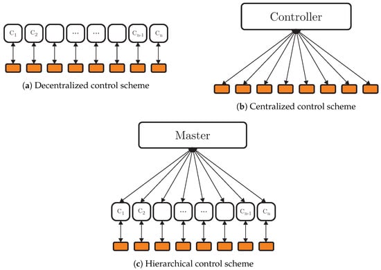
Figure 1.
Control schemes.
On the other hand, centralized control is capable of optimal performance, but the computational cost can become high, and the monolithic approach is less flexible. Figure 1b presents a scheme for centralized control, where there is just one controller that communicates with all systems.
As an alternative, some approaches combine the characteristics of decentralized and centralized controls, with emphasis on decomposition strategies that enable hierarchical control, which can be seen in Figure 1c, where there is a master problem that coordinates other controllers, so these controllers can be considered decoupled, having independent dynamics. Bilevel decomposition [8], Lagrangean decomposition [9], Benders decomposition [10], and Outer Approximation [11] are examples of such approaches.
In [12], the authors presented a hierarchical decomposition approach for MPC of dynamic systems using Bilevel, Lagrangean, and Benders decompositions. The authors reported results from a numerical analysis of the decompositions and a simulated application to the energy management of a building, in which a limited source of chilled water is distributed among HVAC units. The benefit of hierarchical decompositions is organizational, as they allow the control system to be reconfigured locally and expanded with reduced coordination. The signals communicated between the master and the subsystems are relatively simple, consisting of resource allocations (from the master to the subsystems), and cuts and derivatives/sensitivities (from the subsystems to the master). The master does not need to have detailed information about the subproblems in such a structure, making this approach ideal for distributed and intelligent systems.
Despite this potential of parallel computation, hierarchical and distributed algorithms are often slower than their centralized counterparts. Thus, the main benefit of a hierarchical decomposition is not computational but rather organizational as it facilitates the expansion and reconfiguration of the control system. This feature stems from the simple coordination scheme and reduced information communication [12]. In addition, it has already been shown in the literature that, by employing hierarchical decompositions, a reduction in computational time can be achieved by parallel computation, but not linearly as the number of cores increases [13].
Benders decomposition and Outer Approximation, such as Bilevel optimization, allow us to harness the structure of the problem, in the same manner, using parallel computing. Under specific and general conditions on the problems, Benders decomposition and Outer Approximation ensure convergence to the optimal solution [14]. These two decomposition strategies can be used to model activation variables, i.e., binary variables, to enable or disable the input of control signals into the system if necessary. In this sense, we extend the formulation previously presented in [12] (which only considered continuous variables) to include activation variables (binary)—which are able to individually define which subsystems are on or off—using Benders Decomposition and Outer Approximation.
The use of activation variables is particularly interesting when dealing with limited energy resources problems and can delegate to the hierarchical MPC the decisions regarding the activation/deactivation of units. The use of activation/deactivation variables can bring about additional flexibility for the controller to maximize the control objective. That is, instead of keeping several subsystems at low levels, choose to turn off specific subsystems to prioritize the energy supplied to others. It is worth remarking that the formulation with activation/deactivation constraints is more general than its counterpart with only continuous variables.
The usefulness of the proposed decompositions is illustrated in an application to the distributed charging of electric vehicles with the use of activation variables (i.e., the possibility to enable/disable certain charging stations).
Everything considered, the main contribution of this paper is a hierarchical formulation for management of energy systems sharing limited resources, while considering the possibility to activate/deactivate units (subsystems) by means of Benders Decomposition and Outer Approximation. These formulations, tailored for MPC applications, bring about organizational flexibility to the central control unit (master problem), which does not need detailed information of the subsystems; only signals regarding the allocated resources and solutions are communicated. Such a flexibility allows for plug-and-play technology, thus becoming compatible with intelligent and distributed systems.
The remainder of this paper is organized as follows: Section 2 presents the fundamental concepts for the development of the present research. Section 3 presents the proposed decompositions for MPC of resource-constrained dynamic systems with activation constraints. Numeral experiments regarding the decompositions, and an application to battery charging stations, with activation constraints are presented in Section 4. In conclusion, Section 5 gives the final remarks.
2. Background
2.1. Model Predictive Control
Model Predictive Control (MPC) has developed considerably over the last two decades; it is one of the few advanced control techniques that have significantly impacted industrial process control. This impact can be attributed to the fact that MPC is, perhaps, the most general way of posing the process control problem in the time domain, and the possibility to be applied in SISO (Single Input Single Output) and MIMO (Multiple Inputs Multiple Outputs) systems. Soft and hard constraints can be included in the formulation of the control law, through the solution of optimization problems, whereby an objective function is minimized over a prediction horizon [15].
In the literature, two of the most cited MPC strategies are the Dynamic Matrix Control (DMC) [16] and Generalized Predictive Control (GPC) [17,18]. Linear models are often used; in DMC, a step response model is used and, in GPC, a transfer function model. DMC is widely used in the industry due to the ease of obtaining this type of model, but it cannot be used with unstable systems [6]. State-space models have been increasingly used in the development of predictive controllers because they allow for systematically describing multivariable and complex behaviors, and analyzing characteristics such as controllability and observability of the system. In this sense, state-space models will be used in this paper.
The flexibility of MPC allows its use to solve numerous dynamic problems found in the industry and of academic interest. Such issues have been modeled and adapted to work with the MPC methodology and its variations, such as by [19,20], who integrated the holding and priority control strategies for bus rapid transit systems in a network approach, using deterministic models, by means of MPC strategies.
The authors in [21,22] presented approaches to economic energy management of microgrids that have, in a level, the objective of delivering the energy optimally, and in another level that takes into account the financial cost to provide the energy or even use the power from a consumer that is generating power as well.
In [23], a distributed MPC formulation is introduced to coordinate the computations for the control of the distributed systems. Several applications can benefit from a distributed MPC approach, particularly large-scale applications such as power systems, water distribution systems, traffic networks, manufacturing plants, and economic systems. In such applications, distributed or decentralized control schemes are desired, where local control inputs are computed using local measurements and reduced-order models of the local dynamics.
Hybrid techniques are also appearing in the literature, as shown in [24], where the authors employed a nonlinear model predictive control of an oil well with Echo State Networks (ESNs).
General Formulation
Regarding the strategy chosen for modeling the problem, the objective function or cost function can be written in several forms to obtain the control law when using MPC. The most common objective is to minimize the error between the future output y and desired reference w, which is achieved by computing a suitable control variation that imposes a penalty in the objective function. Usually, the objective function is described as follows:
where and are the minimum and maximum prediction horizons respectively, and is the control horizon. These indexes define the limits within which it is desirable for the output to follow the reference, and when it is important to limit the control action. Certain modifications on the horizon values may be used to compensate for transmission delays and non-minimum phase [6]. By changing , it is possible to adjust the time instants at which the control action is penalized. Q and R are positive definite matrices that penalize trajectory tracking and control variation errors.
All real processes are subject to constraints, and these constraints are related to economic restrictions, operational restrictions, and minimum and maximum ranges for actuators. Reference [25] states that constructive reasons, such as safety or environmental ones, can impose limits on the process variables as states and outputs. The operating conditions are generally defined by the intersection of certain constraints so that the control system will operate close to the boundaries.
The controller should anticipate these operational points and correct the input values such that the process remains stable and does not violate the operational values. The MPC strategy is useful in predicting this violation on the operational values because it is possible, within the MPC related optimization problem, to introduce boundaries by means of constraints to the problem within the prediction horizon.
The constrained MPC solution is carried out by minimizing the objective function through convex optimization algorithms, often expressed as the minimization of a quadratic convex function (1) subject to linear constraints, which renders a quadratic programming problem (QP). The algorithms solve similar problems, such as the one that follows:
in which constraints (2a) and (2c) represent system dynamics, (2e) through (2g) define lower and upper bounds on the variables, and (2d) is the constraint that refers to initial conditions.
2.2. Optimization Models
A wide diversity of real-world and industrial problems is described with nonlinear models to be integrated in MPC strategies. Consequently, they become nonlinear optimization problems, and commonly with this class of problems are those that involve integer or discrete variables such as in an integer programming problem. When discrete and continuous variables are mixed in a linear problem, the problem becomes mixed-integer linear programming (MILP), further assuming that constraints and objectives are linear.
If the problem consists of a set of nonlinear functions with discrete and continuous variables, the problem is said to be mixed-integer nonlinear programming or MINLP. The coupling of the integer with the continuous domain and their associated nonlinearities renders the class of MINLP problems, which are challenging from the theoretical, algorithmic, and computational points of view [26].
MINLP is fitted in many applications such as process synthesis in chemical engineering, design, scheduling, and planning of batch processes. In addition, in other areas such as facility location problems in a multi-attribute space, the optimal unit allocation in an electric power system, and the planning of electric power generated by a facility. A general form of MINLP is stated as
where represents the set of continuous variables, and is the integer variable set. In some works, the set is named the complicating variable set, since, with a fixed y, the problem becomes an easier optimization problem to be solved in x.
The set is assumed to be a convex compact set, , and the complicating variables correspond to a polyhedral set of integer points, which in most applications is restricted to 0–1 values, .
Regarding MINLP problems, [10] states some particularities on MINLP problems that may arise under some assumptions:
- (a)
- for fixed y, problem (3) separates into a number of independent optimization problems, each involving a different subvector of x;
- (b)
- for fixed y, problem (3) assumes a well-known special structure, such the classical transportation form, for which efficient solution procedures are available; and
- (c)
- Problem (3) is not a convex program in x and y jointly, but fixing y renders it so in x.
Such situations occur in many practical applications of mathematical programming and in the literature of large-scale optimization, where the central objective is to exploit particular structures such as the design of effective solution procedures. It has been more than fifty years of studies in this field, and methods have been proposed over the years for solving these problems, such as (i) Branch and Bound; (ii) Decompositions: Outer Approximation [11,27], Extended Cutting Planes [28], Benders Decomposition (introduced by [29] and generalized by [10]); (iii) combination of Branch and Bound and these Decompositions.
In this context, the techniques Outer Approximation and Benders decomposition are used in this work.
2.2.1. Outer Approximation
The Outer Approximation (OA) method’s main objective is to take problems with complicating variables, which, when temporarily fixed, yield a problem significantly easier to handle.
For instance, the authors in [30] created an MINLP problem to solve an optimal lot-sizing policy in the supply chain (SC) that has an essential role in companies applying SC management to their system, using OA. In [31], a new algorithm based on the OA algorithm was designed for the stochastic shortest-path problem, where path costs are a weighted sum of the expected cost and standard deviation cost. The authors in [32] used outer approximation with an equality relaxation and augmented penalty algorithm for optimal batch-sizing in an integrated multiproduct, multi-buyer supply chain under penalty, green and quality control policies, and a vendor-managed inventory with consignment stock agreement.
Some assumptions and modifications in the MINLP (3) are needed to simplify the application of decomposition strategies, allowing a better view of the master problem’s design and the subproblem associated with the Outer Approximation and Benders decomposition.
In most applications of interest, [14] considers that the objective and constraint functions are linear in y, and there are no nonlinear equations . Under these assumptions, problem (3) becomes:
To enable the application of the method, some assumptions are made such as the functions and being convex and differentiable. Considering a fixed , a subproblem is associated with problem (4), which is an easier NLP to be solved:
In addition, if is infeasible, a relaxed version is solved instead,
where e is a vector of ones of suitable size. Minimizing means that the relaxed region of a solution to S is minimized. If , the NLP subproblem associated with the MINLP (4) is infeasible for .
The OA method proposed by [11] arises when NLP subproblems S and F, and the MILP master problem, are solved successively in a cycle of iterations to generate the points , in a relaxed form,
Even with the relaxation on the objective with the variable, to obtain an equivalent form of MINLP (4) into a MILP, a first order Taylor-series approximation at of and on each iteration k is performed,
Given an optimal solution of K convex NLP subproblems at , with points , a relaxed MILP master problem of Outer Approximation is obtained:
where the set is the set of iterations, such that
The solution of problem (9) yields a valid lower bound to problem (4). This bound is non decreasing with the number of linearization points K. In order for these linearizations to hold in the process of solving the problem, some conditions must be imposed to add a cut for the feasible region:
- if is strictly inside the feasible region, then the cuts should not be introduced.
- if is outside the feasible region, then the feasibility subproblem produces a cut.
- one should consider in the cut, only binding constraints. In other words, if there are infeasible subproblems, the optimal value , given by problem , should be met at equality for the left-hand side of the constraints.
2.2.2. Benders Decomposition
Benders Decomposition (BD) is a method that decomposes a problem into several simple subproblems and then solves a master problem adding cuts to the feasible region. Given that Benders decomposition is similar to the outer approximation method, we show how the Benders formulation can be derived from the OA formulation. As stated in [33], the Benders decomposition method is based on a sequence of projections, outer linearizations, and relaxation operations. The model is first projected onto the subspace defined by the set of complicating variables. The resulting formulation is then dualized, and the associated extreme rays and points respectively define the feasibility requirements (feasibility cuts) and the projected costs (optimality cuts) of the complicating variables [34,35].
Hence, the Benders decomposition method solves the equivalent model by applying feasibility and optimality cuts to a relaxation, yielding a master problem and a subproblem, which are iteratively solved to guide the search process and generate the violated cuts, respectively.
For instance, the authors at [36] used Benders decomposition in a production planning problem, in which several individual factories collaborate despite having different objectives; Reference [37] presents a production routing problem (PRP) that deals with the distribution of a single product from a production plant to several customers—using limited capacity vehicles—in a discrete and finite time horizon; in [38], an algorithm based on Benders decomposition is designed to solve an ideal energy flow problem, with safety restrictions.
To obtain the Benders decomposition formulation, some steps have to be performed to develop a dual representation of y from the Outer Approximation at given in Equation (9). Once solved for the convex NLP (5), let be the optimal Lagrange multiplier of . Thus, if constraint (9c) is premultiplied by and moving to the right hand side, we obtain
From the subproblem (5), the KKT (Karush–Kuhn–Tucker) stationarity condition [12] leads to
If Equation (11) is post multiplied by ,
From Equations (10) and (12),
which substituted into constraint (9b) results in
which is called Benders cut, produced when the subproblem (5) is feasible. This inequality is known as Benders optimality cut. If problem is infeasible for , a feasibility cut is produced by
where and are obtained by solving .
Therefore, after theses transformations, the reduced MILP master problem, for Benders decomposition, is stated as:
where is the set of iteration indices at which the subproblem is feasible, whereas is the set of indices for which an infeasibility subproblem had to be solved. Reference [14] offers some remarks on the similarities of Outer Approximation and Benders decomposition, such as:
- and are MILPs that accumulate linearizations as iterations proceed;
- Outer Approximation predicts stronger lower bounds than Benders decomposition;
- Outer Approximation requires fewer iterations;
- The master’s problem in the Benders decomposition is much smaller.
3. Decompositions for MPC of Resource-Constrained Dynamic Systems with Activation Constraints
In this section, the formulation for the MPC of a class of resource-constrained dynamic systems is introduced, and, later, hierarchical decomposition strategies are formulated, namely Benders Decomposition and Outer Approximation. The hierarchical formulations presented here advance the previously presented in [12] to consider activation/deactivation constraints. Using classic decomposition techniques in the literature, the two hierarchical formulations proposed here are especially useful for distributed and smart systems, so that the central control (master problem) does not need all the information of the subproblems to coordinate the energy distribution (i.e., the charging station for electric vehicles does not need to know specific information about a car, it only needs to manage the distribution of resources).
The MPC refers to an ample range of control methods that make explicit use of a process model to obtain the control signals by optimizing an objective function over a prediction horizon [6]. At the current instant k, the optimization produces an optimal control sequence, but only the first control signal is applied to the process. At instant with the measurements updated, the process is repeated over the prediction horizon.
Let be the set of subsystems, be the set of the resources, defines the control horizon, and and establish the minimum and maximum prediction horizon for the outputs. The MPC problem of interest is given by:
while, for all being subject to:
and for
in which:
- is the system state at time k and is the state prediction for time calculated with the information available until time k;
- is the predicted output at time ;
- is the desired output trajectory;
- is the predicted control input and is the predicted control variation;
- and are positive definite matrices that penalize the errors on trajectory tracking and control variation, respectively;
- and are known values with the initial conditions;
- , , , and are the system matrices of appropriate dimensions;
- is the vector norm induced by a positive definite matrix Q;
- , , , , , and are the imposed bounds on outputs, control signals and control variation, respectively;
- are binary variables used to switch on and off the control signals of subsystem m;
- is the amount of resource r available at time k and defines the rate of consumption by subsystem m.
3.1. Optimality and Feasibility Subproblems
Here, we begin by introducing the subproblem structure that is the same for both Benders Decomposition and Outer Approximation. The main distinction between BD and OA regards the master problem and cutting planes. Let be a vector with the amount of each resource allocated at each time for a subsystem m, and let be the vector with all resource allocations. Likewise, let ) be the vector with activation/deactivation variables for subsystem m over the control horizon, and .
For a feasible resource allocation (i.e., for all and ) and binary vector with activation decisions, the optimality subproblem is given by
where:
- (i)
- is a vector formed by all the variables of the subsystem m; is a vector formed by the resources available at all times and for all subsystems; and has all the subsystem variables;
- (ii)
- and are suitable matrices that define constraint (17i), and and representing constraint (17k);
- (iii)
- particularly so, for the problem of concern, is the identity matrix and is effectively since only the terms are needed in the constraint; and
- (iv)
- the vector functions and represent the equalities (17b)–(17f) and inequalities (17g), (17h), respectively.
Notice that induces an upper bound for a feasible , meaning one vector that satisfies the constraints (17k) and one vector that satisfies the constraints (17i), which renders problem feasible. Clearly, can be computed in parallel as follows:
for which
For an infeasible resource allocation and combination of binary variables, , the following feasibility subproblem is to be solved:
with being a vector of suitable dimension and a nonnegative scalar. The optimal can be obtained by solving an auxiliary subproblem only for the infeasible . Let . Then, is solved as follows:
and, for all , we solve the problem:
In fact, if is feasible for , then the corresponding will have an optimal value and the feasibility subproblem does not have to be solved.
3.2. Master Problem of the Benders Decomposition
At iteration p of the Benders algorithm, let be the resource allocation vector, the vector of binary variables, and assume that is feasible. Let and be the Lagrange multipliers associated with the resource constraint (20d) and the activation constraint (20e), respectively, at the optimal solution . Then, the following optimality cut can be introduced to the Benders master problem:
with being the lower bound of the overall objective of P given by Equation (17). Due to the complementarity conditions, the local constraints (20b) and (20c) do not play a part in the cutting plane. The decision space of the Benders master problem consists of the vector , with resource allocation and binary decisions, and the lower bound .
However, if is an infeasible vector at iteration p, then let be the subset of subproblems m such that . Solving renders the following feasibility cut:
where the Lagrange multipliers , , and are associated with the constraints (23c), (23d), and (23e), respectively.
At iteration p, an optimality cut is obtained by successfully solving , or else a feasibility cut by solving . Let and be the indices of the iterations for which an optimality and feasibility cut was produced, respectively. Then, the Benders master problem at iteration p can be stated as follows:
Algorithm 1 formalizes the Benders decomposition. The algorithm does not require a feasible starting point, since it can produce a feasible solution if one exists with the aid of the feasibility cuts.
| Algorithm 1: Benders Decomposition. |
 |
3.3. Outer Approximation Master Problem
The problem of concern (17) is an MIQP with constraints being all affine and only the objective being nonlinear convex. By applying the OA algorithm, the MPC problem can be solved with a MILP algorithm (for the master) and a set of QPs (for the subproblems). To put it in another way, the constraint appearing in the master are the same constraints of the baseline problem (17), whereas the objective will be iteratively approximated with linear under estimators. This means that the OA algorithm will not produce infeasible iterates for the subproblems, and only optimality cuts will be generated.
At iteration p, let be the resource allocation vector, the vector with binary variables, and assume that is feasible. Then, using the optimal solution of the optimality subproblem (18), it is possible to create the linear approximation for the convex objective f,
in which is the gradient for the objective function of subsystem m. Since the equality and inequality constraints are all affine, there is no need to linearize the corresponding vector functions in the master problem. Then, the OA master problem at iteration p can be stated as follows:
Algorithm 2 formalizes the Outer Approximation.
| Algorithm 2: Outer Approximation. |
 |
4. Computational Analysis
In this section, the resource-constrained MPC formulation with the addition of activation/deactivation constraints on the control variables is validated. In this sense, the problem in its centralized form is solved for benchmark purposes; then, Outer Approximation and Benders Decomposition are applied to the baseline problem. In other words, the problem is reformulated into a hierarchical structure according to both decomposition strategies. This section is divided into two parts: (i) numerical experiments using synthetic instances, and (ii) an example problem of charging batteries to illustrate the use of the presented decompositions in a practical application.
4.1. Numerical Experiments
First, numerical analyses were performed, in synthetic instances, to give exemplification and insights into possibilities of solutions to these problems in a distributed fashion. The data and procedures followed to generate these problems are detailed in Table 1.
Table 2 reports the size of the proposed problems. For a given number of subsystems and a stipulated horizon, the increase in the number of variables in the OA master problem and the subproblems is significant, compared to Benders decomposition. The number of variables is all added together in each column, and the column “Binary vars” contains the number of variables in each problem. Notice that, given the generality of the formulation presented here, the numerical results given varying numbers of subsystems and prediction horizons are analogous to, for example, increasing the number of electric vehicles in a charging station or the number of HVACs in a building. In addition, the difficulty of the optimization problem increases with the number of binary variables.

Table 1.
Problem data related to Table 3.
Table 1.
Problem data related to Table 3.
| M | T | Seed | ||||
|---|---|---|---|---|---|---|
| 4 | 2 | 2 | ||||
| 8 | 2 | 2 | ||||
| 10 | 2 | 2 | ||||
| 20 | 2 | 2 |
The Julia Programming Language [39] was used for being a new approach to numerical computing. Julia is an open-source language developed at the Massachusetts Institute of Technology (MIT) in 2012. Besides being a general-purpose language that can be used to write any application, many of its features are well-suited for numerical analysis and computational applications. Julia is dynamically typed, feels like a scripting language, and has good support for interactive use. Julia has been downloaded over 13 million times, and the Julia community has registered over 3000 Julia packages for community use. These include various mathematical libraries, data manipulation tools, and packages for general-purpose computing.
The algorithm was implemented using the modeling language for mathematical programming, JuMP [40], which offers a high-level interface with solvers like IPOPT [41], Gurobi, Artelys KNITRO, IBM CPLEX, and many others, for solving optimization problems.
The numerical experiments were performed in a computer with an Intel® Xeon™ CPU E5-2665 (2.40 GHz and 20 MB of cache), with 8 cores and 16 threads, 40 GB of RAM, and in a Linux environment.
The Gurobi solver, version 9.0.1, was used with a tolerance of for the master and subproblems of both decomposition strategies, Benders and Outer Approximation. The relative gap between LB and UB was set to as defined below:
According to [14], the Outer Approximation method yields a tighter lower bound than the one produced by the master problem of Benders Decomposition. However, in our experiments, the tighter bounding procedures did not slow down the OA algorithm, which converged faster than the Benders decomposition.
For problems that the algorithms did not reach the tolerance defined by the relative gap, the Outer Approximation method was closer to the tolerance than the Benders decomposition when the CPU limit was reached, after 3600 s of computation—this behavior confirms the assumption that the OA algorithm produces tighter bounds in comparison to the Benders decomposition.
Suppose one compares the problem’s size, the number of binary variables in Table 2, and the solution times in Table 3. In that case, it can be noticed that the number of binary variables makes the solution of the problems more challenging.
Table 2.
Number of variables of synthetic problems with binary variables, for analysis of decomposition strategies. Column “MP” stands for the number of variables in the master problem, “Binary vars” corresponds to the binary variables of the master problem, and “SP” is the number of variables in the subproblem.
| Outer Approximation | Benders Decomposition | ||||||
|---|---|---|---|---|---|---|---|
| M | T | MP | Binary Vars | SP | MP | Binary Vars | SP |
| 4 | 4 | 109 | 12 | 96 | 13 | 12 | 96 |
| 6 | 173 | 20 | 152 | 21 | 20 | 152 | |
| 8 | 237 | 28 | 208 | 29 | 28 | 208 | |
| 10 | 301 | 36 | 264 | 37 | 36 | 264 | |
| 8 | 4 | 217 | 24 | 192 | 25 | 24 | 192 |
| 6 | 345 | 40 | 304 | 41 | 40 | 304 | |
| 8 | 473 | 56 | 416 | 57 | 56 | 416 | |
| 10 | 601 | 72 | 528 | 73 | 72 | 528 | |
| 10 | 4 | 271 | 30 | 240 | 31 | 30 | 240 |
| 6 | 431 | 50 | 380 | 51 | 50 | 380 | |
| 8 | 591 | 70 | 520 | 71 | 70 | 520 | |
| 10 | 751 | 90 | 660 | 91 | 90 | 660 | |
| 20 | 4 | 541 | 60 | 480 | 61 | 60 | 480 |
| 6 | 861 | 100 | 760 | 101 | 100 | 760 | |
| 8 | 1181 | 140 | 1040 | 141 | 140 | 1040 | |
| 10 | 1501 | 180 | 1320 | 181 | 180 | 1320 | |
Table 3.
Computational analysis of the Outer Approximation and Benders decomposition.
Table 3.
Computational analysis of the Outer Approximation and Benders decomposition.
| Outer Approximation | Benders Decomposition | |||||||
|---|---|---|---|---|---|---|---|---|
| M | T | f * | f | CPU(s) | GAP(%) | f | CPU(s) | GAP(%) |
| 4 | 4 | 0 | 0 | |||||
| 6 | 0 | 0 | ||||||
| 8 | 0 | 0 | ||||||
| 10 | ||||||||
| 8 | 4 | 0 | 0 | |||||
| 6 | 0 | 0 | ||||||
| 8 | 3600 | 3600 | ||||||
| 10 | 3600 | 3600 | ||||||
| 10 | 4 | 0 | 0 | |||||
| 6 | 3600 | 3600 | ||||||
| 8 | 3600 | 3600 | ||||||
| 10 | 3600 | 3600 | ||||||
| 20 | 4 | 0 | 0 | |||||
| 6 | 3600 | 3600 | ||||||
| 8 | 3600 | 3600 | ||||||
| 10 | 3600 | 3600 | ||||||
Figure 2 and Figure 3 show the optimal trajectory of the upper bound and lower bound generated by decomposition strategies when they are applied to the MPC problem with resource and activation constraints, for the case with subsystems and prediction and control horizon of length . Again, it is possible to see that the Outer Approximation bounds are much closer and converge significantly faster than the Benders decomposition.
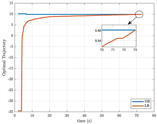
Figure 2.
Trajectory of the bounds yielded by the Benders decomposition solution, for problem and .
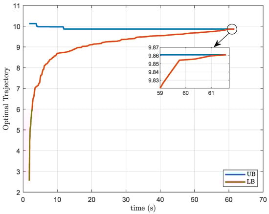
Figure 3.
Trajectory of the bounds induced by the Outer Approximation solution, for problem and .
Another interesting aspect can be observed by analyzing the convergence of both methods for varying length T of predictions horizons. Figure 4 illustrates the slow convergence of the Benders Decomposition, especially regarding the lower bound. Figure 5 illustrates the convergence of Outer Approximation, where slower convergence can also be noticed regarding the lower bound.
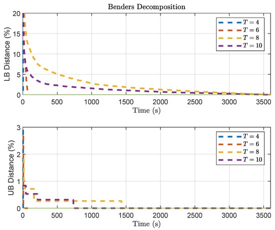
Figure 4.
Trajectory of the bounds in Benders Decomposition solution, for problem , considering a varying length of T for the prediction horizon.
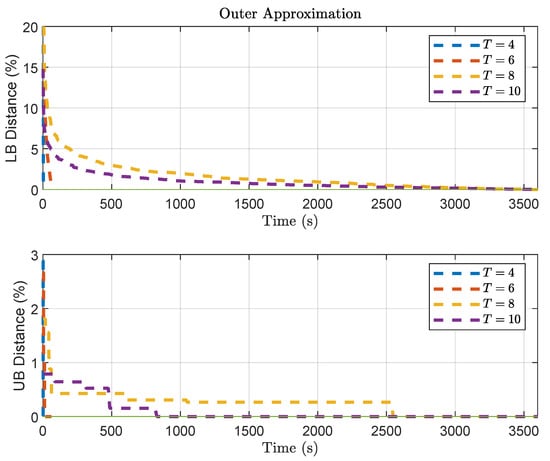
Figure 5.
Trajectory of the bounds in Outer Approximation solution, for problem , considering a varying length of T for the prediction horizon.
Overall, in a set of test problems, both decompositions were able to obtain nearly optimal and globally optimal solutions, with Outer Approximation having a better performance and achieving the global optimal faster than Benders Decomposition for the synthetic problems proposed. Benders decomposition had a lower performance with problems with more subsystems or higher horizons compared to Outer Approximation. However, the results show that the decomposition algorithms produce iterates converging to the same global optimum obtained by their centralized counterpart.
Finally, the results reported in the experiments show that both decomposition strategies can be effective. They allowed the baseline MPC problem to be decomposed into a set of subproblems, whereby the master handles the binary variables (for the activation of control signals) and resource allocations, whereas the subproblems consist of small quadratic programs. The decompositions enabled a distributed solution of the MPC problem to achieve nearly optimal solutions for a given small tolerance. In other words, both hierarchical decomposition formulations can be directly applied to energy management problems under limited resources. The next subsection illustrates the application of the framework to a battery charging problem in electric vehicles.
4.2. Batteries Charging with Activation Constraints
This subsection presents an example problem of charging batteries to illustrate the use of the presented decompositions with activation constraints. Consider an electric car charging station, where each car is represented by an independent system subproblem that reports to the central station master to allocate resources. For each vehicle, there is a state of charge () associated with its battery, which can be defined as in [42]:
in which refers to the current applied at the instant k which, depending on its sign, determines whether the battery is charging or discharging, which also influences the value of which defines battery charging efficiency; sets the battery charge capacity to , and varies within the range (from depleted to fully charged). The structure of the battery charging station and the system behavior are illustrated in Figure 6.
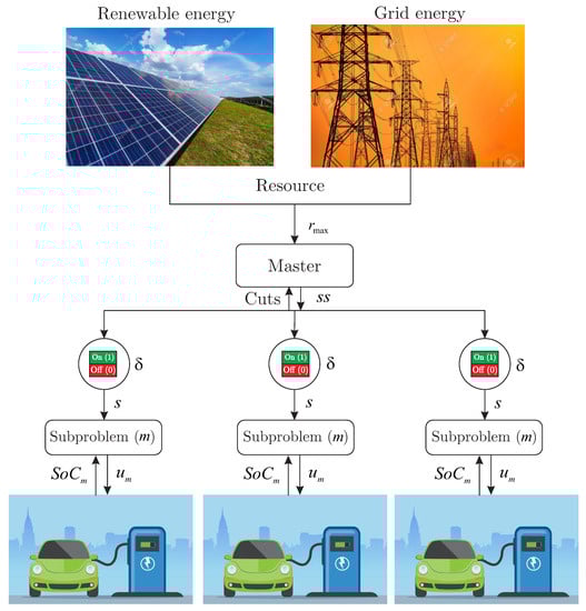
Figure 6.
Distributed MPC for electric vehicle battery charging.
The MPC problem (17) with limited resource constraints can thus be employed in the management of battery charging, using the model given by Equation (30). Problem P, in order to demonstrate a practical application, can be recast as follows:
where:
- is the state of charge prediction for time calculated with the information available until time k;
- is the desired SoC trajectory;
- is the predicted current to be applied to the battery for charging in [A] and is the predicted current variation;
- is the battery charge capacity of vehicle m given in [Ah];
- is the activation variable used for turning the subsystems on/off;
- and are positive definite matrices that penalize the errors on trajectory tracking and control variation, respectively;
- and are known values with the initial conditions;
In this work, only battery charge is considered, so the current signal is non-negative, and, therefore, the charge efficiency value () is considered constant for all vehicles. As shown in Equation (31b), the system output is the value of the state . Therefore, we assume that the state is observable; otherwise, it would be necessary to apply a state observer or Kalman filter [43].
The objective of the problem defined in (31) is the charging of batteries, and, thus, by defining a reference so that all batteries have of , the reference tracking error and the control effort applied to the subsystems are minimized.
4.3. Application to a Sample Instance
Consider a battery charging problem with the following characteristics, , that is, four vehicles, which have identical batteries with a charging capacity , and a charging efficiency . The sampling time chosen was [min], a prediction and control horizon of samples were considered, the maximum resource was for all instants and vehicles, and the current injection limits and its variations were defined as , , and .
The results of applying Benders Decomposition and Outer Approximation to the battery charging instance are shown in Figure 7 regarding the control signals and in Figure 8 regarding the state-of-charge of the batteries. It is possible to notice that all subsystems (vehicle batteries) were charged independently, using the distributed formulation and respecting the maximum available resource and the limits imposed on the defined variables.
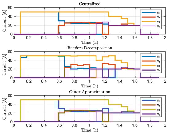
Figure 7.
Control signals applied to the systems.
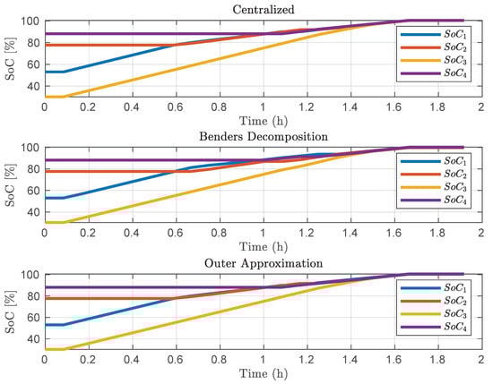
Figure 8.
State-of-charge of the vehicles.
The control actions favored the systems with less , causing them to recharge first. Only after reaching a higher , the control actions direct the available current to vehicles with a higher at the start of charging. The behavior induced by the controller keeps a balance between the resource available and the of all vehicles, thereby achieving the primal goal of charging all cars fully. The analysis showed that the electric vehicles can be recharged in a distributed fashion, approaching the optimal behavior that is achieved by a centralized counterpart.
The fact that the control actions show a similar behavior corroborates with the numerical results presented in Section 4.1, where it can be seen that both formulations manage to converge to a global minimum within a predefined tolerance. Although the Benders Decomposition and Outer Approximation have slightly different behaviors along the charging path, it is expected that they reach close points due to the search for the global optimum. This similar behavior can also be noticed in Figure 9, where it can be seen that the objective value of the cost function is equivalent between the approaches along the iterations of the MPC.
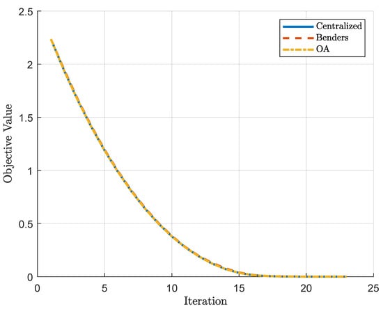
Figure 9.
Objective value for the different approaches along the iterations of the MPC.
5. Conclusions
In this paper, we presented hierarchical decompositions for MPC of resource-constrained dynamic systems with activation constraints on the manipulated variables. First, the MPC problem was cast in a centralized form. Then, Outer Approximation and Benders Decomposition methods were developed for the baseline problem, which was reformulated into a hierarchical structure according to each decomposition strategy. Numerical experiments were performed, in synthetic instances, with the purpose of analysis and to give insights into the efficiency of such decompositions at solving the MPC problem in a distributed distributed fashion.
Considering a set of test problems, both decompositions could obtain nearly optimal and globally optimal solutions, with Outer Approximation achieving a better performance and reaching the global optimum faster than Benders Decomposition. Benders decomposition had a lower performance, particularly in problems with more subsystems or longer horizons, when compared to Outer Approximation. However, the results showed that decomposition strategies produce iterates that converge to the same global optimum achieved by their centralized counterpart.
An application to battery charging of electric vehicles, using activation constraints, was reported using these decompositions methods. The results show that the recharging of electric vehicles can be coordinated in a distributed fashion, approaching the optimal behavior achieved by a centralized controller. The problem’s hierarchical structure makes Benders Decomposition and Outer Approximation ideal for intelligent and distributed control, which are typical of smart systems.
As future work, regularization strategies can be considered for Benders decomposition to increase convergence speed. Multi-cuts can be designed for both decomposition strategies to improve the lower bounds produced by the master problem. In addition, on the application side, the proposed hierarchical frameworks can be applied to other energy systems, possibly considering real data.
Author Contributions
Conceptualization, P.H.V.B.d.S. and E.C.; methodology, P.H.V.B.d.S., L.O.S., and E.C.; software, P.H.V.B.d.S. and L.O.S.; validation, P.H.V.B.d.S.; writing—original draft preparation, P.H.V.B.d.S. and L.O.S.; writing—review and editing, E.C., V.R.Q.L., and G.V.G. All authors have read and agreed to the published version of the manuscript.
Funding
This research was funded in part by the Coordenação de Aperfeiçoamento de Pessoal de Nível Superior, Brasil (CAPES)—Finance Code 001 and supported by the project PLATAFORMA DE VEHÍCULOS DE TRANSPORTE DE MATERIALES Y SEGUIMIENTO AUTÓNOMO—TARGET SA063G19 and Fundação para a Ciência e a Tecnologia—FCT Portugal under Project UIDB/04111/2020.
Acknowledgments
The authors also acknowledge the collaboration of Computer Lab 7 of Instituto de Telecomunicações—IT Branch Covilhã.
Conflicts of Interest
The authors declare no conflict of interest.
Abbreviations
The following abbreviations are used in this manuscript:
| BD | Benders Decomposition |
| DMC | Dynamic Matrix Control |
| EV | Electric Vehicles |
| GPC | Generalized Predictive Control |
| HVAC | Heating, Ventilation, and Air Conditioning |
| lb | lower bound |
| MILP | Mixed-Integer Linear Programming |
| MIMO | Multiple Inputs Multiple Outputs |
| MINLP | Mixed-Integer Nonlinear Programming |
| MPC | Model Predictive Control |
| NLP | Nonlinear Programming |
| OA | Outer Approximation |
| PRP | Production Routing Problem |
| QP | Quadratic Programming |
| SC | Supply Chain |
| SISO | Single Input-Single Output |
| SoC | State-of-Charge |
| ub | upper bound |
References
- Scherer, H.; Pasamontes, M.; Guzmán, J.L.; Álvarez, J.D.; Camponogara, E.; Normey-Rico, J.E. Process Control Efficient Building Energy Management Using Distributed Model Predictive Control. J. Process. Control. 2013, 24, 740–749. [Google Scholar] [CrossRef]
- Scherer, H.; Camponogara, E.; Normey-Rico, J.E.; Álvarez, J.D.; Guzmán, J.L. Distributed MPC for resource-constrained control systems. Optim. Control. Appl. Methods 2015, 36, 272–291. [Google Scholar] [CrossRef]
- Conte, E.; Mendes, P.R.C.; Normey-Rico, J.E. Economic Management Based on Hybrid MPC for Microgrids: A Brazilian Energy Market Solution. Energies 2020, 13, 3508. [Google Scholar] [CrossRef]
- Morato, M.M.; Mendes, P.R.; Normey-Rico, J.E.; Bordons, C. LPV-MPC fault-tolerant energy management strategy for renewable microgrids. Int. J. Electr. Power Energy Syst. 2020, 117. [Google Scholar] [CrossRef]
- de Andrade, G.A.; Mendes, P.R.; García-Clúa, J.G.; Normey-Rico, J.E. Control of a grid assisted PV-H2 production system: A comparative study between optimal control and hybrid MPC. J. Process Control. 2020, 92, 220–233. [Google Scholar] [CrossRef]
- Camacho, E.F.; Bordons, C. Model Predictive Control, 2nd ed.; Springer: Berlin/Heidelberg, Germany, 2007. [Google Scholar] [CrossRef]
- Sandell, N.J.; Varaiya, P.; Athans, M.; Safonov, M. Survey of decentralized control methods for large scale systems. IEEE Trans. Autom. Control 1978, 23, 108–128. [Google Scholar] [CrossRef]
- Colson, B.; Marcotte, P.; Savard, G. An overview of bilevel optimization. Ann. Oper. Res. 2007, 153, 235–256. [Google Scholar] [CrossRef]
- Guignard, M.; Kim, S. Lagrangean decomposition: A model yielding stronger Lagrangean bounds. Math. Program. 1987, 39, 215–228. [Google Scholar] [CrossRef]
- Geoffrion, A.M. Generalized Benders Decomposition. J. Optim. Theory Appl. 1972, 10, 237–260. [Google Scholar] [CrossRef]
- Duran, M.A.; Grossmann, I.E. An outer-approximation algorithm for a class of mixed-integer nonlinear programs. Math. Program. 1986, 36, 307–339. [Google Scholar] [CrossRef]
- Camponogara, E.; Scherer, H.; Biegler, L.; Grossmann, I. Hierarchical decompositions for MPC of resource constrained control systems: Applications to building energy management. Optim. Eng. 2020, 1, 1–26. [Google Scholar] [CrossRef]
- Silva, P.H.V.B.d.; Brinhosa, A.F.; Camponogara, E.; Seman, L.O. A computational analysis of a bilevel decomposition for MPC of resource constrained dynamic systems. In Proceedings of the Anais do 14° Simpósio Brasileiro de Automação Inteligente, Ouro Preto, Brazil, 27–30 October 2019. [Google Scholar] [CrossRef]
- Grossmann, I. Review of Nonlinear Mixed-Integer and Disjunctive Programming Techniques. Optim. Eng. 2002, 3, 227–252. [Google Scholar] [CrossRef]
- Normey-Rico, J.E.; Camacho, E.F. Control of Dead-Time Processes; Advanced Textbooks in Control and Signal Processing; Springer: London, UK, 2007. [Google Scholar] [CrossRef]
- Cutler, C.R.; Ramaker, B.L. Dynamic matrix control: A computer control algorithm. In Proceedings of the Joint Automatic Control Conference, San Francisco, CA, USA, 13–15 August 1980; Number 17. p. 72. [Google Scholar]
- Clarke, D.W.; Mohtadi, C.; Tuffs, P. Generalized predictive control—Part I. The basic algorithm. Automatica 1987, 23, 137–148. [Google Scholar] [CrossRef]
- Clarke, D.W.; Mohtadi, C.; Tuffs, P. Generalized predictive control—Part II extensions and interpretations. Automatica 1987, 23, 149–160. [Google Scholar] [CrossRef]
- Koehler, L.A.; Seman, L.O.; Kraus, W.; Camponogara, E. Real-Time Integrated Holding and Priority Control Strategy for Transit Systems. IEEE Trans. Intell. Transp. Syst. 2018, 20, 3459–3469. [Google Scholar] [CrossRef]
- Seman, L.O.; Koehler, L.A.; Camponogara, E.; Zimmermann, L.; Kraus, W. Headway Control in Bus Transit Corridors Served by Multiple Lines. IEEE Trans. Intell. Transp. Syst. 2019, 1–13. [Google Scholar] [CrossRef]
- Mendes, P.R.D.C.; Normey-Rico, J.E.; Alba, C.B. Economic energy management of a microgrid including electric vehicles. IEEE PES Innov. Smart Grid Technol. Lat. Am. 2016, 869–874. [Google Scholar] [CrossRef]
- Mendes, P.R.; Isorna, L.V.; Bordons, C.; Normey-Rico, J.E. Energy management of an experimental microgrid coupled to a V2G system. J. Power Sources 2016, 327, 702–713. [Google Scholar] [CrossRef]
- Camponogara, E.; Jia, D.; Krogh, B.H.; Talukdar, S. Distributed model predictive control. IEEE Control Syst. 2002, 22, 44–52. [Google Scholar]
- Jordanou, J.P.; Camponogara, E.; Antonelo, E.A.; Schmitz Aguiar, M.A. Nonlinear Model Predictive Control of an Oil Well with Echo State Networks. IFAC-PapersOnLine 2018, 51, 13–18. [Google Scholar] [CrossRef]
- Mendes, P.R.D.C. Predictive Control for Energy Management of Renewable Energy Based Microgrids. Ph.D. Thesis, Universidade Federal de Santa Catarina, Florianopolis, Brazil, 2016. [Google Scholar]
- Floudas, C.A. Nonlinear and Mixed-Integer Optimization: Fundamentals and Applications; Oxford University Press: New York, NY, USA, 1995; p. 450. [Google Scholar]
- Quesada, I.; Grossmann, I.E. An LP/NLP based branch and bound algorithm for convex MINLP optimization problems. Comput. Chem. Eng. 1992, 16, 937–947. [Google Scholar] [CrossRef]
- Westerlund, T.; Pettersson, F. An extended cutting plane method for solving convex MINLP problems. Comput. Chem. Eng. 1995, 19, 131–136. [Google Scholar] [CrossRef]
- Benders, J.F. Partitioning procedures for solving mixed-variables programming problems. Numer. Math. 1962, 4, 238–252. [Google Scholar] [CrossRef]
- Shekarabi, S.A.H.; Gharaei, A.; Karimi, M. Modelling and optimal lot-sizing of integrated multi-level multi-wholesaler supply chains under the shortage and limited warehouse space: Generalised outer approximation. Int. J. Syst. Sci. Oper. Logist. 2019, 6, 237–257. [Google Scholar] [CrossRef]
- Shahabi, M.; Unnikrishnan, A.; Boyles, S.D. An outer approximation algorithm for the robust shortest path problem. Transp. Res. Part E Logist. Transp. Rev. 2013, 58, 52–66. [Google Scholar] [CrossRef]
- Gharaei, A.; Karimi, M.; Hoseini Shekarabi, S.A. An integrated multi-product, multi-buyer supply chain under penalty, green, and quality control polices and a vendor managed inventory with consignment stock agreement: The outer approximation with equality relaxation and augmented penalty algorithm. Appl. Math. Model. 2019, 69, 223–254. [Google Scholar] [CrossRef]
- Rahmaniani, R.; Crainic, T.G.; Gendreau, M.; Rei, W. The Benders decomposition algorithm: A literature review. Eur. J. Oper. Res. 2017, 259, 801–817. [Google Scholar] [CrossRef]
- Colonetti, B.; Finardi, E.C.; de Oliveira, W. A Mixed-Integer and Asynchronous Level Decomposition with Application to the Stochastic Hydrothermal Unit-Commitment Problem. Algorithms 2020, 13, 235. [Google Scholar] [CrossRef]
- Colonetti, B.; Finardi, E.C. Combining Lagrangian relaxation, benders decomposition, and the level bundle method in the stochastic hydrothermal unit-commitment problem. Int. Trans. Electr. Energy Syst. 2020, 30. [Google Scholar] [CrossRef]
- Behnamian, J. Decomposition based hybrid VNS–TS algorithm for distributed parallel factories scheduling with virtual corporation. Comput. Oper. Res. 2014, 52, 181–191. [Google Scholar] [CrossRef]
- Adulyasak, Y.; Cordeau, J.F.; Jans, R. Benders decomposition for production routing under demand uncertainty. Oper. Res. 2015, 63, 851–867. [Google Scholar] [CrossRef]
- Wang, Q.; McCalley, J.D.; Zheng, T.; Litvinov, E. Solving corrective risk-based security-constrained optimal power flow with Lagrangian relaxation and Benders decomposition. Int. J. Electr. Power Energy Syst. 2016, 75, 255–264. [Google Scholar] [CrossRef]
- Bezanson, J.; Edelman, A.; Karpinski, S.; Shah, V.B. Julia: A Fresh Approach to Numerical Computing. SIAM Rev. 2017, 59, 65–98. [Google Scholar] [CrossRef]
- Dunning, I.; Huchette, J.; Lubin, M. JuMP: A Modeling Language for Mathematical Optimization. SIAM Rev. 2017, 59, 295–320. [Google Scholar] [CrossRef]
- Wächter, A.; Biegler, L.T. On the implementation of an interior-point filter line-search algorithm for large-scale nonlinear programming. Math. Program. 2006, 106, 25–57. [Google Scholar] [CrossRef]
- Tudoroiu, R.E.; Zaheeruddin, M.; Radu, S.M.; Tudoroiuv, N. Estimation Techniques for State of Charge in Battery Management Systems on Board of Hybrid Electric Vehicles Implemented in a Real-Time MATLAB/SIMULINK Environment. In New Trends in Electrical Vehicle Powertrains; IntechOpen: Rijeka, Croatia, 2019; Chapter 4; p. 28. [Google Scholar] [CrossRef]
- Kalman, R. A new approach to linear filtering and prediction problems. Trans. ASME J. Basic Eng. 1960, 82, 35–45. [Google Scholar] [CrossRef]


Publisher’s Note: MDPI stays neutral with regard to jurisdictional claims in published maps and institutional affiliations. |
© 2020 by the authors. Licensee MDPI, Basel, Switzerland. This article is an open access article distributed under the terms and conditions of the Creative Commons Attribution (CC BY) license (http://creativecommons.org/licenses/by/4.0/).