Smart Energy Management System of Environmentally Friendly Microgrid Based on Grasshopper Optimization Technique

Abstract

A microgrid is a group of distributed energy resources and interconnected loads that may be operated either in isolated mode or connected mode with the main utility within electrical boundaries. Microgrids may consist of different types of renewable energy resources such as photovoltaic panels, wind turbines, fuel cells, micro turbines, and storage units. It is highly recommended to manage the dependency on these resources by implementing an energy management unit to optimize the energy exchange so that the minimum cost is achieved. In this paper, an energy management system based on the grasshopper optimization algorithm (GOA) is proposed to determine the optimal power generated by the distributed generators in the microgrid which is required to minimize the total generation cost. The proposed unit is applied to a microgrid that consists of five generating units feeding residential, commercial, and industrial loads, and results are compared to other available research in literature to validate the proposed algorithm.

1. Introduction

Lately, the energy resources that are capable of being renewed have been effectively used in the generation of electricity such as the energy that comes from the sun, the offshore wind, biomass, geothermal, etc. In addition, this is a result of the several issues that have an impact on the generation of electricity all over the world in the guise of increasing daily dissipation, causing decrease in the dependence on of the conventional resources of energy, and environmental issues based on them.

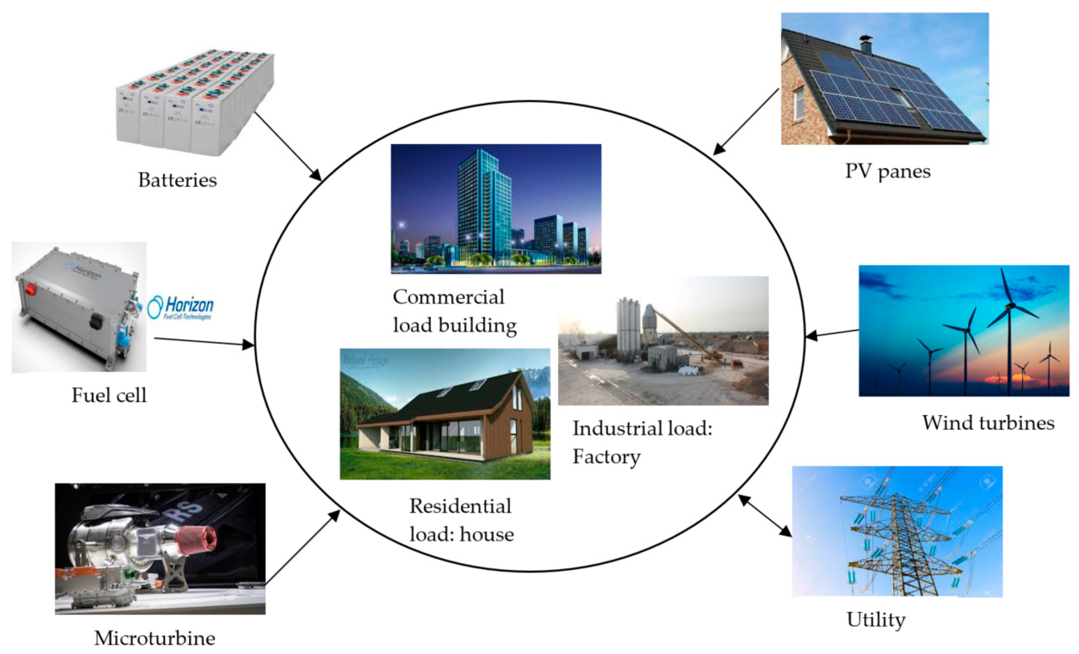
The concept of the microgrid is to coordinate the operation and dominate the distributed generation (DG) sources with the controllable loads as illustrated in Figure 1 [1,2,3,4,5,6,7]. The superfluous energy can be traded off with the grid. Microgrid have been increased all over the world as it could be one of the answers to our energy crisis. It also reduced the transmission losses resulted in transmission of energy especially in remote areas. A high value and trusted energy supply can also be provided by microgrids to critical loads.

Based on the concept of the microgrid, the problem appears in the coordination between different sources of energy along with monitoring the power transfer from the microgrid (MG) to the utility and vice versa as well as the neighboring countries to reduce the generation cost and developing an optimization algorithm to achieve the goal of this paper which is reduction of the generating cost as well as the number of computations.

The formulation of the energy optimization management (EOM) problem in addition to the development of efficient solution methodologies for EOM have been the main concern for many studies. An optimization of real power of different kinds of distributed generators and the power exchange with the main utility network through a centralized microgrid supervision and best operation of it is presented in [2]. The effect of using MGCC with different DG units, storage gadgets, and manageable loads to achieve a well-coordinated operation between them and also achieve the profitable benefits and reduction of the power losses with comparable in the local network is shown in [8]. In [9], a concept of battery lifetime was taken into consideration in establishing an ultimate financial planned style of MG especially when it is linked with the utility. Another kind of algorithm used in fulfilling the required objective which is reducing the cost of the microgrid focusing on the cost of some harmful released gasses as, for example, carbon dioxide, is an adaptive direct search algorithm [10].

Several researchers have used metaheuristics optimization techniques for getting solutions for the energy optimization management with respect to the microgrid.

A matrix real-coded genetic algorithm (GA) is simulated and implemented in [11] to obtain the best operation mode of the MG. In [12], a probabilistic approach established on a GA and two-point estimate technique is provided for solving EOM to diminish the generation cost and maximize the quality of MG which includes PV and wind generation, energy storage, and various loads as ventilation, controllable heating, and air conditioning load. 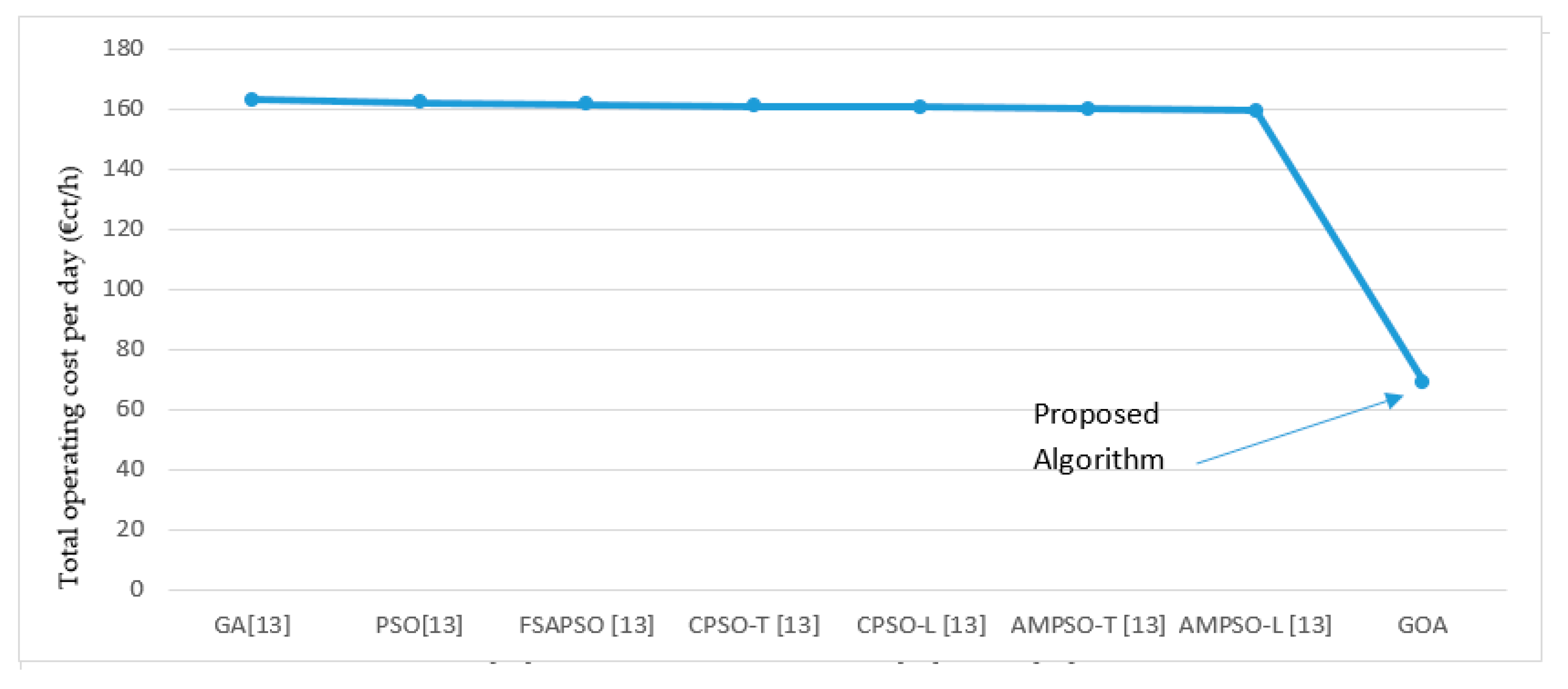According to the several issues related to the operation management of the MG, one of these issues is renewable energy resources joined with backup storage as FC and batteries when it is needed, and this simulated by a modified PSO scheme [13]. A combination based on PSO and optimal power flow is implemented in [14] to examine two different schemes of microgrid with wind farms in common. In [15], the researcher proposed a dynamic technique established mainly on the particle swarm technique for evaluating energy management issues of a MG containing various kinds of distributed generators as well as energy storage equipment. A PSO [16] and imperialistic competitive algorithm [17] were proposed by the researchers in order to settle the ultimate best power dispatch issue of several MGs connected with each other to minimize the operation and comparable the outcomes with Monte Carlo simulation technique. A stochastic weight trade-off PSO based backward-forward sweep OPF technique is proposed in [18] by Mohan to get the online optimal plans of DER in MG taking into consideration renewable energy, power trading with the utility, and demand response.

Niknam, Golestaneh, and Malekpour provided a probabilistic technique for obtaining an energy management for a microgrid consisting only of a renewable energy source having imprecise values in the available electrical power of renewable distributed generators units, market prices, and the consumer consumption in [19]. The uncertainties in the MGs were covered by 2 m point estimate methods while a self-adaptive optimization technique relied on the gravitational search method to evaluate OEM of MG [20]. The optimization method based on an adaptive modified firefly algorithm (AMFA) in [21] is implemented to fix the deterministic issue produced by the scenario production method so the uncertainty is connected with the wind and solar power generation, load forecast mistake, and the market price. In [22], Moradi carried out a hybrid optimization technique that combines two varied algorithms together which are the PSO algorithm and the quadratic programming to fulfill the operational organization for administrating the energy in management in MG and to set the best capacity of the Distributed Generations. As it can be noticed from literature, finding new optimization techniques that can further minimize the total generation cost in MG is still one of the main interesting research points that attracts researchers. In this research work, grasshopper optimization method is presented and simulated for solving the EOM problem of a given MG and this will be discussed in detail in Section 2. In Section 3, the details of the grasshopper optimization technique are provided in addition to the application of the implemented algorithm in the sector of electrical generation. The implementation and results of the applied system are introduced in Section 4. Section 5 provides the conclusion of the paper.

2. Energy Management of Microgrids

2.1. Overview of Microgrids

Due to the geographical and meteorological conditions, the usage of renewable energy distributed generation such as photovoltaic panels and wind turbines faces some difficulties as their generation output is time changeable and their forecasting values are very complicated to be determined. While, the traditional energy sources such as fuel cells (FC), diesel generator (DE), gasoline, micro turbines, and the energy storage equipment can be linked through any point on the grid. In general, microgrid provides the amelioration of the power fineness, reduction the wastage power, reduction of the emissions, and enhancement the system reliability only if it is properly planned and controlled. To achieve the maximum benefit from the MG, the entire DGs unit operation must be well coordinated and controlled with each other and with the storage equipment, as well as the loads, and the operation can be planned during the day. From this point of view, the notion of the microgrid is declared. The classification of the components integrated in a MG is split into two sectors as follows: distributed energy resources as well as the loads. Firstly, the distributed energy sources are divided into dispensed, both of power generators and energy storage systems. The distributed generation is divided into non-renewables sources based on diesel and gas, such as fuel cell and gas turbines, and the renewable dispensed power production from renewable energy sources as sun and wind, such as photovoltaic panels and wind turbines, respectively. While the distributed storage systems are classified according to the application in the short term which provides high power for short period applications, such as super capacitors and long term applications which ensure energy during long periods, such as batteries. Secondly, the loads that are classified as non-controllable or critical load require reliable power supply such as hospitals and military installations and controllable loads that can be scheduled at different times a day.

According to the above information, we can conclude the definition of the MG as a local distribution network that includes various types of dispensable generators, loads whose operation can be well planned during a day and energy storage equipment, which can operate either isolated or interconnected with the upstream network. In the recently developed power systems, the microgrid acts as a principle element in the smart networks.

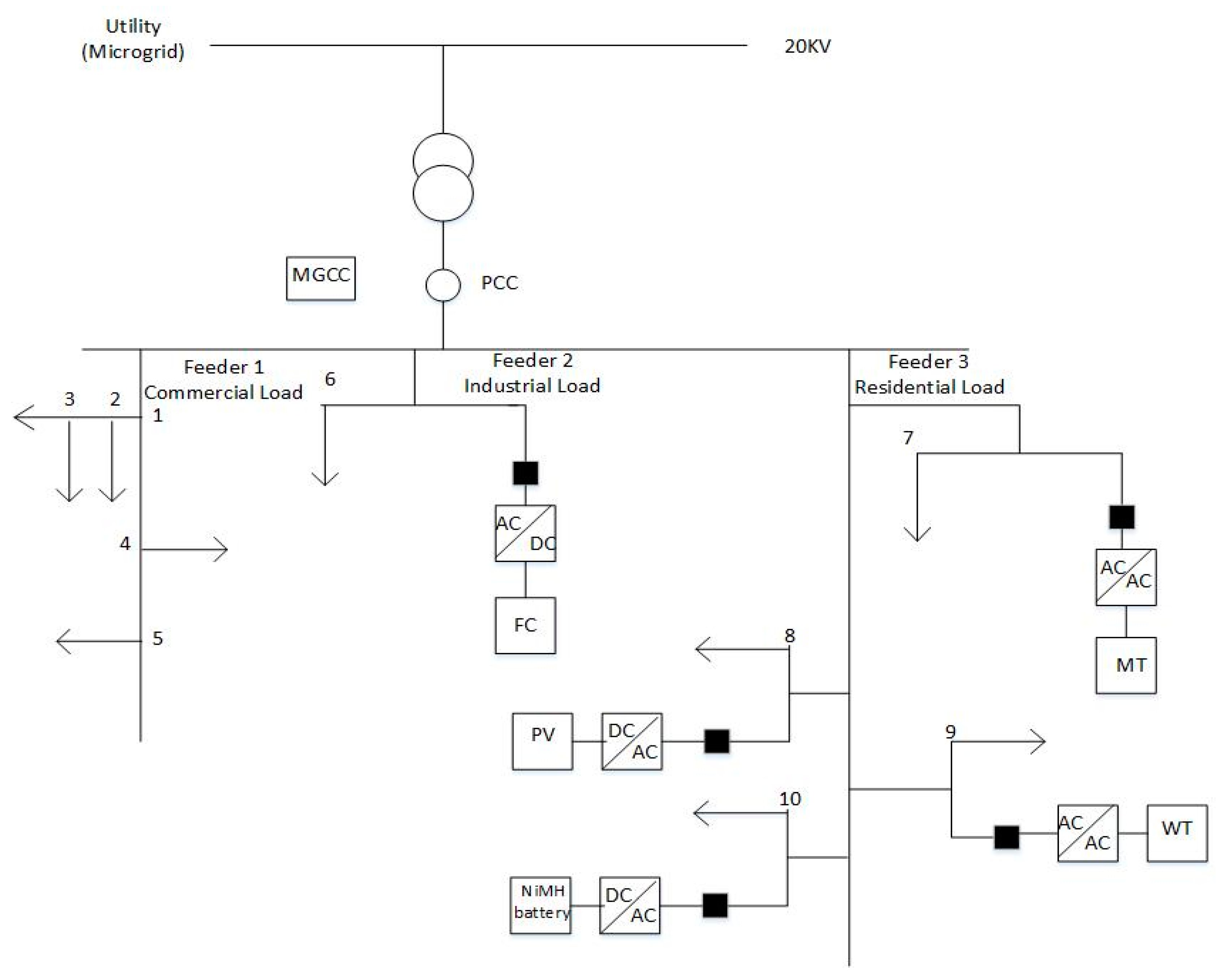
To fulfill the advantages of the operation of microgrid in Figure 2 [1], such as decreasing the operation cost and the less reliance on the upstream network, it is remarkable to merge distributed generators into the microgrid with the upstream network.

Normally, a control framework of any microgrid consists of three hierarchical control degrees [1,2,3,4,5] which are local control (LC), microgrid central controller (MGCC), and distribution management systems (DMS).

Firstly, local management is responsible to control an individual DG unit in the MG as it makes use of nearby data to monitor the voltage and frequency in case of isolated operation mode and in case of interconnection with the main utility it follows the MGCC and performs local optimization. Secondly, the MG central controller acts as a mediator between the MG and the remaining elements in the power network. It monitors both the real power and the power that returns from the load to the upstream network of the distributed generators, in addition, maximizing NG’s value and optimizing its operation. Finally, distribution management systems (DMS) communicate with the MGCC to ensure the system reliability for a safe operation of the MG in the existence of more than one MG.

In general, and from the previous information, we can conclude that the energy optimization management is one of the greatest optimization troubles of the microgrid.

In case the MG is connected to the grid, the microgrid supervision systems can be categorized as centralized and decentralized depending on the decision-making scheme. The centralized management aims to maximize the nearby generation according to the market price by means of a way of communication between both microgrid central controller and nearby controllers. On the other hand, the rendering of the microgrid is getting better in the case of the decentralized control, at which the nearby controllers act in a smart fashion in contact with each other [3]. The MG can trade the excess of energy with the main utility through the distributed management system and the MGCC. The MGCC optimizes the operation of the microgrid with respect to the forecast load, open market prices, tenders received by the distributed generators, and sends signals to the local control of DG sources to be obliged. The applied optimization execution in the microgrid central controller relies on the market policy adopted in the operation of the microgrid.

In this work, the market policy that will be considered in solving the EOM problem states that the prime goal of the microgrid central controller is to supply the total requirements of the microgrid using the nearby generation without releasing power to the upper stream. According to this policy, the tender of the distributed generators, need of the consumption, and the open market prices are essential factors for the central controller in reducing the generation cost.

2.2. Problem Formulation

Based on what we discussed before in this section and as illustrated in Figure 2, the utility provides a generation power to the microgrid through the MV/LV transformer. Both MGCC and the nearby controllers are meaningful for getting the best operation mode of the MG relying on the open-market prices, tenders of the DGs units, and the forecast loads. The best operation of the MG relying on the market policy is simulated in the MGCC. Based on this work, the total consumption of the MG is supplied by its production with limiting the release of energy to the upstream network as much as possible. In this research, a new technique which is GOA is simulated and implemented to reduce the total generation cost through the best modification of the distributed generators while achieving the system constraints.

The mathematical scheme of this issue can be expressed as follows:

2.2.1. Fitness Function

$$mi{n}_x F=mi{n}_x{{\displaystyle \sum }}_{t=1}^{T}cos{t}^t(x^t, y^t )=mi{n}_x{{\displaystyle \sum }}_{t=1}^T{{\displaystyle \sum }}_{i=1}^{TG}[B_{GENi}\left(P_{GENi}{}^t\right)+M{P}^t*P_{Grid}^t$$

(1)

where $x^t$ and $y^t$ are the vector of control variables and dependent variables, respectively. T is the overall time in hours in a given period, TG is the overall distributed generators including the storage equipment and $M{P}^t$ is the market price of energy trading between the MG and the upstream network at time t. The control variables include the generation active power and storage devices inside the MG and can be obvious as follows:

$$x^t=\left[P_{GEN1}^t,P_{GEN2}^t,\dots \dots \dots ,P_{GNG}^t \right]$$

(2)

While, the conditioned variable consists of the real power traded from/to the utility:

$$y^t=P_{Grid}^t$$

(3)

The function of the minimizing the operating cost in Equation (1) is a nonlinear characteristic equation in general because the tender of the distributed generators is normally linear or smooth quadratic function [23].

2.2.2. Constraints

The Energy Evenness

In a given MG for each time interval (t), the total consumption of the consumers is supplied by the local generation within the MG. Therefore, the energy evenness constraint is as follows: taking into consideration that the wastage of the real power within the MG is ignored.

$${{\displaystyle \sum }}_{i=1}^{NG}{P}_{GENi}^t + P_{Grid}^t = {{\displaystyle \sum }}_{D=1}^{TD}{P}_{LD}^t$$

(4)

where $P_{LD}^t$ is a number of the D-th that is the sector of the load, TD is the overall of load sectors.

Computation of the Real Power Bought from or Sold to the Grid

The real power is sold from/to the upstream network to implement the constraints in the real power in Equation (5). The power of the grid is calculated as follows:

$$P_{Grid}^t = {{\displaystyle \sum }}_{D=1}^{ND}{P}_{LD}^t - {{\displaystyle \sum }}_{i=1}^{NG}{P}_{GENi}^t$$

(5)

The variable $P_{Grid,lim}^t$ is defined as follows to satisfy the constraints defined in Equation (6):

$$P_{Grid,lim}^t=\{\begin{array}{c}{P}_{Grid,max}^t, P_{Grid}^t>P_{Grid,max}^t\\ P{ }_{Grid,min}^t, P_{Grid}^t<P_{Grid,min}^t\\ P_{Grid}^t, P_{Grid,min}^t\le P_{Grid}^t\le P_{Grid,max}^t\end{array}$$

(6)

Worth mentioning is that the control variables are self-constrained even as the structured variables have to be introduced to the fitness function as a quadratic forfeiture term and ignoring any illogical solution while the operation process is taking a place. Therefore, the fitness function is updated to be expressed as follows:

$$mi{n}_x F = mi{n}_x{{\displaystyle \sum }}_{t=1}^{NT}cos{t}^t(x^t, y^t ) + {ג}_p{( P_{Grid}^t - P_{Grid,lim}^t)}^{²}$$

(7)

where ${ג}_p$ is the penalty factor.

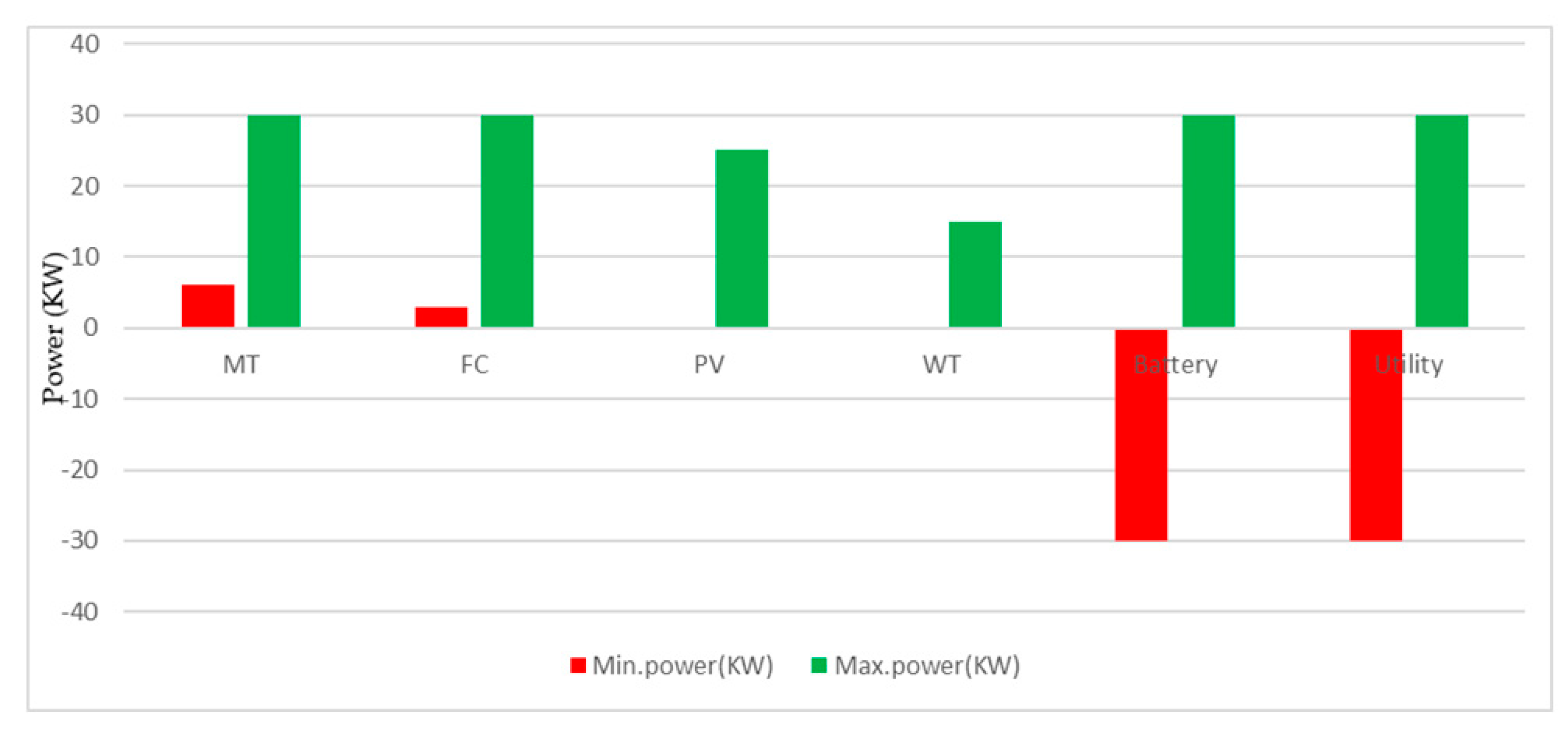
Real Capacity of the Power Production

Each equipment within the MG as well as the utility have their power limitations as follows:

$$P_{GEN{i}_{min}}^t \le P_{Gi}^t \le P_{GEN{i}_{max}}^t$$

(8)

$$P_{Gri{d}_{min}}^t \le P_{Grid}^t \le P_{Gri{d}_{max}}^t$$

(9)

where $P_{GEN{i}_{min}}^t$ and $P_{GEN{i}_{max}}^t$ are the limitations of real power of each distributed generator in a given microgrid at time (t), respectively. While, the $P_{Gri{d}_{min}}^t$ and $P_{Gri{d}_{max}}^t$ are the limitations of real power of the utility at time (t).

Reserve Capacity

To increase the system reliability and to cover the fluctuations in the generation of the renewable energy sources and the load among the time, the spinning reserve is necessary in the MG and the following constraint should be satisfied [15,16,17,18,20,21,24,25]:

$${{\displaystyle \sum }}_{i=1}^{NG}{P}_{GEN{i}_{max}}^t + P_{Gri{d}_{max}}^t \ge {{\displaystyle \sum }}_{i=1}^{NG}{P}_{GENi}^t + P_{LD}^t + R^t$$

(10)

where $R^t$ is the schedule reserve capacity at time (t).

The capacity reserve is an expression that refers to adding an additional value of power to the already existence consumption to fulfil a safety factor supplied for this load.

Energy-Storage Limits

Due to the lifetime of the storage devices, the following expression for a storage device as a battery is obvious as follows [13]:

$$W_{ess,t} = W_{ess,t-1} + {\xi }_{charge}\ast P_{charge}\ast \Delta t - \frac{1}{{\xi }_{discharge}}\ast P_{discharge}* \Delta t$$

(11)

$$W_{ess,min} \le W_{ess,t} \le W_{ess,max}$$

(12)

$$P_{charge} \le P_{charge,max}$$

(13)

$$P_{discharge} \le P_{discharge,max}$$

where $W_{ess,t}$ and $W_{ess,t-1}$ represent how much energy is stored within a given battery at time (t) and (t − 1), respectively, $P_{charge}$ and $P_{discharge}$ are the authorized rate of charge and discharge at a specific period of time ($\Delta t$),${\xi }_{charge}$ and ${\xi }_{discharge}$ are the efficiencies of the battery during charge and discharge processes, $W_{ess,min}$ and $W_{ess,max}$ represent the limitation of the how much energy is stored within the battery, and $P_{charge,max}$ and $P_{discharge,max}$ are the maximum charging and discharging rate of the battery during each time interval $\Delta t$.

2.2.3. Distribution Generation Bid Calculation

The market prices and a fulfill profit are deemed to be important outcomes of using a MG especially when it is connected to the upstream network. These outcomes are based on the distributed generators from the point of their cost function [8]. The tender of the distributed generators is seen to be a quadratic function as follows:

$$B_{GENi}= a_i\ast \left(P_{GENi}{}^2\right)+b_i\ast P_{GENi}+ c_i$$

(14)

Micro-Turbine and Fuel Cell

The computation of the tender of the distributed generators of both micro-turbines and fuel cells can be obtained through the following equation [10,26]:

$$B_G= C_{fuel}\ast \frac{P_G}{{\xi }_G}+ C_{inv} \left(€/\mathrm{h} \right)$$

(15)

where $C_{fuel}$ is the price of fuel used to outfit distributed generators in $\left(€/\mathrm{KW} \mathrm{h} \right)$, $C_{inv}$ is the development cost resulted from its quantity of redeem each hour a day $\left(€/ \mathrm{h} \right)$, and can be calculated as follows:

$$C_{inv}= AC\ast \frac{P_{Gnom}}{AP}\left(€/h \right)$$

(16)

$$AC= \frac{i{\left(1+i\right)}^n}{{\left(1+i\right)}^n-1} \ast IC \left(€/KW -year\right)$$

(17)

where $AC$ and $AP$ are the annual investment cost and annual production cost, respectively, $P_G$ is the generated power of the distributed generators in (KW), ${\xi }_G$ is the efficiency of the electric DG unit, (i) is the annual percentage rate, (n) is the consumption in interval of time in years, and IC is the cost of structure of each equipment with a given microgrid.

The efficiency of the micro turbines is boosted in respect to generation output power and its characteristics can be predestined as a quadratic function of its generated power [27]. On the other hand, the efficiency of the fuel cell can be evaluated through a nonlinear function of power level [28].

Diesel Generator

The power rating in KW of the distributed generators are based on the information of the exhaustion of the diesel-fuel with respect to each manufacturer. The features of this exhaustion for each diesel generator are obvious as a quadratic function of its generated real power.

$$Fue{l}_{DE}= a_f\ast \left(P_{DE}{}^2\right)+b_f\ast P_{DE}+ c_f$$

(18)

where $Fue{l}_{DE}$ is the fuel exhaustion of a given DE in (L/h), $P_{DE}$ is generated power of DE in KW in addition to $a_f$, $b_f$, and $c_f$ that are the degrees of features based on fuel exhaustion. Therefore, the tender of DE $\left(€/\mathrm{h} \right)$ can be simulated as follows:

$$B_G= C_{fuel}\ast Fue{l}_{DE} + C_{inv} \left(€/\mathrm{h} \right)$$

(19)

where the $C_{fuel}$ is the cost $(€/\mathrm{L}$) of the amount diesel-fuel required to outfit the diesel generator.

Wind Turbines and Photovoltaic Panels

First of all, with respect to the wind turbines, the generation power during a year in KW h/KW as well as development cost of the equipment due to its consumption in $\left(€/\mathrm{kw} \right)$ are the factors in determining their tender function which can be expressed through the following equations.

$$B_G= \frac{AC}{AP} \ast P_G\left(€/h \right)$$

(20)

$$AC= \frac{i{\left(1+i\right)}^n}{{\left(1+i\right)}^n-1} \ast IC \left(€/h \right)$$

(21)

Due to the irregularity of the output power of both WT and PV distributed generators, the predicted generation power of both wind turbines and photovoltaic panels is desired for solving optimization problems.

The speed of the wind in a definite site and its power curve [29] are two essential features in evaluating its generation power which can be cleared in the following equations:

$$P\left(WT\right)=\{\begin{array}{c}0, V\le V_{ci}\\ 0,V>V_{co}\\ P_{nom},V_{nom}<V\le V_{co}\\ \left(\frac{V^2-V_{ci}^2 }{V_{nom}^2-V_{ci}^2 }\right)\ast P_{WT,nom},V_{ci}<V\le V_{nom}\end{array}$$

(22)

where $P_{WT,nom}$ is the nameplate capacity of power, $V_{nom}$ is the speed of wind, $V_{co}$ is the rated wind speed at which the wind turbines can withstand, and finally $V{ }_{ci}$ is the minimum wind speed at which the turbines start to generate power, $P\left(WT\right)$ is the output power of the wind turbines, and $V$ is the speed of the wind.

Secondly, with respect to the photovoltaic panels, the solar irradiance, ambient temperature, and the features of the panels are the essentials parameters in generating its power which can be evaluated through the following equation:

$$P_{PV} = P_{STC}\ast \frac{I_s}{800} [1+Ƴ (T_c-25\left)\right]$$

(23)

where $P_{STC}$ is the ultimate generation power for a given photovoltaic panel with respect to basic situations for its evaluation (W), $(I_s$) is the solar irradiance on the surface of the photovoltaic panel (W/${\mathrm{m}}^2$), (Ƴ) is the degree of temperature for the generation power (°${\mathrm{C}}^{-1}$), $T_c$ is the temperature of the photovoltaic panel (°C) and it can be calculated as follows:

$$T_c = T_a + ( \frac{I_s}{800} ) (T_{NOCT}-20 )$$

(24)

where $T_{NOCT}$ is the nominal operating cell temperature (°C) and $T_a$ is the ambient temperature (°C).

Bids of the batteries are defined by Equation (19).

3. Overview of Grasshopper Algorithm

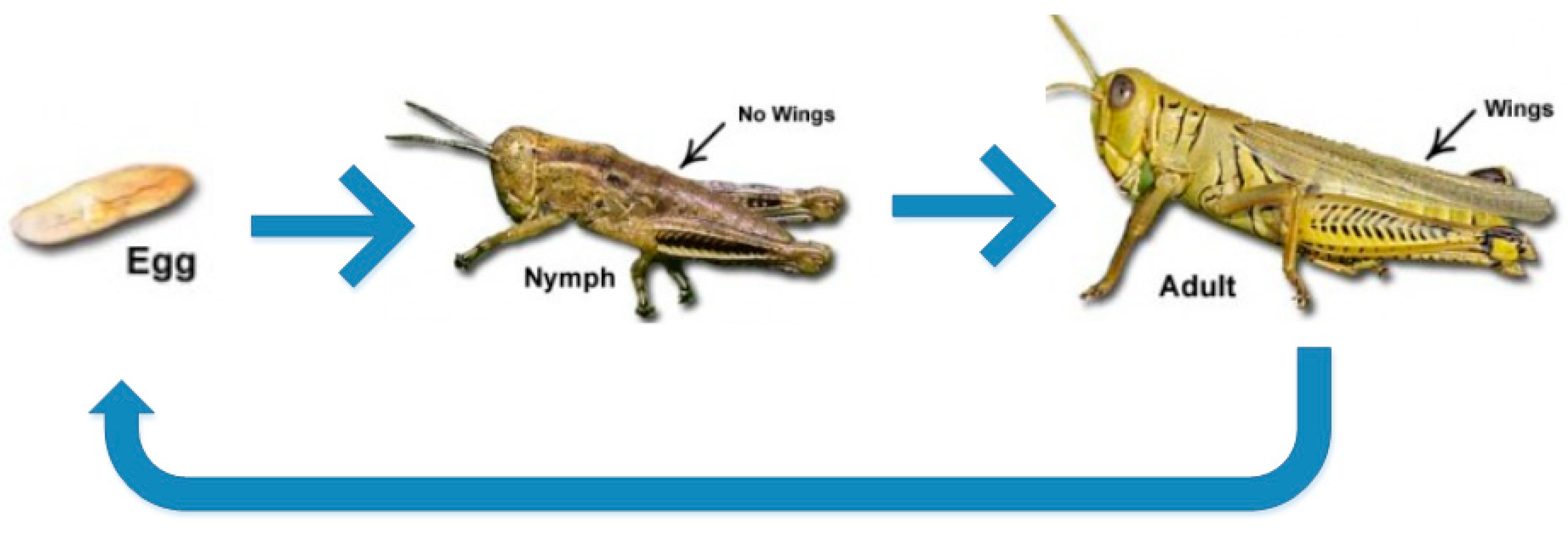
Grasshoppers are insects. They are considered to be harmful insects due to their damage related to diminishing agriculture production. Figure 3 represents the chain of modifications in the life of grasshoppers.

Despite the fact that grasshoppers are ordinarily observed individually, they move and participate in a biggest group among other creatures [30]. The volume of this group may be a nightmare for ranchers. The exceptional part of this group is that its behavior is found in both the nymph and the adulthood [31]. A huge number of nymph grasshoppers bounce and move like trigger clambers. As they trigger around, all of the harvest is eaten. After this behavior and when they become adults, they form a structure of multitude noticeable all around. This is the manner by which the grasshopper evacuates far way.

The fundamental attribute of the herd in the icteric stage is moderate activity and little strides of the grasshopper. Conversely, the most significant merit of this herd is the sudden movement among extended zones in addition to the investigation for the food source. Both exploration and exploitation are two denominations classified by the natural inspired techniques. In the first denomination, the motion of the search agents is observed to be an abrupt motion. Subsequently, the design of the developed inspired technique will be achieved only if we can find a way to make a mathematical model for the behavior of the swarm. The mathematical model of the swarming behavior of the grasshopper is presented as follows [32]:

$$X_n = S_n+ G_n+ A_n$$

(25)

where $X_n$ is the current placement of any of the grasshoppers, $S_n$ is the social interaction, $G_n$ is the gravity force, and $A_n$ shows the wind advection. An imprecise attitude of the herd can be evaluated from the following equation:

$$X_n = r_1{S}_n+r_2 G_n+r_3 A_n$$

(26)

where $r_1$,$r_2$, and $r_3$ are random numbers from [0, 1].

The social interaction ($S_n)$ is obtained through the following equation:

$$S_n= {{\displaystyle \sum }}_{\begin{array}{c}m=1\\ m=ǂn\end{array}}^{N}s\left(dnm\right)d_{mn}^{^}$$

(27)

$\mathrm{where} (d_{nm}$) is the displacement between two nearby grasshoppers and it is evaluated from $d_{nm}$ = |$X_m$− $X_n$|, ($s$) is the function that indicates the vigor of social forces and is calculated as follows:

$$\mathrm{s}\left(\mathrm{r}\right) = \mathrm{f}{e}^{\frac{-r}{l}}-e^{-r}$$

(28)

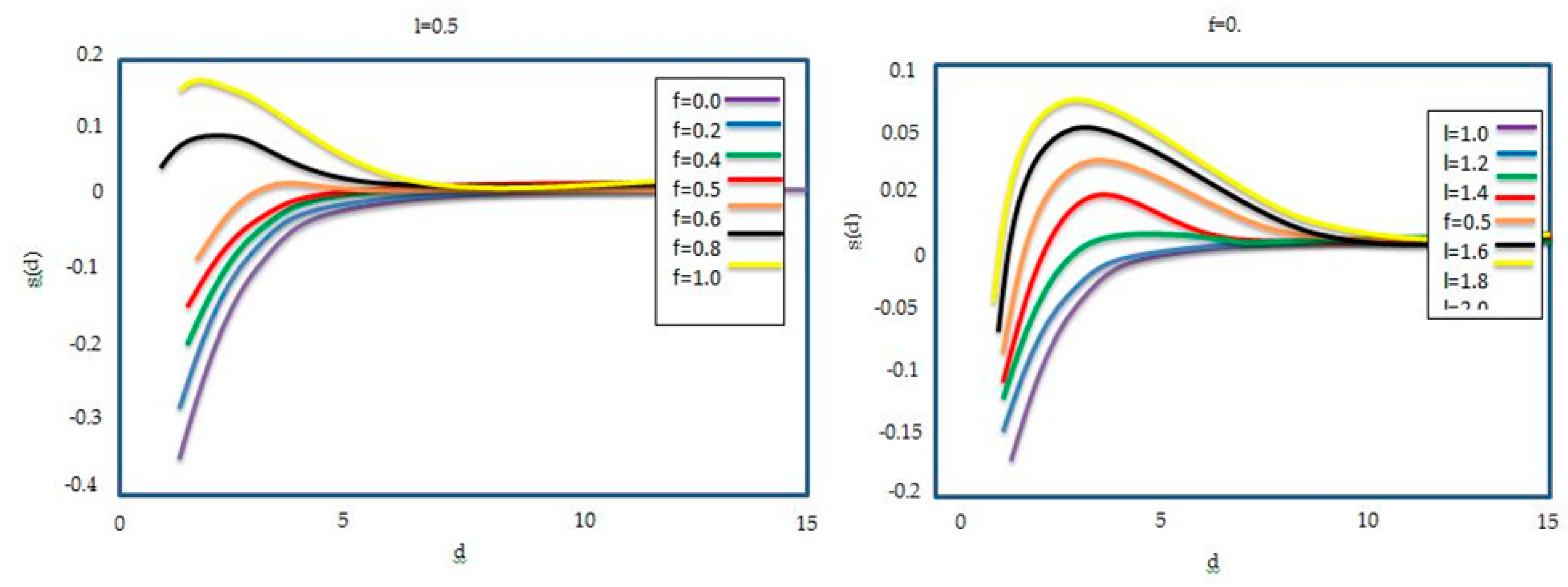
Additionally, the $(d_{mn}^{^}$) is a vector in which its magnitude equals to one displacement and two grasshoppers and be obtained as follows:

$$d_{nm}^{^}= \frac{x_{m-x_n}}{d_{nm}}$$

(29)

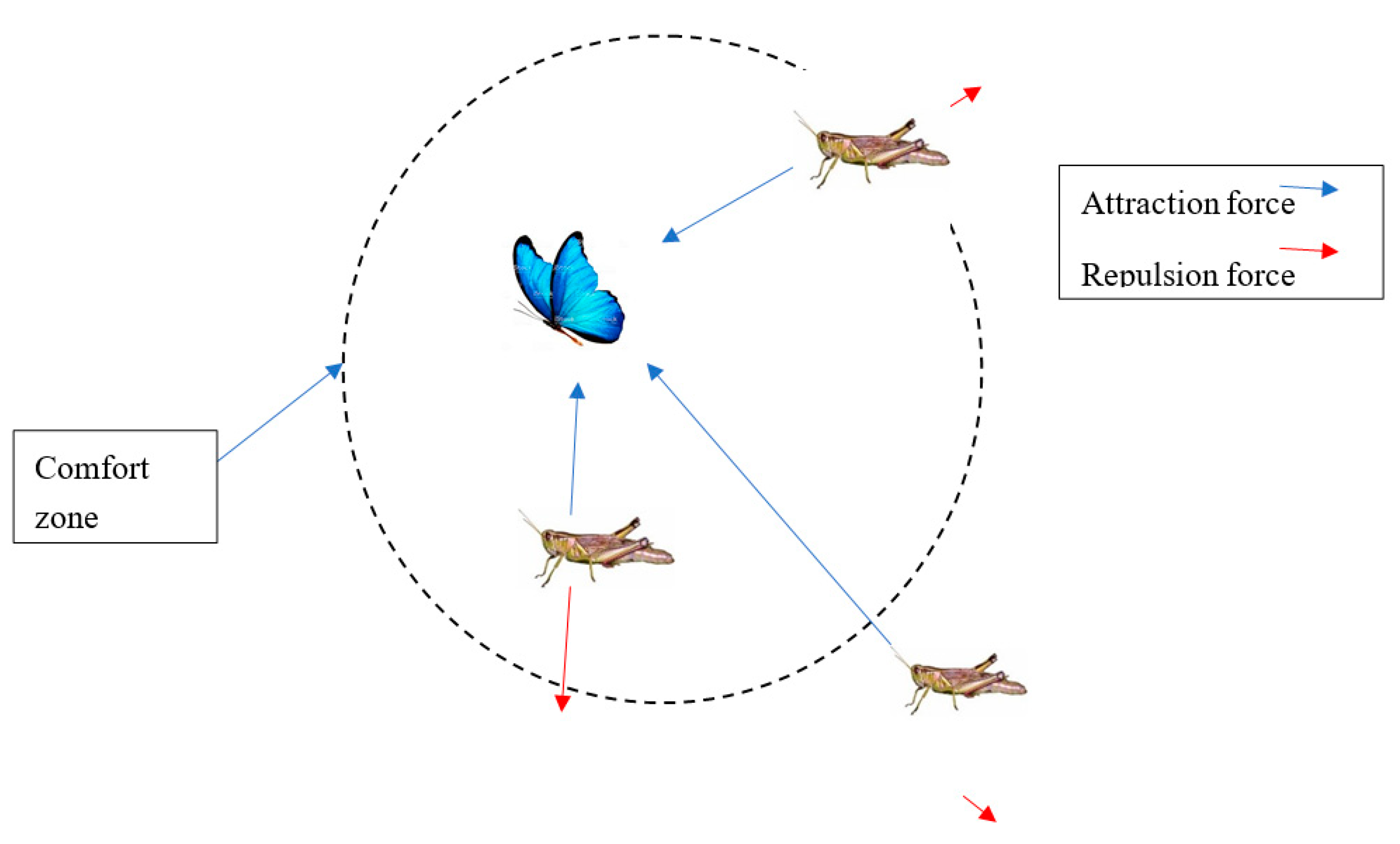
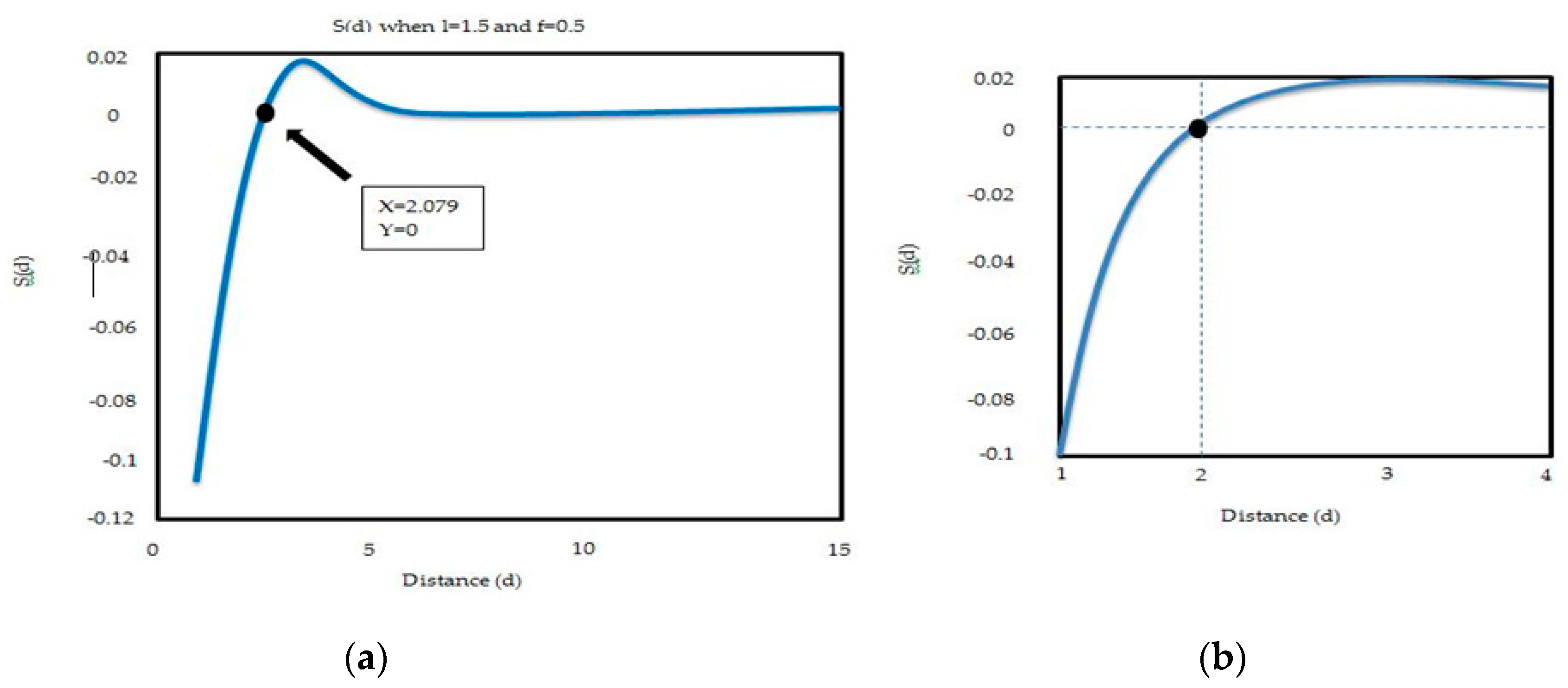
where (f) represents the attraction vigor while (l) is the level of the attractive longitude. The value of (s) is illustrated in Figure 4 showing its impact on the social interaction of grasshoppers. As it is shown in Figure 4a it is obvious that the repulsion between the grasshoppers occurs within interval from 0 to 2.079 with displacement changing from 0 to 15. At 2.079 units far away between two grasshoppers, the attraction and repulsion between them disappear and this is called the comfort zone. In Figure 5, the variation of the two factors (l, f) are considered in plotting the value of (s) in Equation (28). It is noticeable that for a few values of l and f for example 1, 0.5, respectively, both the attraction and repulsion zones are very small. The value of (s) is used to express the relationship between the interaction of grasshoppers and the comfort zone as it shown in shown in Figure 6 [33]. The implementation of (s) has an observable issue in applying strong forces between the individual grasshoppers as its value reaches zero with extended displacements more than 10 between them despite its capability in determining the attraction and repulsion zones. The force of gravity is evaluated from the following:

$$G_n = -\mathrm{g}{e}_g^{^}$$

(30)

where (g) is the gravitational constant and ($e_g^{^}$) shows a unity factor towards the center of the earth. The (A) component in Equation (25) is calculated as follows:

$$A_n = \mathrm{u}{e}_w^{^}$$

(31)

where (u) is a constant drift and ($e_w^{^}$) is a unity vector in the direction of wind. As illustrated before in Figure 3, the wind direction has a significant effect on the nymph grasshoppers as they have no wings. By replacing S, G, and A in Equation (25), the equation can be expressed as follows:

$$X_i={{\displaystyle \sum }}_{\begin{array}{c}m=1\\ mǂn\end{array}}^{N}s\left(\left|x_m-x_n\right|\right)\frac{x_m-x_n}{d_{nm}} - \mathrm{g}{e}_g^{^}+ \mathrm{u}{e}_w^{^}$$

(32)

where N is the number of grasshoppers.

The location of the minor female of the grasshoppers is not allowed to reach a point at which there is a change in the execution of the program, although these grasshoppers can land on the ground. Therefore, the equation entire simulation of this case is never used as it blocked the algorithm from both exploration and exploitation of the search agent around the solution. In conclusion, the implemented scheme of the herd took place in the free space. According to Equation (32), the interaction between the grasshoppers and each other in the swarm is implemented. However, this mathematical model cannot be used directly in solving optimization issues because the grasshoppers reach the comfort zone quickly and the herd does not focus on a nearby special point. Therefore, Equation (32) is modified and proposed as follows to solve the optimization problems:

$$X_m^d= \mathrm{c}[{{\displaystyle \sum }}_{\begin{array}{c}m=1\\ mǂn\end{array}}^{N}c\frac{u{b}_d-l{b}_d}{2}*\mathrm{s}(|x_m^d- x_n^d|)(\frac{x_m-x_n}{d_{nm}})]+T_d^{^}$$

(33)

where $u{b}_d$ and $l{b}_d$ are the upper and lower bounds in the D-th dimensions, respectively.$T_d^{^}$ is the optimal solution so far and (c) is a decreasing degree to contract the attraction zone, repulsion zone, and the comfort zone. The (G) component is neglected and the wind direction is assumed to be always towards the target ($T_d^{^}$). There are three factors in determining the following displacement of a given grasshopper which are its current displacement, the objective displacement, and the locations of the other grasshoppers and this appears in Equation (33). This technique is totally different to that of PSO as we mentioned before in the literature.

In the particle swarm optimization, two essential factors are required to define each particle which are the position and velocity vectors, while in grasshopper optimization (GOA), the search agent is defined by only one displacement vector.

Other factors differentiate between both techniques in determining the displacement of the particles. According to the PSO, the current displacement, the best solution obtained by an individual and the best solution obtained by the swarm are the essential factors in locating the position of particles; while, with respect to the GOA, it is the current location, the superior solution gained by an individual, the best solution obtained by the swarm, and the locations of the other search agents. According to Equation (33) it is clear that the adaptive element (c) has repeated two times for the following reasons:

• The first (c) is nearly comparable to the inertial weight (w) in PSO and it is responsible for remission of the motion of grasshoppers towards its target and this occurs through managing both exploration and exploitation.
• The second (c) aims to reduce the attraction, repulsion, and comfort zones between the grasshoppers.

In respect to Equation (33), it is obvious that the element (c) inside the equation is directly proportional to the number of iterations as it participates in reducing the attraction and repulsion between the grasshoppers. In addition, the outer element (c) plays a role in decreasing the concourse towards the target with increasing the number of iterations.

Finally, and according to Equation (33), the start of this equation represents the location of the other grasshoppers and simulates their interaction in nature. In addition, the second part which is identified by ($T_d^{^}$) simulates its motion capability towards the target.

In general, the grasshoppers tend to stir and look for their food locally as in the icteric phase they have no wings, in the next stage, they scout much larger level zones as they tend to move freely in air. In stochastic optimization techniques, exploration comes first due to the need for finding promising regions of the search space. After finding these regions, exploitation search agents assume to search locally to find the global optimum as an accurate approximation value. The coefficient (c) is calculated as follows:

$$\mathrm{c} = \mathrm{cmax} - \mathrm{i} ( \frac{ \mathrm{cmax}-\mathrm{cmin}}{\mathrm{I}} )$$

(34)

where cmax and cmin are the limitation values, (i) indicates the present iteration while (I) is the ultimate number of iterations. In this work, cmax and cmin are set to be 1 and 0.00004, respectively. In reality, the global optimum solution is not known, so there is no target to achieve it. Therefore, there must be an evident objective for grasshoppers in each step which is the best objective value. This is will aid GOA to keep the most objective value in the search space in each iteration and require grasshoppers to move towards it.

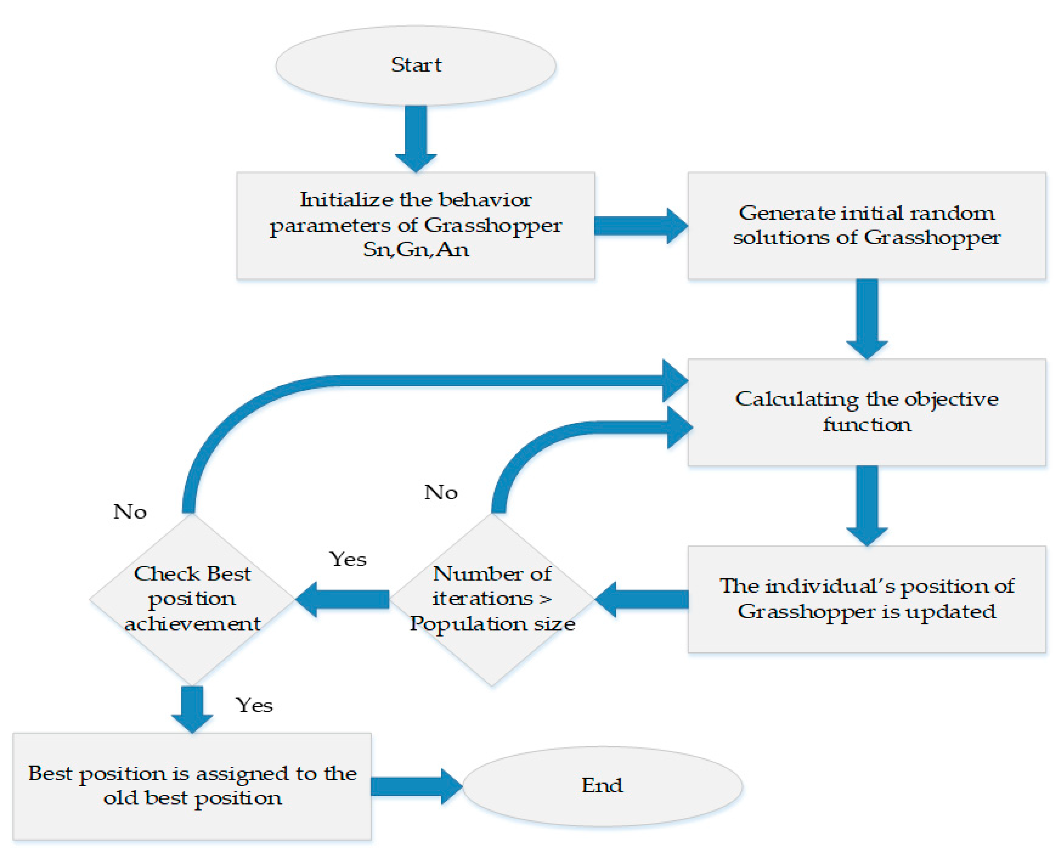
The flowchart of the grasshopper optimization technique is expressed in Figure 7. The GOA starts the optimization by initializing the behavior parameters such as $S_n$, $G_n$, $A_n$, cmax, cmin, etc., then generating random solutions. In addition, the fitness function is evaluated leading to updating the locations of search agents based on Equation (33). The best target position is obtained and updated in each iteration. After that, the number of iterations is compared with population size and if the number of iterations is greater than the population size, then the best position will be observed whether it reaches the best position or not. If not, the fitness function will be evaluated again. Therefore, if the best position is achieved then it will be assigned to the old position and if not, the fitness function will be evaluated. Finally, the location and the objective of the best target is returned as the best approximation for the global optimum.

Application of GOA to EOM

The implementation of the grasshopper technique for solving the best energy optimization management briefly occurs through the following:

• Step 1: Define the configuration of the proposed scheme.
• Step 2: Define the system data including DG units, storage devices, loads, and the control strategy.
• Step 3: Define the active power of DG and the storage units and their limitations (2).
• Step 4: Define the real power traded off with the utility (3).
• Step 5: Define the objective function that is required to be optimized (1) and the penalty factor to form the updated fitness function (7).
• Step 6: Initialize GOA parameters such as the social interaction (S), gravity force (G), the wind advection (A), decreasing coefficient (c), and the ultimate number of iterations (i).
• Step 7: Generate an initial random generation of grasshoppers.
• Step 8: Evaluate the real power traded off with the utility for each search agent in the current population (5) and check their constraints (6).
• Step 9: Evaluate the fitness function for each search agent using (1) and (7).
• Step 10: The individual position of the grasshopper is evaluated according to (25).
• Step 11: The number of the iterations is then compared with the population size.
• Step 12: Check the position achievement.
• Step 13: Repeat steps 9–12 until the best solution is achieved.
• Step 14: Return the optimal solution gained in the last iteration; stop.

4. Simulation and Results

In this work, the simulation and the results of the proposed scheme were utilized to be compared with those referred in the literature based on a standard MG [13,19,21,34] at low voltage level.

The computer used to simulate this proposed scheme has the specifications of a processor with speed 2.60 GHz, a memory of 8 GB ram. All the simulations were carried out on Matlab^®.

The proposed MG in Figure 2 consists of different DGs from renewable and non-renewable sources such as wind turbines (WT), photovoltaic panels (PV), fuel cells (FC), micro turbines (MT), as well as the storage devices like batteries. All of the DGs sources within the proposed MG are assumed to generate real power as well as the load is considered to be purely resistive. In addition, the excess of energy within the MG can be traded off with the utility during a day through a power exchange link based on the data obtained by the MGCC.

The generation limits of the installed DG units as well as its bid coefficients are cleared in Figure 8 and Figure 9 in sequence [13]. These installed DGs units tend to feed a load demand of residential, commercial, and industrial loads with total capacity of 1.695 (KW h) for a given day. The forecast of load demand differs throughout a day according to the user consumption as shown in Figure 10.

While, the predictive values of the market price, maximum available real power of both wind turbines and photovoltaic panels are introduced in Figure 11.

In this simulation and results section, we test the proposed algorithm in two different scenarios as follows:

4.1. First Scenario

As we mentioned before in Section 2, the proposed MG includes various types of the distributed generators, storage devices, and the utility. Each DG unit will be operated according to this scenario as follows: the renewable DGs will produce their ultimate available power each hour a day, while the other DG units, the storage devices, and the utility will produce their power within their generation limits as shown in Figure 12 taking into consideration their constraints. The excess of energy inside the MG will be traded off with the utility.

In addition, the corresponding operating cost for each hour a day for all the elements in the MG is shown in Figure 13. The obtained results from Figure 9 and Figure 12 show that when the bid coefficients of a given DG are lower than the other DGs, the load is then supplied mainly from this DG as it is clear from Figure 12, the periods from 1 to 7 (h) and from 23 to 24 (h) the load is supplied by a fuel cell and the utility such as the market price of the utility in these periods are low, as shown in Figure 11. On the other hand, when the bid coefficient of a given MG is higher than the other DGs, the load is then supplied by the lower one and the excess of energy is exported to the utility as the market prices in these periods is too high as is clear in periods from 8 to 17 (h) and from 21 to 22 (h). It is also clear that the charging process of the batteries occurs in periods at which the market price of the utility is low as from 1 to 6 (h) and from 23 to 24 (h). The resulting overall cost in this scenario is 268.9951 cent/h.

4.2. Second Scenario

In this scenario, all of the DG units in the proposed MG act differently from the previous scenario in the sharing of the generation power. The DGs installed in the proposed MG, the storage devices, and the utility will produce their power within their generation limits taking into consideration their constraints as is clear in Figure 14.

Figure 15 shows the total generation cost for all the MGs components for each hour daily. The significant reduction in the total operating cost in comparison with the first scenario is obvious from Figure 16, and for the lower participation of the photovoltaic panels for the relatively high bid coefficients and a high participation of wind turbines as their bid coefficients is shown in Figure 9, if compared with the other DG units in the proposed MG. While, at high values of the market price as in Figure 10, the output generation of the MT, FC, and the batteries is considered to be at their maximum production and vice versa. Additionally, as in first scenario, the surplus of energy within the MG is traded off with the utility. The obtained overall cost from this second scenario is 69.0924 cent/h

The obtained results from both scenarios were compared with other techniques of solving EOM problems as we mentioned before in literature [13,19]. According to Figure 17 and Figure 18, the proposed grasshopper based algorithm (GOA) proves its efficiency in getting optimal solutions for EOM problems in the two scenarios. In the first scenario, the best obtained result in the literature was equal to 269.76 cent/h by SGSA technique as proposed in [19] and the proposed GOA gave a lower cost of 268.9951 cent/h. In similar manner, the second scenario best result in literature was 159.3628 cent/h at the time the proposed GOA gave a much lower overall cost of 69.0924.

The high convergence rate to reach the optimal solution is clearly shown in Figure 19, which presents a sample solutions for this EOM problem in the 3rd, 12th, and 19th hours, respectively.

4.3. Discussion

4.3.1. Simulation Parameters

It is important to mention that the simulation results were obtained at number of 300 iterations only along with 120 search agents. Where, the maximum execution time for generation cost of a given hour was 121.5 s and this occurred when simulating the first hour, and the minimum time was 88.3 s when simulating the 11th h. The total execution time for the 24 h is approximately 2290 s with average execution time 95 s per h simulated with the desktop computer with specifications mentioned earlier in this section. Although it is very hard to compare execution time with other research in literature without enough information about their execution times, it can still be noticed that GOA may be a successful candidate when it comes to execution speed as it only used 300 iterations to achieve better results in comparison with 1500 iterations for GSA an SGSA as indicated in [19]. More importantly as presented in Section 3 it can be noticed that the proposed GOA algorithm equations have easy mathematics which also may contribute to execution speed. Finally, it is well known that this optimization problem type is offline, which means that execution time would neither affect the real life operation of the system nor the total generation cost achieved.

4.3.2. Theorem Implications

There are three main factors that could have implications of the proposed method:

1-

The first factor is the ability of the grasshopper optimization algorithm (GOA) to avoid falling in local optimum value and this can clearly appear in the results mentioned in this section as it gave in all hours (both cases) best optimized results.

2-

The second factor is the high convergence rate, and this clearly appears in the quick convergence that occurs in both cases as it converges in only 300 iterations as shown in Figure 19.

3-

The third factor is the computational complexity, the GOA has small computational burden especially that although the application of the energy management is considered high dimensional and a complex problem, and the GOA succeeded in solving this problem with only 120 agents.

5. Conclusions

In this paper, a nature inspired technique was used to solve an EOM problem and applied on a standard MG which is the grasshopper optimization algorithm. The MG comprises different types of DG units as well as the loads as we mentioned before in Section 2. Two scenarios were considered in this work. In the first scenario considered, all the DG units, storage devices, and the utility operated within their limits except the renewable DG units which generated their maximum power. While in the second scenario, all of the DG units, storage devices, and the utility operated within their limits taking into consideration their limits and the surplus of energy in both scenarios are traded off with utility. The obtained results from both scenarios were compared with other different optimization techniques available in previous research. The proposed grasshopper optimization algorithm produced lower cost in both scenarios and could efficiently find the optimal solutions for solving EOM.