Abstract
The fundamental harmonic amplitude and waveform distortion rate of the air-gap flux density directly affect the performance of a permanent magnet spherical motor (PMSM). Therefore, in the paper, the axial air-gap magnetic field including the end leakage of the Halbach array PMSM is analyzed and optimized. In order to reduce the calculation time of the objective function, the air gap magnetic field model adopts a non-linear regression model based on support vector machine (SVM). At the same time, the improved grid search (GS) algorithm is used to optimize the parameters of SVM model, which improves the efficiency and accuracy of parameter optimization. Considering the influence of moment of inertia on the dynamic response of the motor, the moment of inertia of the PMSM is calculated. This paper takes the air gap magnetic density fundamental wave amplitude, waveform distortion rate and rotor moment of inertia as the optimization objectives. The particle swarm optimization (PSO) algorithm is used to optimize the motor structure with multiple objectives. The optimal structure design of the PMSM is selected from all of non-dominated solutions by the technique for order preference by similarity to an ideal solution (TOPSIS). The performance of the motor before and after the optimization is analyzed by the method of finite element (FEM) and experimental verification. The results verify the effectiveness and efficiency of the optimization method for the optimal structure designing of the complex PMSM.
1. Introduction
The structure optimization design for a motor is to further improve its performance, such as back-electromotive force (EMF) performance, and torque performance, which is largely influenced by the air-gap magnetic field. A permanent magnet spherical motor (PMSM) has a wide application in multi-degree-of-freedom motion systems such as spacecraft, manipulators, and panoramic cameras because of its small size, light weight, and high torque output [1,2]. In [3], the Halbach magnet array is applied to spherical motors, making the air-gap magnetic field closer to the sinusoidal distribution. However, due to the short axial length of PMSM, the axial air-gap magnetic density shows a rapid attenuation from the equator to the two ends of the permanent magnet (PM), which results in the distortion of the main air-gap magnetic field [4]. Moreover, the amplitude and waveform of the air-gap magnetic field affect the magnitude and fluctuation of electromagnetic torque, which directly influences the performance of the motor. Therefore, it is necessary to analyze and optimize the air-gap magnetic field of the PMSM.
The modeling of the magnetic field is the premise of the optimization design of the motor. Various methods have been proposed to formulate the magnetic field distribution. The finite element method (FEM) is employed to optimize the rotor structure of the PMSM in [5]. A rough optimization result is obtained based on a given set of specifications. In [6,7], an analytical model of the air-gap magnetic field of the PMSM is derived by solving the Laplace equation. However, in the modeling process, the approximate equivalent of the shape of the permanent magnet pole is adopted, which leads to low modeling accuracy. A three-dimensional (3D) magnetic equivalent circuit model of PMSM is established in [8]. However, the approximated magnetic circuit and neglected end effect influences accuracy to some extent. In [6], a novel magnetic field method is proposed for spherical actuator with cylindrical shaped PM poles based on geometrical equivalence principle. On the basis of optimal equivalent principle, an accurate harmonic model is set up, and the magnetic field is formulated. However, the shape of PM pole is transformed into an approximated dihedral cone. The accuracy of the model is then reduced with the simplified analysis. Considering time cost and generality, the conventional modeling methods are not suitable for the parameters optimization which involves large-scale iterative calculation. Compared with conventional modeling methods, the support vector machine (SVM) modeling method does not require the users to have a deep understanding of the intrinsic mechanism of the motor; instead, it only needs to establish the mapping relationship between input and output [9]. Moreover, only a limited amount of sample data is required to obtain a more precise model, which greatly improves the efficiency of optimization [10]. In [11,12], a non-parametric model of the claw-pole alternator is established, and the flux leakage is optimized by SVM. The results of FEM verify the effectiveness and efficiency of SVM. In [13,14], an SVM model for the electromagnetic torque of the PMSM is established. Based on this model, the stator and rotor structures of the motor are optimized.
Multi-objective optimization of the motor can be achieved by using optimization algorithm. Among the developed optimization algorithms, particle swarm optimization (PSO) is widely applied in the optimization of the motor relying on its high convergence speed and simple algorithm [15]. In [16], the multi-objective PSO optimization algorithm is adopted to optimize the amplitude and waveform distortion of the permanent magnet synchronous motor air-gap flux density. In [17], based on the derived analytical expression of the air-gap magnetic field for the PMSM, the waveform distortion of air-gap magnetic field is optimized by PSO.
In this paper, the axial air-gap magnetic field of the Halbach array PMSM is analyzed. The non-parametric model of axial air-gap magnetic field is established based on SVM. An improved Grid Search (GS) algorithm is proposed to optimize the parameters of SVM model. Since the PMSM is mostly applied in the servo system that requires high control accuracy, the moment of inertia has a great influence on the response speed of the motor. Therefore, the moment of inertia is considered in this paper. Finally, a multi-objective optimization problem with three design variables and three objectives is designed by combining SVM and PSO. The optimal design of the PMSM is selected by the technique for order preference by similarity to an ideal solution (TOPSIS).
2. Harmonic Analysis Based on FEM
The 3D FEM model of the Halbach array PMSM to be optimized is shown in Figure 1a. A total of 12 (four poles and three blocks for each pole) NdFeB PMs with approximated dihedral cone structure are embedded in the rotor equator. The Halbach array PM magnetizing direction on the central plane is shown in Figure 1b. The stator coils are evenly embedded in the stator shell in three layers, with 12 in each layer. Table 1 shows the basic parameters of the motor.
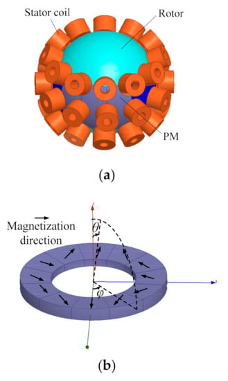
Figure 1.
The finite element method (FEM) model of the permanent magnet spherical motor (PMSM) has 12 permanent magnets and 36 stator coils and the magnetizing direction of Halbach array permanent magnet (PM). (a) FEM model of PMSM; (b) Magnetizing direction of Halbach array PM.

Table 1.
Parameters of the FEM of the PMSM.
Based on the FEM model shown in Figure 1a, adaptive mesh subdivision is employed. The boundaries between the PM, air gap, and winding meet the natural boundary condition. The outermost boundary region satisfies the first kind of homogeneous boundary conditions. Figure 2 shows the variation of radial component of the axial air-gap magnetic flux density () with θ, when = 0°, = 15°, and = 30°, respectively.
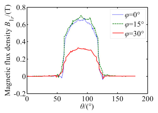
Figure 2.
The variation of radial component of the axial air-gap magnetic flux density () with θ, when = 0°, = 15°, and = 30°.
Figure 3 shows that has the same trend with θ under different paths, which is rapidly attenuated from the equator to the end of the PM, thus leading to the distortion of the main magnetic field inside the motor and the reduced the peak value of back-EMF [18]. Therefore, the axial air-gap magnetic field should be optimized to improve the performance of the motor. After the materials of the PM and iron core are determined, the main factors influencing the air-gap magnetic field of the motor are the structural parameters of the PM and the air-gap length of the motor. Therefore, in this paper, the thickness of PM (h), the latitude angle of PM (θ1), and the air-gap length (g) are selected as the optimization variables. The influence of the optimization variables on the fundamental harmonic amplitude and waveform distortion of the axial air-gap magnetic field is investigated.
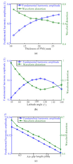
Figure 3.
The influence of each optimization variable on the amplitude and waveform of the axial air gap magnetic density. (a) The changing trend of the fundamental wave amplitude and waveform distortion rate of the axial air gap magnetic density with h; (b) the changing trend of the fundamental wave amplitude and waveform distortion rate of the air gap magnetic density with θ1; (c) the changing trend of the fundamental wave amplitude and waveform distortion rate of the air gap magnetic density with g.
In this paper, the waveform distortion of air-gap magnetic field is defined as the ratio of the root mean square of the higher harmonic amplitude to the fundamental harmonic amplitude.
where is the fundamental harmonic amplitude and is the higher harmonic amplitude. The harmonics amplitudes are obtained by Fourier transform.
Keeping the other parameters unchanged, h is changed from 11.1 mm to 25.1 mm. Figure 3a shows the changing trend of the fundamental wave amplitude and waveform distortion rate of the axial air gap magnetic density with h. It is shown that the fundamental harmonic amplitude increases with the increase of h, but the increasing amplitude gradually gets smaller. The waveform distortion decreases with the increase of h. Considering the performance of the motor and the difficulty of magnet processing, h is selected within the range of 17.1–25.1 mm.
Keeping the other parameters unchanged, θ1 is changed from 40° to 160°. Figure 3b shows the changing trend of the fundamental wave amplitude and waveform distortion rate of the air gap magnetic density with θ1. In Figure 3b, with the increase of θ1, the fundamental harmonic amplitude first increases and then decreases, while the waveform distortion first decreases and then increases. Considering the performance of the motor and the fabrication difficulty of magnet, θ1 is selected within the range of 80°–120°.
Keeping the other parameters unchanged, g is changed from 0.2 mm to 2.0 mm. Figure 3c shows the changing trend of the fundamental wave amplitude and waveform distortion rate of the air gap magnetic density with g. Figure 3c shows that both the fundamental harmonic amplitude and waveform distortion decrease as g increases. Considering the performance of the motor, g is selected with the range of 0.4–1.6 mm.
The above harmonic analysis of the air gap magnetic field determines the reasonable selection range of design variables and lays a foundation for further optimization in the future.
3. Modeling of SVM and Calculation of Moment of Inertia
The main idea of SVM regression is to map the training sample to high-dimensional space through a nonlinear relationship. The key to establishing the SVM model is how to construct the relationship between input and output. In this paper, the radial basis function is chosen to construct the SVM model.
3.1. Support Vector Machine Regression Modeling Method
Let the training sample be , where is the number of training samples, is the input of the i-th sample, and is the output of the i-th sample. The sample space is mapped to a high-dimensional feature space through the nonlinear function (), and then linear regression is performed. The regression function is
where is the weight and b is the offset.
It is assumed that the linear regression function can accurately fit the sample space data under the accuracy . Then,
Then, the regression problem can be reduced to the following optimal one.
Then, the following formula can be obtained:
where is a term related to the complexity of the function f, ε is the insensitive loss function, , is the relaxation factor, and C is the penalty factor.
Lagrange multipliers are used to solve the convex quadratic naturalization problem, the results are shown as follows:
and the constraint conditions are satisfied.
where , represents the Lagrange multiplier. Then, the available weight w is
SV stands for support vector. Then, the regression function of the support vector machine can be expressed as
For nonlinear regression problems, the sample space can be transformed into a high-dimensional space through nonlinear transformation, and linear regression analysis can be performed in the high-dimensional space. In a high-dimensional space, the kernel function K( is used to replace the dot product ( in the above formula, so that
3.2. The Choice of Kernel Function and the Influence of its Parameters on Regression
The form of the kernel function and the value of its parameters affect the complexity and accuracy of the SVM regression model. SVM nonlinear regression modeling is to map a nonlinear sample space to a high-dimensional space through a kernel function, and then perform linear regression. Only with an appropriate choice of kernel function type and corresponding kernel parameters can an SVM regression model with good generalization ability be constructed. This paper chooses the RBF kernel function to construct the SVM regression model, and its expression is
The kernel function parameter and penalty factor C in the SVM model have an important impact on the establishment of an accurate SVM model. The penalty factor C is used to measure the tolerance to training errors, and the kernel function parameter determines the distribution of the sample space mapped to the high-dimensional space. When is small, the training error is small. At this time, almost all of the sample data are support vectors, and the generalization ability of the SVM is poor. When gets larger, the support vector decreases, and the corresponding training error and test error increase. The generalization ability of the support vector machine is still relatively poor. When the value of the penalty factor C is smaller, the penalty for experience error is smaller. The less complex the learning machine, the greater the experience risk, and vice versa.
3.3. Establishment of Sample Space
Two sets of sample dots by FEM are built for the training and testing of SVM model. Table 2 shows the data distribution of the training sample space. From Table 2, sample dots need to be established. It is time consuming to build 125 models by FEM. Here, the Taguchi method based on orthogonal experiment is adopted [19]. The orthogonal experiment mainly relies on the number and level of the studied parameters. The advantage is that fewer experiments need to be conducted to obtain the best combination of design parameters.
Table 2.
The distribution of sample space.
According to Table 2, the orthogonal experiment L 25 () with three parameters and five levels is established. The corresponding parameter design and the finite element results of two objective functions are shown in Table 3. Twenty-five sample dots are used to build the SVM model, thus reducing the computational burden.
Table 3.
The orthogonal table and the results of FEM.
3.4. Parameter Optimization of SVM Model
The kernel function parameter σ and the penalty factor C in the SVM model have an important influence on the accuracy of SVM model [20]. The penalty factor C is used to measure the tolerance to training errors, and the kernel function parameter σ determines the distribution of sample space mapped to high dimensional space. In this paper, a GS algorithm is used to obtain the optimal SVM model parameters. The accuracy of the SVM regression model is measured by the root Mean Square Error (MSE), and its expression is as follows.
where and are the values from FEM and SVM, respectively.
Figure 4 shows the 3D diagram of the parameter optimization of the fundamental harmonic amplitude and waveform distortion of air-gap magnetic flux density. C and σ are within the range of (0,100), and the step is 0.1.
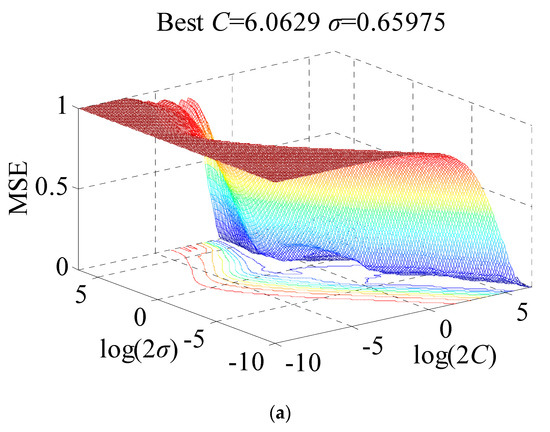
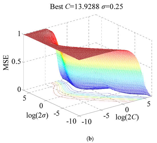
Figure 4.
The 3D diagram of the parameter optimization of the fundamental harmonic amplitude and waveform distortion of air-gap magnetic flux density. (a) Parameter optimization result of ; (b) parameter optimization result of the waveform distortion rate.
It can be seen from Figure 4 that, within a certain range, the MSE corresponding to C and σ is very small, while in most cases, the MSE is very large. Under normal circumstances, the optimal solution can be found using a large-scale and small-step grid, which, however, is often time-consuming. Therefore, an improved GS algorithm is proposed in this paper. First, the rough search is performed with large steps within a large range, and then the search space and step are gradually narrowed for detailed search. The detailed process is as follows:
- The initial search space is (0,100) and the initial step is 1. The rough search is performed to obtain an optimal parameter C and σ.
- Based on the obtained optimal parameter C and σ, the search space is halved, and a more accurate search is performed with a small step.
- Step 2 is repeated until the step size is reduced to 0.1, and with the search stopped, the optimal solution is then output.
In order to verify the effectiveness of the improved grid optimization algorithm, Table 4 and Table 5 show the comparison results of the optimization time and prediction error of the air gap magnetic density fundamental wave amplitude and waveform distortion rate obtained using the improved GS algorithm, the traditional GS algorithm, the PSO algorithm, and the genetic algorithm (GA), respectively.
Table 4.
The comparison among different algorithms for fundamental harmonic amplitude.
Table 5.
The comparison among different algorithms for waveform distortion.
According to Table 4 and Table 5, compared with traditional GS algorithms, the improved GS algorithm shows advantages including less optimization time and lower prediction error. Moreover, compared with the optimization results of PSO algorithm and GA algorithm, the improved GS algorithm is also better in optimization time and prediction error. The result shows that the improved GS algorithm improves the efficiency and accuracy of parameter optimization.
Based on the improve GS algorithm, the prediction errors of the fundamental harmonic amplitude and waveform distortion are 1.6382% and 1.3278%, respectively. This shows that the SVM model has good generalization capabilities. In addition, for the same sample data, much less time is used to calculate the output of SVM model than that of the FEM. Therefore, the SVM model can be used for the online calculation of parameter optimization of the PMSM [14].
3.5. Calculation of Moment of Inertia
PMSM is mostly applied in servo systems, which have a high requirement on the dynamic response and control accuracy of the motor. Therefore, in the optimization design of the PMSM, the moment of inertia of the rotor should be reduced. The expression of moment of inertia is
where is the moment of inertia of the rigid body, is the mass of the particle, and is the distance from the particle to the axis of rotation.
The rotor of the PMSM contains the PMs and the rotor yoke. According to (3), the expression of the moment of inertia of the PMSM can be obtained as
where is the moment of inertia with the z axis as the axis of rotation, is the outer radius of the PM, is the inner radius of the PM, is the mass density of the rotor yoke (= 1.02 g/cm3), and is the mass density of the PM (= 7.5 g/cm3).
4. Optimization and Verification
4.1. Optimization Theory
In this paper, there are three optimization goals, which belong to the multi-objective optimization problem. In multi-objective optimization, it is difficult to find a true optimal solution due to the conflicts between objectives. There are a series of solutions, which are characterized by the existence of at least one solution whose objective is superior to other objectives. Such solutions are called non-dominated solutions.
Based on the related mathematical model of the Halbach array permanent magnet spherical motor established in the previous chapter, the linear weighted summation method is used to transform the multi-objective optimization problem into a single-objective one. By assigning different weights to different objective functions, a set of non-inferior solutions are obtained. The ordinal preference method that approximates the ideal solution is adopted to find the most satisfactory result from the non-inferior solutions, which was developed by Hwang and Yoon [21]. The basic theory is based on the smallest difference between the selected plan and the ideal plan, and the largest difference between the selected plan and the negative ideal plan.
Supposing that there are n attributes and m solutions in an optimization problem, which correspond to a geometric system of m points in a n-dimensional space, the coordinates of each point are determined by the standardized weighted attribute values of each solution. Within comparison with the positive ideal solution and the negative ideal solution, the advantages and disadvantages of each scheme are judged. The specific process is as follows:
- The normalized decision matrix is obtained by normalization method. Suppose that the decision matrix of the multi-attribute decision-making problem is , and the standardized decision matrix is , then
- Construct a weighted normalization matrix. According to the weight coefficient given by the designer, multiply it by the standardized decision matrixwhere is the weight of the j-th objective function.
- Determine positive and negative ideal solutions.Positive ideal solution:Negative ideal solution:where is benefit type attribute, and is cost type attribute. is the j-th attribute value of positive ideal solution , and is the j-th attribute value of negative ideal solution .
- Calculate the distance from each scheme to the positive ideal and negative ideal solution under different weight coefficients. The distance from the objective function to the positive ideal solution is , and the distance to the negative ideal solution is .
- Calculate the closeness of the solution.where 0 When = 0, it means that the scheme is the worst scheme; when = 1, it means that the scheme is the best one.
- Sort the according to the calculated size of . The larger the , the better the solution.
Figure 5 shows the basic flow chart of the technique.
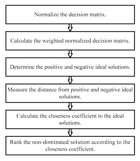
Figure 5.
Flow chart of ordinal preference method which approximates the ideal solution.
4.2. Multi Objective Optimization of PMSM
For the multi-objective optimization of the PMSM, the weight coefficient method is employed to transform multi-objective optimization into single objective optimization. In this paper, the aim of optimization is to obtain the relatively maximum fundamental harmonic amplitude, and the relatively minimum waveform distortion and the moment of inertia. So, the fitness function F can be designed as:
where and are the reference values of fundamental wave amplitude and waveform distortion rate, respectively. When h = 19.1 mm, = 60°, and g = 1 mm, and are 0.3170 T, 0.6519, respectively. , , and are the weights corresponding to the fundamental wave amplitude, waveform distortion rate, and moment of inertia. represents the function of fundamental harmonic amplitude and represents the function of waveform distortion, both of which are the functions of h, g, . is the normalized expression of moment of inertia, and as the function of h, , it can be expressed as
where is the moment of inertia when h = 17.1mm and = 80°, is the moment of inertia when h = 25.1 mm and = 120°, and is the moment of inertia with the z axis as the axis of rotation.
From the above analysis, the multi-objective optimization problem in this paper can be expressed as
In the optimization design of this article, the population number of the particle swarm algorithm is set as 50, the number of iterations as 1000, and the learning factor as 1.4944. Different weighting coefficient ratios will produce different optimization results, and each weighting ratio is determined according to the researcher’s preference or engineering needs. In this paper, 36 sets of weighting ratios are randomly generated in the form of grid division, the sum of weight coefficients is 1, and 36 sets of weighting ratios are generated in the interval 0–1 with a step of 0.1, that is, 36 optimization schemes. Table 6 shows the optimization results obtained by using the particle swarm algorithm under different weight coefficients (the optimization results are the normalized ones). Figure 6 is a three-dimensional graph drawn based on the optimization results in Table 6.
Table 6.
Optimization results under different weight coefficients.
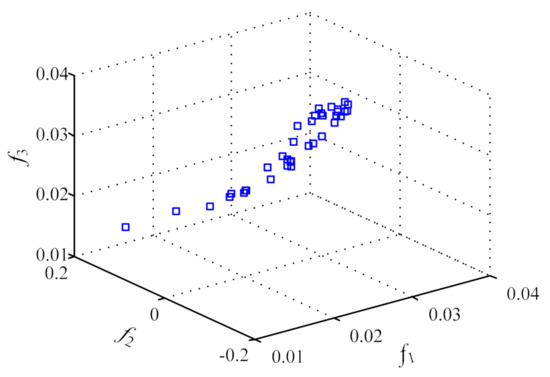
Figure 6.
Distribution of the non-dominated solutions.
Figure 6 shows the distribution of solutions using PSO with different weight coefficients. Each point represents a feasible solution.
However, it is difficult to find the optimal solution directly from it. The mathematical evaluation of the non-dominated solutions is implemented based on the ordinal preference method which approximates the ideal solution. Figure 6 shows the basic flow chart of the technique. According to the distribution of feasible solutions in Figure 6 and the evaluation method in Figure 5, Figure 7 gives the evaluation results of the feasible solutions.
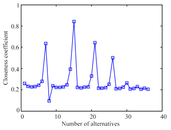
Figure 7.
Evaluation results of the feasible solutions.
It can be seen from Figure 7 that the 15th group of feasible solutions has the largest closeness coefficient. Therefore, this solution is the best one. According to the evaluation results, the corresponding optimization result is h = 23.3484 mm, θ1 = 113.46°, and g = 0.8951 mm. Considering the fabrication of the PM, h = 23.3 mm, θ1 = 113°, and g = 0.9 mm are selected.
4.3. Verification
The structural parameters of the Halbach array permanent magnet spherical motor before and after optimization are shown in Table 7.
Table 7.
Structure parameters of non-optimized and optimized motor.
Figure 8 shows the comparison of non-optimized and optimized axial air-gap flux density when = 0°.
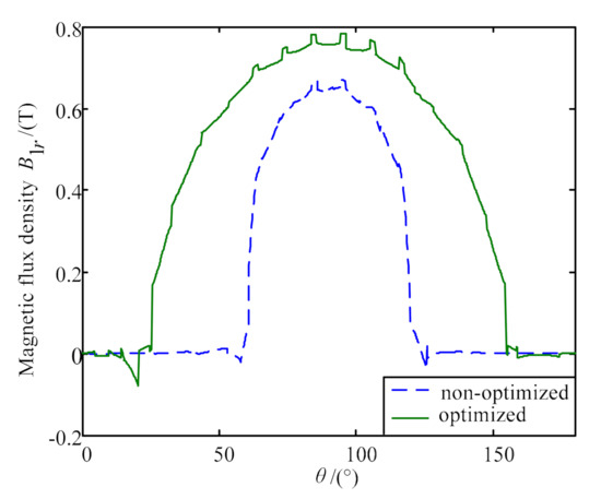
Figure 8.
The comparison of non-optimized and optimized axial air-gap flux density.
From Table 7 and Figure 8, the waveform distortion is obviously reduced, and the fundamental harmonic amplitude is greatly improved for the optimized PMSM.
Under no-load conditions, the rotation speed is 30 rpm. Figure 9a shows the comparison of the influence on the back EMF of the permanent magnet spherical motor with and without the end effect considered before the optimization. Figure 9b shows the comparison of the influence on the back EMF of the permanent magnet spherical motor with and without the end effect considered after the optimization.
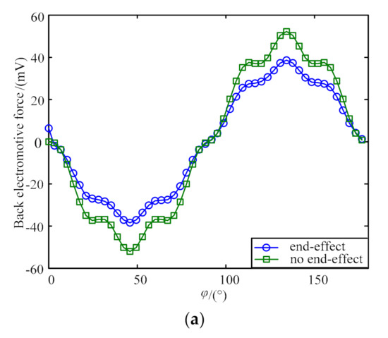
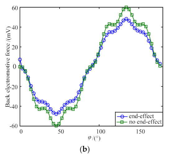
Figure 9.
Comparison of non-optimized and optimized spinning back EMF. (a) The comparison of the influence on the back EMF of the permanent magnet spherical motor with and without the end effect considered before the optimization; (b) the comparison of the influence on the back EMF of the permanent magnet spherical motor with and without the end effect considered after the optimization.
It is shown in Figure 9 that the peak value of the spinning back-EMF with the end effect considered is significantly smaller than that without the end effect considered, and the optimized PMSM has a smaller difference between the peak values with and without the end effect considered. Here, a coefficient S is defined to measure the influence of the end effect on the spinning back-EMF.
where is the peak value of the spinning back-EMF without the end effect considered and is the peak value of the spinning back-EMF with the end effect considered. The smaller the ratio, the smaller effect of the end effect on the spinning back-EMF. The coefficients corresponding to Figure 9a,b are 0.3499 and 0.2449, respectively. It can be obtained that the end effect has an influence on the peak value of the spinning back-EMF. For the optimized PMSM, the influence of the end effect on the spinning back-EMF is weakened.
Figure 10 shows the variation of the spinning torque and tilting torque generated by a single coil. From Figure 10a, the optimized spinning torque has a larger peak value. The Fourier decomposition of the torque is carried out. Before the optimization, the fundamental amplitude and waveform distortion rate of the rotation torque are 113.6380 mT and 0.0989, respectively. After the optimization, the fundamental wave amplitude and waveform distortion rate of the rotation torque are 143.7316 mT and 0.0950, respectively.
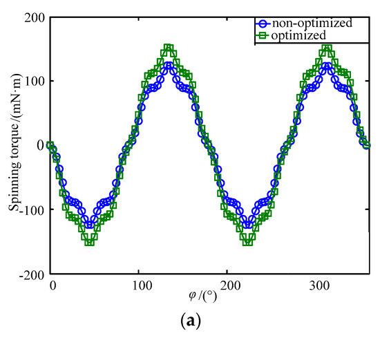
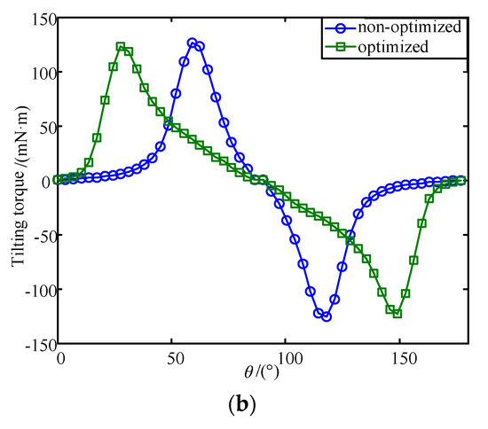
Figure 10.
Torque comparison of PMSM before and after optimization. (a) Comparison of the spinning torque of PMSM before and after optimization; (b) comparison of the tilting torque of PMSM before and after optimization.
The Fourier decomposition of the torque is carried out. Before the optimization, the fundamental amplitude and waveform distortion rate of the tilting torque are 54.6160 mT and 0.9851 respectively. After the optimization, the fundamental wave amplitude and waveform distortion rate of the tilting torque are 73.1590 mT and 0.4810, respectively.
The result shows that the optimized torque characteristic is improved, which is helpful in improving the torque output and operation stability of the PMSM.
4.4. Verification by Experiment
A prototype shown in Figure 11 is manufactured. Figure 11a is the structure of Halbach array PM. Figure 11c is the assembled Halbach array PM of spherical motor rotor.
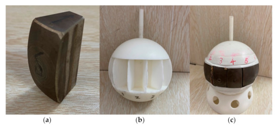
Figure 11.
Halbach array PM spherical motor: (a) the structure of Halbach array PM; (b) rotor yoke structure; (c) overall structure.
The experimental device for detecting the magnetic field is shown in the Figure 12.
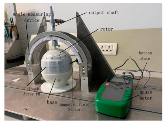
Figure 12.
The axial air-gap flux density measurement experimental platform of PMSM.
Figure 12 shows the optimized experimental device diagram, and the specific dimensions are given in Table 7. The variation of axial air gap flux density with latitude can be detected by making the output shaft yaw in the guide rail. The axial air gap magnetic field is detected by a fixed magnetic field sensor and its value is displayed in a Gauss meter. In this experiment, the reliability of the data needs to be ensured so as to reduce the error. The measurement is conducted every 5°, and three measurements are taken on the same track and the average value is used. The comparison between the experimental and analytical results of the optimized axial air gap flux density is shown in Figure 13.
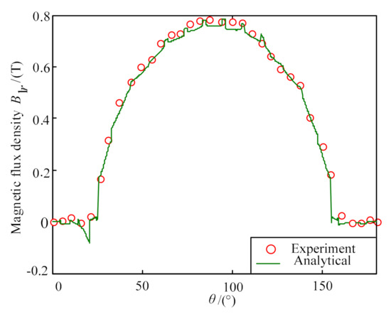
Figure 13.
The comparison of analytical solutions and experiment results.
It can be seen from Figure 13 that there is good agreement between the obtained axial air gap flux density model and the experiment results in waveform distribution and numerical values. The correctness of the magnetic field model established in this paper and the effectiveness of multi-objective optimization of axial air gap magnetic field are then verified.
5. Conclusions
In this paper, the axial air-gap magnetic field of the Halbach array PMSM is modeled based on SVM. The reasonable selection range of the design variables is determined through FEM. An improved GS algorithm is proposed to optimize the model parameter. At the same time, the influence of moment of inertia on the response speed of the motor is considered. Based on the established mathematical model, the optimal structure of the PMSM is obtained using PSO. The results show that the axial air-gap magnetic field of the optimized PMSM is improved. The influence of the end effect on the peak value of the back-EMF is weakened, and the performance of the electromagnetic torque is improved.
Author Contributions
Conceptualization, H.L. and B.L.; formal analysis L.C.; software and simulation, L.C. and Z.M.; writing—original draft, L.C.; writing—review and editing, L.C. All authors have read and agreed to the published version of the manuscript.
Funding
This work was supported by the National Natural Science Foundation of China under Grant 51877149 and 51677130 and the Research Programs funded by Tianjin Municipality under Grant 17JCTPJC46600.
Conflicts of Interest
The authors declare no conflict of interest.
References
- Wen, Y.; Li, G.; Wang, Q.; Tang, R.; Liu, Y.; Li, H. Investigation on the Measurement Method for Output Torque of a Spherical Motor. Appl. Sci. 2020, 10, 2510. [Google Scholar] [CrossRef]
- Zhu, L.; Guo, J.; Gill, E. Review of Reaction Spheres for Spacecraft Attitude Control. Prog. Aerosp. Sci. 2017, 91, 67–86. [Google Scholar] [CrossRef]
- Xia, C.; Li, H.; Shi, T. 3-D Magnetic Field and Torque Analysis of a Novel Halbach Array Permanent-Magnet Spherical Motor. IEEE Trans. Magn. 2008, 44, 2016–2020. [Google Scholar]
- Li, H.; Li, T. End-Effect Magnetic Field Analysis of the Halbach Array Permanent Magnet Spherical Motor. IEEE Trans. Magn. 2018, 54, 1–9. [Google Scholar] [CrossRef]
- Rossini, L.; Mingard, S.; Boletis, A. Rotor Design Optimization for a Reaction Sphere Actuator. IEEE Trans. Ind. Appl. 2014, 50, 1706–1716. [Google Scholar] [CrossRef]
- Liang, Y.; Delong, L.; Zongxia, J. Magnetic field modeling based on geometrical equivalence principle for spherical actuator with cylindrical shaped magnet poles. Aerosp. Sci. Technol. 2016, 49, 17–25. [Google Scholar]
- Bin, L.; Zhitian, L.; Guidan, L. Magnetic Field Model for Permanent Magnet Spherical Motor with Double Polyhedron Structure. IEEE Trans. Magn. 2017, 53, 2016–2020. [Google Scholar]
- Bin, L.; Chao, L.; Li, H. Torque analysis of spherical permanent magnetic motor with magnetic equivalent circuit and Maxwell stress tensor. In Informatics in Control, Automation and Robotics; Springer: Berlin/Heidelberg, Germany, 2011; Volume 133, pp. 617–628. [Google Scholar]
- Nakamura, H.; Mizuno, Y. Method for Diagnosing a Short-Circuit Fault in the Stator Winding of a Motor Based on Parameter Identification of Features and a Support Vector Machine. Energies 2020, 13, 2272. [Google Scholar] [CrossRef]
- Niu, D.; Dai, S. A Short-Term Load Forecasting Model with a Modified Particle Swarm Optimization Algorithm and Least Squares Support Vector Machine Based on the Denoising Method of Empirical Mode Decomposition and Grey Relational Analysis. Energies 2017, 10, 408. [Google Scholar] [CrossRef]
- Bao, X.H.; Wang, Q.J.; Ni, Y.Y.; Qian, Z. Modeling and Parameters Optimal Design of Claw-Pole Alternator. Proc. CSEE 2006, 26, 138–142. [Google Scholar]
- Bao, Y.; Wang, X.; Ni, Q.; Jiang, W. Electromagnetic Modeling and Parameter Optimization of Claw-Pole Alternator for Automobile Application. Trans. China Electrotech. Soc. 2008, 23, 23–27. [Google Scholar]
- Ju, L.; Wang, Q.; Qian, Z. Modeling and optimization of spherical motor based on support vector machine and chaos. In Proceedings of the International Conference on Electrical Machines & Systems, Tokyo, Japan, 15–18 November 2009; pp. 1–4. [Google Scholar]
- Li, Z.; Zhang, L.; Lun, Q.; Jin, H. Optimal Design of Multi-DOF Deflection Type PM Motor by Response Surface Methodology. J. Electr. Eng. Technol. 2015, 10, 965–970. [Google Scholar] [CrossRef]
- Sakthivel, V.P.; Bhuvaneswari, R.; Subramanian, S. Multi-objective parameter estimation of induction motor using particle swarm optimization. Eng. Appl. Artif. Intell. 2010, 23, 302–312. [Google Scholar] [CrossRef]
- Jianjian, F.; Jianhua, W.; Lei, S. Multi-Objective Particle Swarm optimization of Alnico in Permanent Magnet Synchronous Motor. Trans. China Electrotech. Soc. 2009, 24, 53–58. [Google Scholar]
- Xia, C.; Xin, J.; Li, H. Design and analysis of a variable arc permanent magnet array for spherical motor. IEEE Trans. Magn. 2013, 49, 1470–1478. [Google Scholar] [CrossRef]
- Shi, T.; Song, P.; Li, H. End-effect of the permanent magnet spherical motor and its influence on back-EMF characteristics. Sci. China Technol. Sci. 2012, 55, 206–212. [Google Scholar] [CrossRef]
- Zhang, B.; Wang, A.; Doppelbauer, M. Multi-objective optimization of a transverse flux machine with claw-pole and flux-concentrating structure. IEEE Trans. Magn. 2016, 52, 1–10. [Google Scholar] [CrossRef]
- Ju, L.; Wang, Q.; Li, G. Parameter Optimization for Support Vector Machine Model of Permanent Magnet Spherical Motors. Trans. China Electrotech. Soc. 2014, 29, 85–90. [Google Scholar]
- Hwang, C.L.; Yoon, K. Multiple Attribute Decision Making—Methods and Applications: A State-of-Art Survey; Springer: New York, NY, USA, 1981. [Google Scholar]


Publisher’s Note: MDPI stays neutral with regard to jurisdictional claims in published maps and institutional affiliations. |
© 2020 by the authors. Licensee MDPI, Basel, Switzerland. This article is an open access article distributed under the terms and conditions of the Creative Commons Attribution (CC BY) license (http://creativecommons.org/licenses/by/4.0/).