Abstract
Biomass gasification is the most reliable thermochemical conversion technology for the conversion of biomass into gaseous fuels such as H2, CO, and CH4. The performance of a gasification process can be estimated using thermodynamic equilibrium models. This type of model generally assumes the system reaches equilibrium, while in reality the system may only approach equilibrium leading to some errors between experimental and model results. In this study non-stoichiometric equilibrium models are modified and improved with correction factors inserted into the design equations so that when the Gibbs free energy is minimized model predictions will more closely match experimental values. The equilibrium models are implemented in MatLab and optimized based on experimental values from the literature using the optimization toolbox. The modified non-stoichiometric models are shown to be more accurate than unmodified models based on the calculated root mean square error values. These models can be applied for various types of solid biomass for the production of syngas through biomass gasification processes such as wood, agricultural, and crop residues.
1. Introduction
In recent decades alternative sustainable energy sources have been being considered and utilized to decrease dependency on fossil fuels. Biomass is one of the most favorable and promising clean energy sources which is neutral in terms of carbon dioxide (CO2) and emits lower amounts of greenhouse gases [1,2]. Biomass can be used in direct combustion to generate energy in the form of heat or can be transformed into more valuable gaseous and liquid fuels, for example generating vehicle fuel, providing the heating for industrial unit operations, and generating heat and electricity for household use [3,4].
Different technologies have been developed to convert solid biomass into renewable fuels such as thermochemical, biological, and mechanical conversion methods. Thermochemical conversion technologies can be categorized as gasification, pyrolysis, combustion, and liquefaction [5,6,7,8,9,10]. Among these technologies, biomass gasification is considered as a reliable conversion technology due to the production of clean syngas for the efficient generation of heat and power while leading to relatively low emissions of pollutant [11,12]. Biomass gasification is a thermochemical conversion process which converts solid biomass feedstock into a mixture of gaseous components including hydrogen (H2), carbon monoxide (CO), carbon dioxide (CO2), and methane (CH4) through partial oxidization [13,14]. In addition to these major products, some minor products such as a nitric oxide (NO), nitrogen dioxide (NO2), water vapors (H2O), ammonia (NH3), hydrogen cyanide (HCN), hydrogen sulphide (H2S), sulphur dioxide (SO2), and sulphur trioxide (SO3) may also be observed as well as some amount of tar and char [15,16,17]. The composition of these major and minor products and the quality of the syngas from gasification depends on the biomass type, gasification agent, gasifier type, and operating parameters [18,19]. After cleaning or removing the undesirable compounds from syngas, it can be employed as a fuel in gas fired engines and turbines [20]. Biomass gasification is also favorable compared to combustion because it leads to lower emissions of SOx and NOx in the environment [21]. Dioxins and furans may also be observed which can be reduced by using hydro-gasification processes [22].
Various studies have looked at the modeling and simulation of biomass gasification processes which can generally grouped into three different kinds of models: (a) kinetic models, (b) computational fluid dynamic models, and (c) thermodynamic equilibrium models [17,23,24]. Kinetic models [25] are quite complex models because they depend on the reaction mechanism of various chemical reactions occurring in the gasifier. These kinds of models are suitable for the prediction of process parameters and gasifier design. Computational fluid dynamics models [26] are also very complex models because a wide variety of physical phenomena (such as particle geometry and fluid flow properties etc.) are required for the simulation and they also included sub-models related to the oxidation, vaporization, and pyrolysis. Thermodynamic equilibrium models [16,27,28] are simple and can be solved using less computation time than more complex kinetic and CFD models. While dealing with experiments, equilibrium conditions may not be achieved in the gasifier but these thermodynamic models give an estimation of the output composition of the syngas. There are two approaches to equilibrium modelling: (a) stoichiometric and (b) non-stoichiometric models. Stoichiometric models [27,29] are developed on the assumption that certain chemical reactions reach equilibrium and solving this type of model requires calculation of the associated equilibrium constants. For the non-stoichiometric models [16,17,30] the equilibrium is determined by minimizing the Gibbs free energy of the reaction products without specifying any given reactions in the gasification process.
In the previous studies many researchers have developed non-stoichiometric equilibrium models based on proposed global gasification reactions which specify the major and minor products [16,30,31]. For the first time, Altafini et al. [31] developed a modified equilibrium model based on the minimization of Gibbs free energy. They considered the five components of biomass feedstock such as carbon (C), hydrogen (H), oxygen (O), nitrogen (N), and sulphur (S). They modified the model by considering a heat loss of 1% in the energy balance and optimized using the Lagrange multipliers method. Jarungthammachote and Dutta [30] modified the model proposed by Altafini et al. [31] for the different bed gasifiers. Their model is modified by considering the effect of the carbon conversion on the major components of the syngas such as H2, CO, CO2, CH4, and N2. Buragohain et al. [32] developed a semi-equilibrium model by minimizing the Gibbs free energy. They considered four different carbon conversion levels i.e., 70%, 80%, 90%, and 100%, and compared the results at each level. Kangas et al. [33] developed an equilibrium model (minimizing Gibbs free energy) considering some hydrocarbon species as a minor product in the gaseous phase, water vapors in the liquid phase and SiO2 is considered in solid-phase with unreacted carbon. Gambarotta et al. [16] developed a non-stoichiometric equilibrium model considering 16 products and used the carbon conversion factor (unreacted carbon) proposed by Azzone et al. [27]. Based on these previous studies it is clear that three types of modifications have been considered in non-stoichiometric models including: carbon conversion efficiency, gasification efficiency, and the amount of heat loss in energy balance.
In this study non-stoichiometric thermodynamic equilibrium models have been formulated with and without the carbon conversion factor to predict the syngas composition from the biomass gasification process. These models are further modified by adding correction factors in the Gibbs energy equations which are solved for each component of the syngas (in this case Equations (6)–(10)). These correction factors are generated by optimizing the formulated models using a large data set of biomass gasification experiments in the MatLab optimization toolbox. These models are validated with experimental values from the literature and compared to show any improvement in model accuracy resulting from the correction factors.
2. The Non-Stoichiometric Thermodynamic Equilibrium Model
To develop the non-stoichiometric equilibrium models, the following assumptions have been considered.
- The biomass feedstock consists of carbon, hydrogen, oxygen, and nitrogen.
- N2 is considered to be inert.
- Alkalies and metal contents in the biomass are neglected.
- Ash is considered as inert.
- The syngas consists of H2, CO, CO2, CH4, and N2 [34].
- Minor products compounds containing sulphur and nitrogen (e.g., SOx and NOx are neglected).
- Downdraft gasifier produces a very low amount of tar [27,35] which is neglected in this model.
- The biomass feedstock and the air enters into the gasifier at the temperature of 25 °C and the gasifier pressure is 101.13 kPa.
- Heat losses are not considered and the system is considered as adiabatic.
The global gasification reaction inside the gasifier is considered as follow:
where is the molecular formula of biomass and is the amount of the water moisture in the solid biomass feed (per mole of carbon in the biomass). The Nitrogen to oxygen molar ratio is denoted by (e.g., 3.76 for the standard air) and m is the moles of the oxygen in the air entering into the gasifier. Azzone et al. [27] introduced an factor for the carbon conversion efficiency. The subscripts are derived from the given ultimate analysis of biomass. The terms of are the moles of and unreacted carbon, respectively, in the product per mole of carbon in the feed.
To predict the syngas composition, the mass balance constraints are as follow:
Carbon balance:
Hydrogen Balance:
Oxygen Balance:
To solve this equlibrium system, the Lagrange multiplier method is applied and is introduced for every element as , and . There are three Lagrange multipliers because there are three main elements considered in this model. The Lagrangian function which shows the total Gibbs free energy of the gas mixture composed by M components at equilibrium conditions is given as:
where and are the standard Gibbs free energy and moles of the i-th species, R is the ideal gas constant, and . The function can be minimized when all the partial derivatives of the Lagrangian function are equal to zero. The partial derivatives of the Lagrangian function can be written as follow:
where (kJ/mol) is the standard Gibbs function of formation which is the function of temperature T of the every gas species. This function can be expressed as follow:
The constant values of () and enthalpy of formation are given in Table 1 [36].

Table 1.
The values of (kJ/mol) and the coefficients of Equation (11) (kJ/mol).
All the Equations (2)–(11) are solved by the Newton–Raphson iterative method to find the values of the unknowns ,.
Energy Balance
The reaction temperature of the gasifier is the temperature that fulfills the energy balance Equation (12). This equation can also be helpful to calculate the amount of the entering air or oxygen used for the oxidation reactions.
where which can be calculated as follow [37]:
where lower heating value (LHV) of the biomass is the function of higher heating value (HHV) of the biomass that can be calculated as following [38]:
where the specific heat Cp (kJ/kmol K) in Equation (12) at constant pressure is a function of the gasification temperature which can be calculated as follow:
where T is the gasification temperature in K and
where z is the integral constant and the coefficients(A’–D’) of specific heat are given in Table 2 [39].
HHV = 0.3491 C + 1.1783 H + 0.1005 S − 0.1034 O − 0.0151 N − 0.0211 Ash
Table 2.
The coefficients of specific heat (kJ/mol) in Equation (17).
3. Model Implementation
There are a total of eight unknown defined in the non-stoichiometric equilibrium model which are representing the syngas composition , unreacted carbon , and Lagrange multipliers . Therefore, eight equations are needed to find the unknowns. These eight equations are; three mass balance equations (Equations (2)–(4)) and five equations for the Lagrangian function (Equations (6)–(10)). These equations are solved by the Newton–Raphson method in MATLAB as shown in Figure 1. Four non-stoichiometric thermodynamic equilibrium models have been developed to estimate the syngas composition from the biomass gasification process. The details of all these models have been shown in Table 3.
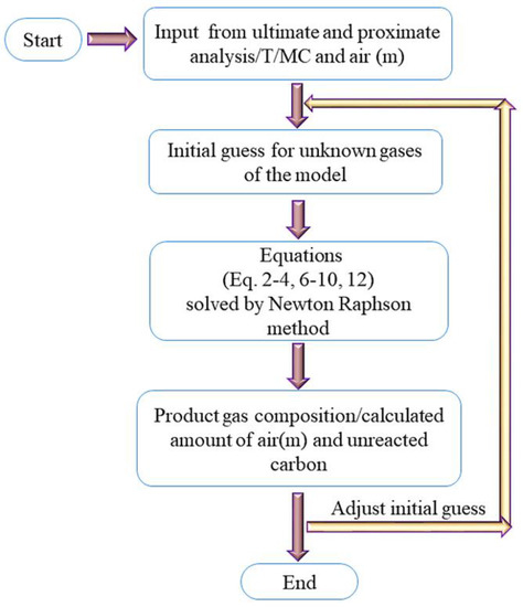
Figure 1.
Model algorithm.
Table 3.
The details of the models.
4. Results and Discussion
The accuracy of the developed models and modified models had been trained and optimized by the large data set of 32 experiments. These models are also tested by the 18 experiments and validated with the already published modeling studies. The data from these experiments for training and testing is listed in the Supplementary Materials. The biomass feedstock data used for the training and the testing is shown in Table 4 including many of the same biomass types considered by Aydin et al. [34]. The effect of ash is not expected to have a significant affect on the models, with relatively small ash content and a minor effect through Equation (15). Finally, the root mean square error (RMSE) is calculated for comparisons and to check the accuracy of the developed models as in Equation (18).
Table 4.
Ultimate and proximate analysis of different biomass feedstocks. (% dry mass for composition and MJ /kg of dry mass for HHV and LHV).
4.1. Model Modification
Model M1 is the general non-stoichiometric equilibrium model which is based on a global gasification reaction. This model predicts the syngas composition considering the complete carbon conversion without any modification. Model M2 is an extension of model M1 considering the unreacted carbon with the syngas composition at the end of the gasification process. Model M3 and Model M4 are the modified versions models M1 and M2, respectively. These models are modified by introducing correction factors in each Gibbs equation for each component of the syngas.
These correction factors are found by optimizing the formulated non-stoichiometric models using data from published experimental studies. These models are implemented in MatLab and “fminumc”, a built-in optimization function in MatLab, is used to optimize the correction factors so that the predicted composition of syngas more closely matches with experimental values. This involved minimizing the root mean square error (RMSE) with respect to experimental results (32 sets of experimental data). After optimization the fitted correction factors are shown in Table 5.
Table 5.
Correction factors for the Models M3 and M4.
These correction factors are used in each Gibbs equation for each component of the gas from Equations (6)–(10) given as the modified Equation (19).
4.2. Model Validation
The developed models in this study had been validated against the published experimental [48], stoichiometric [27] and non-stoichiometric [16] modeling studies in the literature. These models presented the major product of the biomass gasification process such as H2, CO, CO2, CH4, and N2. Therefore, the model validation is also considered against these major products. Validation is done by taking wood biomass (a = 1.44, b = 0.66, and moisture content (MC) = 20%) at a temperature (T) of 1073 K. It can be seen that the literature models overestimates the volume or mole fraction of hydrogen and underestimate the fraction of carbon monoxide, carbon dioxide, and methane. The two developed models M1 and M2 show a similar behaviour with RMSE values similar to the two models form the literature. The RMSE of M1 and M2 are 1.9966 and 1.9034 while the RMSE of the non-stoichiometric and stoichiometric in the literature are 2.1887 and 1.8910. Moreover, 94% carbon conversion (α) is achieved in models M2 and M4 at the conditions mentioned in Table 6.
Table 6.
Non-stoichiometric models validations in volume fractions (%) at T = 1073 K and MC = 20%.
The modified models M3 and M4 are also compared with the experimental and modeling results. Table 6 shows a comparison between the modified developed model with other experimental and modeling results. The fraction of hydrogen is almost identical or similar to the experimental hydrogen fraction. While carbon monoxide and carbon dioxide are underestimated, and methane is overestimated. Although there is still room for improvement the modified models are shown to have improved accuracy compared to existing published models.
4.3. Comparison of Objective Function
The comparison of the overall root mean square error of all the developed and modified models using the 32 experimental training set data is shown in Table 7. This training set is used in the optimization to estimate values of Cr1 and Cr2. Model M1 showed the highest value 2.25 of the overall RMSE while the value for model M2 is 1.8676. Model M2 is possibly more accurate because it considers and estimates the amount of carbon converted while model M1 considers complete conversion. The overall RMSE of model M3 and M4 is 1.49 and 1.23, respectively, which are clearly lower than the equivalent models without correction factors (M1 and M2). Among all these non-stoichiometric thermodynamic equilibrium models, Model M4 showed the lowest overall RMSE. This model can be used for any type of solid biomass to estimate the syngas composition from the biomass gasification process. The Individual root mean square of each case in training is showed in Figure 2. The comparison of the testing data set of 18 experiments is shown in Table 8. This testing data have not been used in the optimisation, in this way it gives a fair comparison of the different models. The testing data set also showed the same trend as the training data set showed.
Table 7.
The overall room mean square error (RMSE) of all four models based on the training data set.
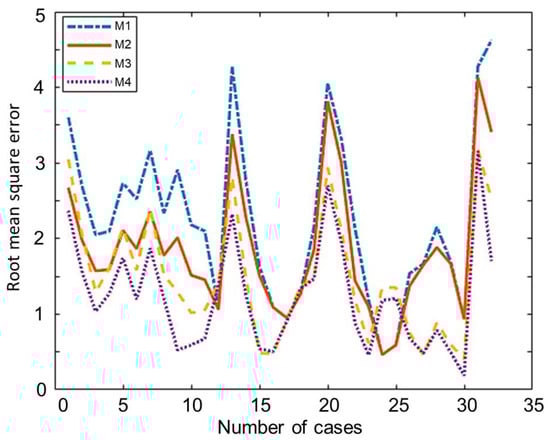
Figure 2.
Individual root mean square error (RMSE) of each case in training.
Table 8.
The overall RMSE of all four models based on testing data set.
4.4. Comparison of the Syngas Composition
The composition of the major species of syngas obtained from all non-stoichiometric models and experimental studies can be observed in Figure 3, Figure 4, Figure 5, Figure 6 and Figure 7. Figure 3 shows the composition of hydrogen gas from all models and experiments, and this shows that models M1 and M2 overestimate the composition while models M3 and M4 gave a very close estimation of hydrogen gas. Figure 4 shows a comparsion of models and experiment for carbon monoxide. This shows that all the models except model M4 overestimate the composion of CO gas for most of the experiments and Model M4 gave the closest values of composition with respect to the experiments. Figure 5 shows that all the models underestimate the prediction of carbon dioxide, but still model M4 gives the best estimation of carbon dioxide for these experiments. Figure 6 shows the model and experimental value of methane composition. In the thermodynamic equilibrium models, we observed that the methane gas was under-predicted for the models without modification and overestimated for models with the added correction factors. The composition of methane gas is not as important as the other gases in the syngas. Figure 7 shows the composition of nitrogen gas as predicted by the models and the experimental values. Nitrogen gas represents a large fraction of the product gas because it enters in large quantities through the air fed into the gasifier. Models M1, M2, and M3 are shown to underestimate this nitrogen fraction for most of the biomass cases while model M4 gave the best estimation for most these experiments.
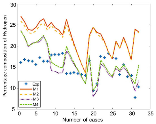
Figure 3.
Comparison of hydrogen composition given by experiments and models.
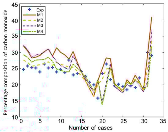
Figure 4.
Comparison of carbon monoxide composition given by experiments and models.
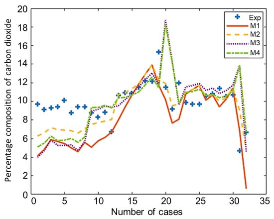
Figure 5.
Comparison of carbon dioxide composition given by experiments and models.
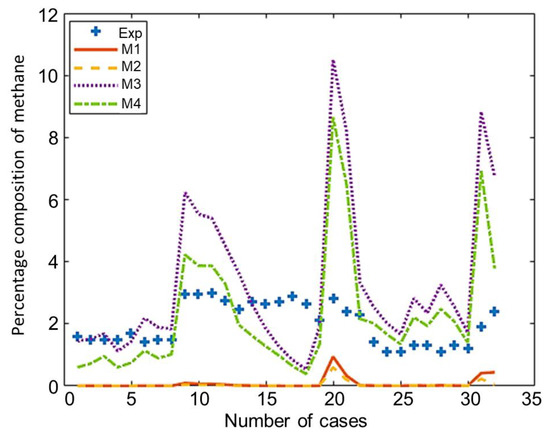
Figure 6.
Comparison of methane composition given by experiments and models.
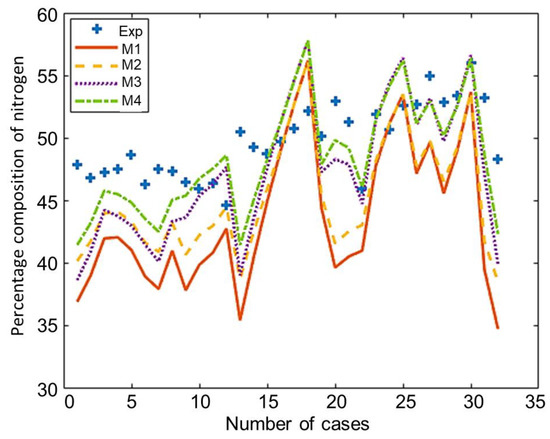
Figure 7.
Comparison of nitrogen composition given by experiments and models.
4.5. Effect of Parameters on Syngas Composition
The main parameters in this study that influence the composition of syngas are the moisture content of the biomass, the temperature of the gasification process, and the equivalence ratio (ER). This is investigated here for the validation case given in Table 6.
4.5.1. Effect of Biomass Moisture Content
Figure 8 shows the effect of the moisture content of woody biomass on the composition of syngas at 1073 K. Figure 8a–d show the effect on syngas composition as predicted by the models M1, M2, M3, and M4, respectively. From these figures it can be seen that there is a very small decrease in the composition of inert nitrogen (N2) as a result of increasing the moisture content. It is also observed that the composition of the H2 and CO2 increase and the composition of CO is decreases with increasing moisture content. Although CH4 is produced in very small quantities in air gasification, the trend shows that the composition of CH4 is decreases with increasing moisture content. From the figure, it can be seen that the highest quantities of H2 and CO can be achieved by increasing the moisture content as shown using modified models M3 and M4 (Figure 8c,d, respectively).
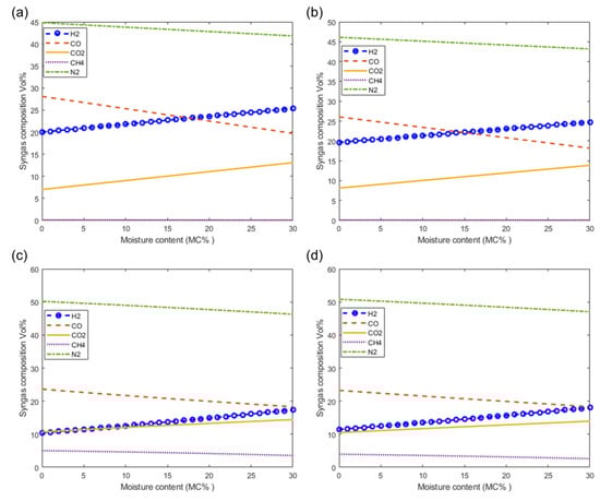
Figure 8.
Effect of moisture on syngas composition at T = 1073 K. As predicted by models (a) M1, (b) M2, (c) M3 and (d) M4.
4.5.2. Effect of Gasification Temperature
Figure 9 shows the effect of the gasification temperature on the syngas composition at the fixed moisture content of 20%. Figure 9a–d show the effect of gasification temperature on syngas composition as predicted by the models M1, M2, M3, and M4, respectively. From the figure, it is clearly observed that there is a decrease in the composition of inert nitrogen (N2) resulting from increasing the gasification temperature. It is also observed that the composition of the main components of syngas H2 and CO increase at higher gasification temperatures while the fraction of CO2 decreases at higher gasification temperatures. It is also observed the maximum fractions of H2 and CO can be obtained at temperatures of 1050 K and higher which also give the lowest fractions of CO2 and CH4 (Figure 9c,d).
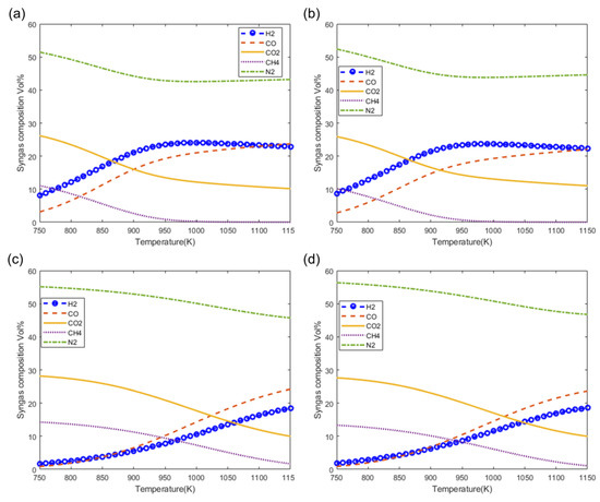
Figure 9.
Effect of gasification temperature on syngas composition at MC = 20%. (a) M1, (b) M2, (c) M3 and (d) M4.
4.5.3. Effect of Equivalence Ratio (ER)
Figure 10 shows the effect of the equivalence ratio on the syngas composition at a fixed moisture content of 20% and at a gasification temperature of 1073 K. Figure 10a–d show the effect of ER on syngas composition as predicted by the models M1, M2, M3, and M4, respectively. The composition of the N2 and CO2 increases with increasing ER values. It is also observed that the composition of the main components of the syngas H2 and CO decrease with increasing ER values.
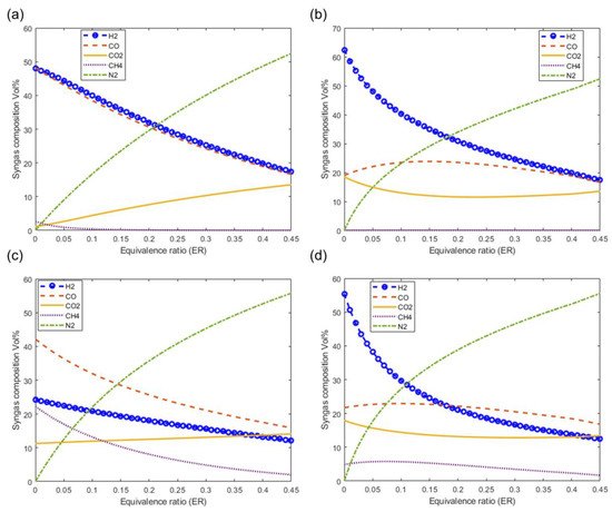
Figure 10.
Effect of equivalence ratio on syngas composition at T = 1073, MC = 20%. (a) M1, (b) M2, (c) M3 and (d) M4.
5. Conclusions
In this study, non-stoichiometric thermodynamic equilibrium models for the biomass gasification process have been formulated with and without considering the complete conversion of carbon to predict syngas composition. These models were modified by introducing correction factors in the Gibbs function for each component of syngas in the product. As far as we know this is the first study to consider correction factors added into Gibbs functions. These correction factors are obtained by optimizing the developed models based on 32 sets of experimental data using an optimization algorithm inside MatLab. Moreover, the modified models and the original models have been validated and compared against published experimental data and other modeling studies. The end results show that introducing correction factors in this way increases the model accuracy of the non-stoichiometric thermodynamic equilibrium models (with and without considering complete the carbon conversion). Model M4 which considers the estimation of carbon conversion (generally incomplete conversion) together with the added correction factors gave the lowest values of the overall RMSE for both training and testing experimental data. This model shows improved accuracy compared with thermodynamic equilibrium models which do not have correction factors. These modified models can be used to predict the syngas composition for any type of solid biomass feedstock at ranges of different operating conditions used inside gasification. Additionally, these models could potentially be improved by adding additional fitted parameters, which might allow a more accurate prediction and account for the influence of different operating and feed conditions.
Supplementary Materials
The following are available online at https://www.mdpi.com/1996-1073/13/21/5668/s1, Figure S1: Training Data, Figure S2: Testing Data.
Author Contributions
Conceptualization, H.M.U.A. and M.B.; methodology, H.M.U.A. and M.B.; validation, H.M.U.A.; data curation, H.M.U.A.; writing—original draft preparation, H.M.U.A.; writing—review and editing, M.B. and S.J.P.; supervision, M.B. All authors have read and agreed to the published version of the manuscript.
Funding
This research received no external funding.
Acknowledgments
Support is acknowledged from the SRD scholarship, Dongguk University, Seoul, South Korea.
Conflicts of Interest
The authors declared that there is no conflict of interest for this work.
Nomenclature
| C | Carbon mass fraction from the ultimate analysis |
| H | Hydrogen mass fraction from the ultimate analysis |
| O | Oxygen mass fraction from the ultimate analysis |
| N | Nitrogen mass fraction from the ultimate analysis |
| S | Sulphur mass fraction from the ultimate analysis |
| Ash | mass fraction of ash in biomass feedstock |
| Gfi | The standard Gibbs function of formation |
| a | number of hydrogen atoms per carbon atom in biomass molecule |
| b | number of oxygen atoms per carbon atoms in biomass molecule |
| c | Number of nitrogen atoms per carbon atoms in biomass molecule |
| w | the moisture of biomass (mole/mole of biomass) |
| m | moles of oxygen (mole/mole of biomass) |
| ρ | nitrogen to oxygen molar ratio in the oxidant |
| xi | coefficients of the product constituent |
| α | actual fraction of C participating in thermodynamic equilibrium reactions |
| specific heat capacity of component i | |
| The heat of formation of component i | |
| T | Gasification temperature |
| λi | Lagrangian multiplier |
| RMSE | Root mean square error |
| LHV | Lower heating value |
| HHV | Higher heating value |
| Cri | Correction factors |
| A’-D’ | Coefficients of specific heat |
| R | Ideal gas constant J/mol.K |
| ni | No. of moles of each component in Gibbs function |
| hfg | Heat of vaporization of water |
| Mi | Non-stoichiometricic model |
| z | integral constant |
| a’-g’ | Coefficients of the standard Gibbs function of formation |
References
- Mathieu, P.; Dubuisson, R. Performance analysis of a biomass gasifier. Energy Convers. Manag. 2002, 43, 1291–1299. [Google Scholar] [CrossRef]
- Ahmadi, P.; Dincer, I.; Rosen, M.A. Development and assessment of an integrated biomass-based multi-generation energy system. Energy 2013, 56, 155–166. [Google Scholar] [CrossRef]
- Sürmen, Y. The necessity of biomass energy for the Turkish economy. Energy Sources 2003, 25, 83–92. [Google Scholar] [CrossRef]
- Abdullah, A.; Ahmed, A.; Akhter, P.; Razzaq, A.; Zafar, M.; Hussain, M.; Shahzad, N.; Majeed, K.; Khurrum, S.; Bakar, M.S.A.; et al. Bioenergy potential and thermochemical characterization of lignocellulosic biomass residues available in Pakistan. Korean J. Chem. Eng. 2020, 37, 1899–1906. [Google Scholar] [CrossRef]
- Huda, A.; Mekhilef, S.; Ahsan, A. Biomass energy in Bangladesh: Current status and prospects. Renew. Sustain. Energy Rev. 2014, 30, 504–517. [Google Scholar] [CrossRef]
- Ong, H.C.; Chen, W.H.; Singh, Y.; Gan, Y.Y.; Chen, C.Y.; Show, P.L. A state-of-the-art review on thermochemical conversion of biomass for biofuel production: A TG-FTIR approach. Energy Convers. Manag. 2020, 209, 112634. [Google Scholar] [CrossRef]
- Uddin, M.; Techato, K.; Taweekun, J.; Rahman, M.M.; Rasul, M.; Mahlia, T.; Ashrafur, S. An overview of recent developments in biomass pyrolysis technologies. Energies 2018, 11, 3115. [Google Scholar] [CrossRef]
- Klemm, M.; Kröger, M.; Görsch, K.; Lange, R.; Hilpmann, G.; Lali, F.; Haase, S.; Krusche, M.; Ullrich, F.; Chen, Z. Experimental Evaluation of a New Approach for a Two-Stage Hydrothermal Biomass Liquefaction Process. Energies 2020, 13, 3692. [Google Scholar] [CrossRef]
- Qyyum, M.A.; Chaniago, Y.D.; Ali, W.; Saulat, H.; Lee, M. Membrane-Assisted Removal of Hydrogen and Nitrogen from Synthetic Natural Gas for Energy-Efficient Liquefaction. Energies 2020, 13, 5023. [Google Scholar] [CrossRef]
- Ahmed, A.; Abu Bakar, M.S.; Sukri, R.S.; Hussain, M.; Farooq, A.; Moogi, S.; Park, Y.K. Sawdust pyrolysis from the furniture industry in an auger pyrolysis reactor system for biochar and bio-oil production. Energy Convers. Manag. 2020, 226, 113502. [Google Scholar] [CrossRef]
- Hosseini, S.E.; Wahid, M.A.; Ganjehkaviri, A. An overview of renewable hydrogen production from thermochemical process of oil palm solid waste in Malaysia. Energy Convers. Manag. 2015, 94, 415–429. [Google Scholar] [CrossRef]
- Gadsbøll, R.Ø.; Thomsen, J.; Bang-Møller, C.; Ahrenfeldt, J.; Henriksen, U.B. Solid oxide fuel cells powered by biomass gasification for high efficiency power generation. Energy 2017, 131, 198–206. [Google Scholar] [CrossRef]
- Cau, G.; Tola, V.; Pettinau, A. A steady state model for predicting performance of small-scale up-draft coal gasifiers. Fuel 2015, 152, 3–12. [Google Scholar] [CrossRef]
- Farooq, A.; Song, H.; Park, Y.K.; Rhee, G.H. Effects of different Al2O3 support on HDPE gasification for enhanced hydrogen generation using Ni-based catalysts. Int. J. Hydrogen Energy 2020, in press. [Google Scholar] [CrossRef]
- Shayan, E.; Zare, V.; Mirzaee, I. Hydrogen production from biomass gasification; a theoretical comparison of using different gasification agents. Energy Convers. Manag. 2018, 159, 30–41. [Google Scholar] [CrossRef]
- Gambarotta, A.; Morini, M.; Zubani, A. A non-stoichiometric equilibrium model for the simulation of the biomass gasification process. Appl. Energy 2018, 227, 119–127. [Google Scholar] [CrossRef]
- Ferreira, S.; Monteiro, E.; Brito, P.; Vilarinho, C. A Holistic Review on Biomass Gasification Modified Equilibrium Models. Energies 2019, 12, 160. [Google Scholar] [CrossRef]
- Patra, T.K.; Nimisha, K.R.; Sheth, P.N. A comprehensive dynamic model for downdraft gasifier using heat and mass transport coupled with reaction kinetics. Energy 2016, 116, 1230–1242. [Google Scholar] [CrossRef]
- Sharma, S.; Sheth, P.N. Air–steam biomass gasification: Experiments, modeling and simulation. Energy Convers. Manag. 2016, 110, 307–318. [Google Scholar] [CrossRef]
- Chanphavong, L.; Zainal, Z. Characterization and challenge of development of producer gas fuel combustor: A review. J. Energy Inst. 2019, 92, 1577–1590. [Google Scholar] [CrossRef]
- Higman, C.; Van der Burgt, M. Gasification processes. Gasification, 2nd ed.; Gulf Professional Publishing: Burlington, NJ, USA, 2008; pp. 91–191. [Google Scholar]
- Tosti, S.; Sousa, M.A.; Buceti, G.; Madeira, L.M.; Pozio, A. Process analysis of refuse derived fuel hydrogasification for producing SNG. Int. J. Hydrogen Energy 2019, 44, 21470–21480. [Google Scholar] [CrossRef]
- Baruah, D.; Baruah, D.C. Modeling of biomass gasification: A review. Renew. Sustain. Energy Rev. 2014, 39, 806–815. [Google Scholar] [CrossRef]
- Marcantonio, V.; Bocci, E.; Monarca, D. Development of a chemical quasi-equilibrium model of biomass waste gasification in a fluidized-bed reactor by using Aspen Plus. Energies 2020, 13, 53. [Google Scholar] [CrossRef]
- Massoudi Farid, M.; Jeong, H.J.; Hwang, J. Kinetic study on coal–biomass mixed char co-gasification with H2O in the presence of H2. Fuel 2016, 181, 1066–1073. [Google Scholar] [CrossRef]
- Luo, H.; Lin, W.; Song, W.; Li, S.; Dam-Johansen, K.; Wu, H. Three dimensional full-loop CFD simulation of hydrodynamics in a pilot-scale dual fluidized bed system for biomass gasification. Fuel Process. Technol. 2019, 195, 106146. [Google Scholar] [CrossRef]
- Azzone, E.; Morini, M.; Pinelli, M. Development of an equilibrium model for the simulation of thermochemical gasification and application to agricultural residues. Renew. Energy 2012, 46, 248–254. [Google Scholar] [CrossRef]
- Ayub, H.M.U.; Park, S.J.; Binns, M. Biomass to Syngas: Modified Stoichiometric Thermodynamic Models for Downdraft Biomass Gasification. Energies 2020, 13, 5383. [Google Scholar] [CrossRef]
- Jarungthammachote, S.; Dutta, A. Thermodynamic equilibrium model and second law analysis of a downdraft waste gasifier. Energy 2007, 32, 1660–1669. [Google Scholar] [CrossRef]
- Jarungthammachote, S.; Dutta, A. Equilibrium modeling of gasification: Gibbs free energy minimization approach and its application to spouted bed and spout-fluid bed gasifiers. Energy Convers. Manag. 2008, 49, 1345–1356. [Google Scholar] [CrossRef]
- Altafini, C.R.; Wander, P.R.; Barreto, R.M. Prediction of the working parameters of a wood waste gasifier through an equilibrium model. Energy Convers. Manag. 2003, 44, 2763–2777. [Google Scholar] [CrossRef]
- Buragohain, B.; Mahanta, P.; Moholkar, V.S. Performance correlations for biomass gasifiers using semi-equilibrium non-stoichiometric thermodynamic models. Int. J. Energy Res. 2012, 36, 590–618. [Google Scholar] [CrossRef]
- Kangas, P.; Hannula, I.; Koukkari, P.; Hupa, M. Modelling super-equilibrium in biomass gasification with the constrained Gibbs energy method. Fuel 2014, 129, 86–94. [Google Scholar] [CrossRef]
- Aydin, E.S.; Yucel, O.; Sadikoglu, H. Development of a semi-empirical equilibrium model for downdraft gasification systems. Energy 2017, 130, 86–98. [Google Scholar] [CrossRef]
- Jayah, T.H.; Aye, L.; Fuller, R.J.; Stewart, D.F. Computer simulation of a downdraft wood gasifier for tea drying. Biomass Bioenergy 2003, 25, 459–469. [Google Scholar] [CrossRef]
- Probstein, E.; Hicks, E. Synthetic Fuel; McGraw Hill: Auckland, New Zealand, 1982; pp. 1–7. [Google Scholar]
- De Souza-Santos, M. Solid Fuels Combustion and Gasification-Modeling Simulation and Equipment Operation; Marcel Dekker Inc.: NewYork, NY, USA, 2004. [Google Scholar]
- Channiwala, S.; Parikh, P. A unified correlation for estimating HHV of solid, liquid and gaseous fuels. Fuel 2002, 81, 1051–1063. [Google Scholar] [CrossRef]
- Cengel, Y.A.; Boles, M.A. Thermodynamics: An engineering approach. Sea 2002, 1000, 8862. [Google Scholar]
- Barrio, M. Experimental Investigation of Small-Scale Gasification Ofwoody Biomass. Ph.D. Thesis, Fakultet for Ingeniørvitenskap og Teknologi, Trondheim, Norway, 2002. [Google Scholar]
- Yucel, O.; Hastaoglu, M.A. Kinetic modeling and simulation of throated downdraft gasifier. Fuel Process. Technol. 2016, 144, 145–154. [Google Scholar] [CrossRef]
- Olgun, H.; Ozdogan, S.; Yinesor, G. Results with a bench scale downdraft biomass gasifier for agricultural and forestry residues. Biomass Bioenergy 2011, 35, 572–580. [Google Scholar] [CrossRef]
- Erlich, C.; Fransson, T.H. Downdraft gasification of pellets made of wood, palm-oil residues respective bagasse: Experimental study. Appl. Energy 2011, 88, 899–908. [Google Scholar] [CrossRef]
- Simone, M.; Barontini, F.; Nicolella, C.; Tognotti, L. Gasification of pelletized biomass in a pilot scale downdraft gasifier. Bioresour. Technol. 2012, 116, 403–412. [Google Scholar] [CrossRef]
- Dudyński, M.; van Dyk, J.C.; Kwiatkowski, K.; Sosnowska, M. Biomass gasification: Influence of torrefaction on syngas production and tar formation. Fuel Process. Technol. 2015, 131, 203–212. [Google Scholar] [CrossRef]
- Alauddin, Z.A.Z. Performance and Characteristics of a Biomass Gasifier System. Ph.D. Thesis, University of Wales, Cardiff, UK, 1996. [Google Scholar]
- Dogru, M.; Howarth, C.; Akay, G.; Keskinler, B.; Malik, A. Gasification of hazelnut shells in a downdraft gasifier. Energy 2002, 27, 415–427. [Google Scholar] [CrossRef]
- Zainal, Z.; Ali, R.; Lean, C.; Seetharamu, K. Prediction of performance of a downdraft gasifier using equilibrium modeling for different biomass materials. Energy Convers. Manag. 2001, 42, 1499–1515. [Google Scholar] [CrossRef]


Publisher’s Note: MDPI stays neutral with regard to jurisdictional claims in published maps and institutional affiliations. |
© 2020 by the authors. Licensee MDPI, Basel, Switzerland. This article is an open access article distributed under the terms and conditions of the Creative Commons Attribution (CC BY) license (http://creativecommons.org/licenses/by/4.0/).