Passive Fault-Tolerant Control Strategies for Power Converter in a Hybrid Microgrid

Abstract

Control of AC/DC pulse-width modulation (PWM) power electronic converter, referred to as “AC/DC PWM converter”, is vital to the efficient regulation of power flow between AC and DC parts of a hybrid microgrid. Given the importance of such converters in AC/DC microgrids, this paper investigates the design of fault-tolerant control for AC/DC PWM converters in the presence of microgrid faults. In particular, two novel fault-tolerant schemes based on fuzzy logic and model predictive control are proposed and implemented in an advanced hybrid microgrid benchmark in MATLAB/Simulink environment. The considered hybrid microgrid consists of dynamic loads and distributed energy resources including solar photovoltaic arrays, wind turbines, and battery energy storage systems. The proposed schemes especially target the fault effects due to common power-loss malfunctions in solar photovoltaic arrays in the presence of microgrid uncertainties and disturbances. The effectiveness of proposed fault-tolerant control schemes is demonstrated and compared under realistic fault scenarios in the hybrid microgrid benchmark.

1. Introduction

Traditionally, the electricity in the existing power grid is generated by large centralized power plants (usually non-renewable) and transmitted over long distances using high-voltage transmission lines to reach customers. Such a traditional approach for generation and distribution of electricity results in adverse environmental and operational problems. To name a few, only about 33% of fuel energy can be converted into electricity, of which a significant amount is lost along the transmission lines. Inefficient usage of the grid assets, aging infrastructures, domino-effect failures, and extensive blackouts due to the hierarchical topology of the power infrastructure constitute some other problems which need to be addressed [1]. One promising solution for such problems is to combine information technology, digital devices, and communication systems with the conventional power grid to create a more intelligent grid referred to as the “smart grid”. The first step in the evolution of the existing power grid to the smart grid is to use basic components called microgrids. Indeed, a microgrid is a small-scale power system consists of a group of distributed energy resources (DERs) and loads that must operate as a single controllable entity in either grid-connected mode or islanded mode [2,3]. Because of the adjacency of the DERs to the loads, the amount of power loss in transmission lines reduces. Moreover, DERs can be utilized for remote locations where the transmission and the distribution equipment are neither accessible nor economical. A review of the components, economic, operation, and maintenance issues associated with microgrids are presented in [4].

As mentioned, a microgrid must operate as a single controllable entity with respect to the whole grid. For this reason, hierarchical control architecture with different levels is normally used to stabilize the operation of microgrid [5]. The first level of control hierarchy (i.e., primary level) relates to the fastest dynamics of microgrid and operates in milliseconds. However, the energy management unit (i.e., secondary level) corresponds to the reliable and the economical operation of microgrid and happens in a slower time frame. Due to the presence of this multi-layer control architecture, the integration of small-scale DERs, such as renewable energy resources, is facilitated in microgrids [6]. Recently, there has been a tremendous attention in deploying renewable energy resources especially with wind turbines and solar photovoltaic (PV) arrays in microgrids thanks to the clean, endless, and sustainable features of these resources [7]. Bae and Kwasinski in [8] have shown that it is feasible to combine wind turbines, solar PV arrays, and battery energy storage system (BESS) in a microgrid framework.

In addition to a hierarchical control architecture, another important requirement for the operation of a microgrid is a well-designed protection system. In general, microgrid as a highly nonlinear complex system comprises different distributed components. A fault may occur in sensors, system components, or various actuators at different locations of the grid. When a fault occurs inside the microgrid, the protection system may disconnect the smallest part of the microgrid to clear the fault effect and prevent its propagation throughout the whole microgrid. In case of faults in the main grid (outside microgrid), the microgrid may be disconnected from the main grid and its operation can continue in the islanded mode [9,10]. However, because of the strong coupling among different components of a microgrid and the presence of a hierarchical control system, some types of faults can be effectively tolerated and accommodated using fault-tolerant control (FTC) strategies at the control levels without any unnecessary disconnections.

Indeed, FTC strategies are introduced to overcome shortcomings in conventional feedback control systems and survive the system in the event of fault occurrence. In general, FTC schemes can be categorized into two groups: active fault-tolerant control (AFTC) and passive fault-tolerant control (PFTC). AFTC utilizes diagnosis information from a fault detection and diagnosis (FDD) unit and employs control reconfiguration methods to guarantee the stability of the system and achieve an acceptable performance in the presence of considered faults. On the other hand, PFTC refers to a class of controllers that are fixed and robust against the considered faults with no need for FDD [11]. A significant amount of research efforts has been dedicated to address the problem of FDD in microgrids with renewable energy resources integration. For instance, a comprehensive review on different FDD approaches for grid-connected PV arrays is presented in [12]. It should be pointed out that the protection of grid-connected PV arrays in a microgrid framework is a challenging task. This is mainly due to the wide variations in microgrid operating conditions together with uncertainties and unknown disturbances which all complicate the FDD process. For instance, the effects of dynamic loads on the FDD performance at a microgrid level is shown in [13]. However, PFTC schemes are independent of the FDD information. As a result, the time delays associated with the detection and isolation of faults in an FDD unit and possible FDD uncertainties are avoided.

The application of FTC in microgrids is a relatively new area of research. For instance, Gholami et al. in [14] obtained a state-space representation for a DER in a microgrid and designed an AFTC system for sensor faults at the primary control level. An application of fuzzy gain-scheduling (FGS) method to the FTC design in a microgrid for the primary level is discussed in [15]. In [16], model predictive control (MPC) approach is implemented at the secondary level for the reliable operation of a microgrid. In [17], a microgrid with integration of renewable energy resources is considered, and a fault-tolerant energy management strategy for the secondary level based on MPC and linear parameter varying (LPV) is designed. Another fault-tolerant strategy for the secondary level of a hybrid microgrid with wind turbine and PV array is presented in [18]. In [19], a reconfigurable PV module structure is introduced in order to bypass fault effects in PV cells and accordingly improve the entire PV output power using redundant switches. In [20], the output characteristics of the PV array are analyzed to detect any abrupt changes because of faults. After detecting faults, a fault-tolerant power extraction approach is used to implement a reconfigurable controller. Kim et al. in [21] considered a grid-connected PV array equipped with a DC/DC boost converter and an AC/DC pulse-width modulation (PWM) converter to maintain a constant DC voltage and generate an AC output power. The authors proposed a voltage sensor-less algorithm to estimate the DC voltage value for the purpose of FTC in the event of voltage sensor faults. Another work in [22] presents an open-circuit power switch fault diagnosis and an FTC method using a few extra components in the power converter. Power switch open-circuit faults of a 4-leg floating interleaved DC/DC boost converter are investigated in [23]. In [24], an interleaved flyback micro-inverter is employed to integrate PV array to the grid. In the event of switch faults, a fault-tolerant topology based on the hardware redundancy is activated to make a new circuit channel, while when a current sensor fault is detected, the faulty measurement is replaced by its estimated nominal value. Similarly, an open-circuit FTC problem is considered in [25], in which a fault-tolerant topology is achieved by adding redundant components. The importance of load change in microgrids and their impacts on grid-connected PV arrays are investigated in [26]. It is shown that a sharp increase in the load reduces both PV terminal voltage and output power. In addition, a controller is presented in order to prevent sharp changes in the output of the inverter and attenuate the effects of disturbances on PV system due to the load change. Compared with the papers cited above, the present paper proposes two PFTC schemes based on FGS and MPC techniques for an AC/DC PWM converter. The proposed schemes aim at accommodating fault effects due to power-loss faults in a PV array located in a hybrid AC/DC microgrid. In addition to the power-loss faults in the PV array, severe connection and disconnection of dynamic loads are considered as well. Such dynamic loads constitute an important source of disturbance for the control systems which can jeopardize stable and safe operation of microgrid if not handled effectively. More precisely, compared with the available literature, the main works and contributions of this paper can be outlined as follows:

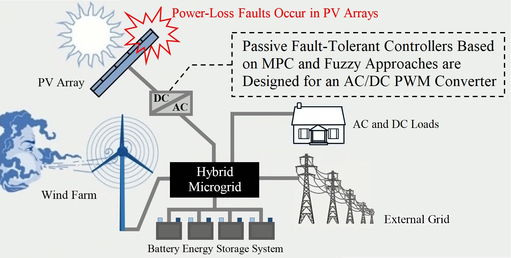
• A new design of hybrid microgrid benchmark with the integration of distributed renewable energy resources (wind farm and solar array) suitable for FTC investigations is considered in MATLAB/Simulink environment. This benchmark simulates the highly nonlinear dynamics of a hybrid AC/DC microgrid as well as the uncertainties and disturbances involved in different components.
• Severe power-loss faults due to open-circuit malfunctions at the string level in a PV array is modeled and investigated. Such faults can destabilize the operation of the entire microgrid which is indeed a low-inertia power grid in which any abrupt changes or severe faults in any location of the microgrid may have adverse impacts on other locations of the microgrid too.
• The applications of fuzzy logic and MPC techniques for designing PFTC schemes in order to tolerate and accommodate power-loss faults in a PV array at microgrid level are investigated. The results confirm that an appropriate FTC design for power electronic converters can effectively handle the fault effects and prevent their propagation throughout the microgrid.
• Abrupt connection and disconnection of dynamic loads is another critical issue which is considered. Basically, if not effectively handled, dynamic loads can easily destabilize microgrids especially the low-voltage ones. This issue is even more challenging during the severe power-loss faults since the required balance between demanded and generated powers can be broken and the microgrid becomes unstable. Such disturbances due to variations in dynamic loads besides severe power-loss faults are simultaneously considered and investigated in this paper.
• During FTC control design procedure, the application of windowed Fourier analysis is investigated for the first time in order to achieve more suitable input signal for control.
• The rest of this paper is organized as follows: Section 2 presents the considered microgrid benchmark model. PV array system modeling and its failure modes with their effects on the microgrid are discussed in Section 3. Design of PFTC schemes for an AC/DC PWM converter is described in Section 4. The simulation results are discussed and demonstrated in Section 5, and finally, conclusions and future works are presented in Section 6.

2. Microgrid Benchmark

This paper considers a group of interconnected dynamic loads and DERs based on renewable energy systems such as wind turbines and PV arrays, and also BESS to make a hybrid microgrid with AC and DC parts. Figure 1 shows the single-line diagram of the designed microgrid. As seen in the figure, the microgrid uses circuit breakers (CBs) and different types of power electronic converters for regulating the power flow inside the microgrid. In addition, the microgrid’s central controller (MGCC) is responsible for the efficient and reliable operation of the microgrid in both grid-connected and islanded modes. Taking into account the wide variations of operating conditions as well as possible uncertainties and disturbances, a detailed model of the proposed microgrid system is implemented in MATLAB/Simulink environment.

In the following paragraphs, the DERs implemented in the microgrid are briefly reviewed.

2.1. Wind Farm

The wind farm is a group of six wind turbines with induction generators (i.e., three-phase doubly fed induction generators (DFIGs)) with 1.5 megawatt (MW) output power. The captured wind power is converted into electricity by the generator and transmitted into the microgrid through the stator and rotor windings and an AC/DC/AC back-to-back converter. A detailed model of insulated-gate bipolar transistors (IGBT) voltage-sourced converters (VSC) is employed to model the dynamics of interactions between control and power systems. Three-phase power converters consisting of 6 switches (under a bridge configuration with 3 arms) are implemented. In addition, a wind conversion control system including rotor-side converter control, grid-side converter control and pitch angle control are used to regulate turbines output power, terminal voltage, and reactive power. More details about wind farm modeling and grid integration can be found in [27,28].

2.2. Solar Farm

The solar farm represents a PV array designed to generate 100 kW of nominal power from sunlight in normal conditions. A unidirectional DC/DC converter with an internal maximum power point tracking (MPPT) control (based on perturb and observe algorithm) together with a boost converter are designed for the integration of the PV array. The number of modules in a string and number of strings in the array are determined based on the design procedure in [6]. The designed PV array consists of 60 strings of modules that are connected in parallel, and each string itself includes 6 modules that are connected in series. The PV modules data are obtained from the U.S. National Renewable Energy Laboratory (NREL) [29]. This database uses the manufacturer’s datasheets that are measured under standard test conditions (STC) (i.e., $irradiance=1000 W/m^2$ and $temperature=25 °C$).

Table 1. Photovoltaic (PV) module data used in the benchmark.

Manufacturer	SunPower
Model number	SPR-415E-WHT-D
Module type	Monocrystalline
Cells per module $\left(N_{cell}\right)$	128
Maximum power $\left(W\right)$	414.801
Open circuit voltage $V_{oc}\left(V\right)$	85.3
Short circuit current $I_{sc}\left(A\right)$	6.0978
Voltage at maximum power point $V_{mp}\left(V\right)$	72.9
Current at maximum power point $I_{mp}\left(A\right)$	5.69
Temperature coefficient of $V_{oc}\left(\%/°C\right)$	−0.229
Temperature coefficient of $I_{sc}\left(\%/°C\right)$	0.030706

presents the considered module type and its relevant data used in the benchmark. Section 3 provides more details about the PV array, its modeling, and fault/failure modes.

2.3. BESS

Energy storage systems such as BESS are necessary components of microgrids in order to address the intermittent behavior of renewable energy resources and their induced fluctuations on the output power, [30]. In general, both power quality and reliability in microgrids can be improve by using energy storage systems. By storing electricity when the generated power is more than demand (consumed power), the microgrid can continue its operation even in the absence of renewable resources such as wind or sun. Therefore, supplying the loads in peak hours and meeting the demand with a continuous power are facilitated. Moreover, the presence of BESS in microgrids improves the power quality through providing better frequency and voltage control capabilities. In the proposed benchmark, the BESS is modelled as a dynamic system based on a rechargeable lithium-ion battery model according to the method described in [31]. Additionally, a converter (i.e., bidirectional DC/DC converter) equipped with a controller is designed for the integration of battery to the microgrid.

3. PV Array Modeling and Fault Analysis

Before FTC design, it is essential to describe the system model, possible fault/failure modes, and also the effects of each fault. In a microgrid, faults may occur in different components including transmission lines and cables, power electronic equipment, distributed energy resources, and sensing devices. The focus of this paper is on power-loss faults in PV arrays and their adverse effects on microgrid operation. The following subsections provide more information about modelling of PV arrays and their possible fault/failure modes and effects.

3.1. PV Array Modeling

Indeed, the output power of a PV array relates to the solar radiation, ambient temperature, and the number of cells and modules in the array. The PV array model uses a single-diode equivalent circuit model with five parameters to simulate the nonlinear current-voltage (I–V) characteristics of the PV array that depend on the irradiance and the temperature [32]. These parameters include a dependent current source $I_{ph}$ (photovoltaic current), series resistance $R_s$, shunt resistance $R_{sh}$, diode saturation current $I_0$, and diode ideality factor $A$. The mentioned model is shown in Figure 2a. Moreover, Figure 2b shows the output I–V characteristics of the PV array with three highlighted remarkable points referred to as short circuit point $\left(0,I_{sc}\right)$, maximum power point $\left(V_{mp},I_{mp}\right)$, and open circuit point $\left(V_{oc},0\right)$. The above-mentioned model parameters must be determined to fit the module data. With respect to the considered module (defined in Table 1) under STC, the parameters are computed as $I_{sc,n}=6.0978 \mathrm{A}$, $I_{0,n}=7.1712\times {10}^{-13} \mathrm{A}$, $A=0.87223$, $R_s=0.5371 \mathsf{\Omega }$, and $R_{sh}=419.7813 \mathsf{\Omega }$.

A PV array consists of $N_p$ parallel PV strings each including $N_s$ modules of PV connected in series. The output PV current $I_{PV}$ as a function of output PV voltage $V_{PV}$, the solar radiation $G \left(\mathrm{W}/{\mathrm{m}}^2\right)$, and the temperature $T \left(K\right)$ is given by [33]:

$$I_{PV}=N_p{I}_{ph}-N_p{I}_0\left[exp\left(\frac{q\left(V_{PV}+I_{PV}{R}_s\left(\frac{N_s}{N_p}\right)\right)}{KTA{N}_s}-1\right)\right]-\frac{V_{PV}+I_{PV}{R}_s\left(\frac{N_s}{N_p}\right)}{R_{sh}\left(\frac{N_s}{N_p}\right)}$$

(1)

where $I_{ph}$ is the photovoltaic current, $q$ is the charge of electron, and $K$ is the Boltzmann’s constant. This equation originates the I–V curve shown in Figure 2b.

In Equation (1), the dependence of photovoltaic current on the irradiance and temperature is described by [34]:

$$I_{ph}=\left[I_{sc,n}+k_c\left(T-T_n\right)\right]\frac{G}{1000}$$

(2)

where $I_{sc,n}$ is the short circuit current at STC, $k_c$ is the temperature coefficient of $I_{sc}$, and $T_n$ is the nominal temperature. The diode saturation current $I_0$ can be expressed in terms of $T$ as follows [34]:

$$I_0=I_{0,n}{\left(\frac{T}{T_n}\right)}^{3}exp\left[\frac{q{E}_g}{AK}\left(\frac{1}{T_n}-\frac{1}{T}\right)\right]$$

(3)

where $I_{0,n}$ is the nominal saturation current and $E_g$ is the semiconductor’s bandgap energy.

In the event of faults in a PV array, the output power $P_{PV}=I_{PV}\times V_{PV}$ decreases and the faulty array attains different I-V characteristic curves depending on the type of faults. In [35,36], a comprehensive study on PV array faults and their effects on the output characteristic curves of PV system is presented. The next section briefly discusses the power-loss faults in PV arrays and their effects on microgrids.

3.2. Power-Loss Faults in PV Arrays

In normal operating conditions, the output power of a PV array is very close to the predicted output power. However, during the faulty operation, the output power deviates from its nominal value and the performance of the array decreases. Some papers on various faults and detection techniques in PV arrays can be found in [12,37,38,39,40]. In PV arrays, faults may occur in cell, module or string level due to degradation, overheating, damaged panels, fractured glass, or open/short circuits [41]. Reduction in the PV output power is the main consequence of the mentioned failures. Basically, at the microgrid level, the required balance between the demanded power and the generated power must be maintained. Otherwise, any sudden power imbalance leads to a dangerous fluctuation in the voltage and current signals, and accordingly, an unpermitted deviation in the frequency of the microgrid’s AC part. Therefore, a severe fault in a PV array accompanied by a sudden reduction in the output power will adversely affect the current and voltage signals, and also the frequency and voltage stability of the microgrid.

One of the frequent faults in a PV array is indeed the “open-circuit fault” that occurs because of various reasons such as cables or joints breakdown, falling objects on the panels, corrosion, or manufacturing defects [35]. Figure 3 shows two open-circuit (or disconnection) faults indicated by “Fault 1” and “Fault 2” in one string and two strings of a PV array, respectively. The same figure also shows the characteristic curves of these faults with respect to those related to the same array but in normal condition without any faults. As one can see, the open-circuit voltage (under fault-free and also faulty conditions) remains almost the same. On the other hand, the short-circuit current and maximum power decrease as the number of disconnected strings increases [35,36]. This fault can be easily modeled by reducing the number of parallel PV strings, $N_p$, in Equation (1).

In the proposed microgrid benchmark model, a bidirectional power converter (i.e., AC/DC PWM converter) is used for connecting the DC part of the microgrid into the AC part (see Figure 1). This converter uses a bank of IGBTs with PWM signal generator to convert the DC power into AC, and also stabilize the DC bus voltage at 460 V (the nominal voltage for DC bus in the microgrid). A severe open-circuit fault in the PV array reduces the output power and has adverse impacts on the output voltage and current signals, the stability of the DC voltage, the power flow between DC part and AC part, and the measured frequency of the microgrid. These adverse impacts become exacerbated in the presence of disturbances such as abrupt loads disturbances. Nevertheless, an FTC for the AC/DC PWM converter can enhance the microgrid operations in case of power-loss faults and obtain an acceptable performance.

It is worth mentioning that the output power loss is a common consequence of all types of faults in PV arrays. Having said that, the PFTC schemes proposed in the following section can tackle any types of faults in PV arrays since the purpose of the PFTC schemes is to regulate the power flow using AC/DC PWM converter in the event of severe PV output power losses under any fault conditions in general.

4. Fault-Tolerant Control Design for AC/DC PWM Converter

In hybrid microgrids, the DC power generated in the PV array must be converted into AC power at an appropriate frequency (i.e., 50 or 60 Hz). Therefore, power converters are used to improve the integration and controllability of renewable energy resources. Here, an AC/DC PWM converter is used to connect the DC part of the microgrid to the AC part, and regulate the power flow between two parts, and stabilize the predefined DC bus voltage. The single-phase AC/DC power electronic converter includes a bank of IGBTs (i.e., 4 IGBTs in H-bridge topology) that uses PWM signals from the controller. Figure 4 shows the implemented block diagram of the microgrid’s DC part (i.e., the part shown with the red dashed box in Figure 1). This block diagram contains a single-diode model of the PV array, the DC/DC boost converter equipped with MPPT control unit, the high voltage DC bus, the BESS with bidirectional DC/DC converter, the AC/DC PWM converter for connecting the DC part to the AC grid, two dynamic AC loads, and a multi-winding transformer for three-phase integration. Additionally, the figure includes the AC/DC PWM converter controller with relevant feedback signals and the reference value for $V_{dc}$ (denoted by $V_{dc,ref}$).

As seen in the figure and will be discussed in the following sections, the converter’s baseline (default) controller is a conventional control system based on proportional-integral (PI) control which is substituted by the proposed PFTC schemes based on FGS and MPC techniques. The baseline controller only relies on three measured inputs, while the PFTC schemes employ two additional measured signals including PV output voltage $V_{PV}$ and current $I_{PV}$. In more detail, Figure 5 shows the control loop of the baseline controller which uses the secondary voltage $V_{sec}$ and current $I_{sec}$ of the transformer as well as the high-DC voltage $V_{dc}$ to keep the bus voltage within the safe limits. As shown in Figure 5, the converter’s control loop includes a PWM signal generator and two PI controllers (i.e., a voltage controller and a current controller) in a feedforward path. Based on Ziegler-Nichols tuning rule, the obtained gains are $\left\{K_{p,1}=300, K_{I,1}=3500\right\}$ and $\left\{K_{p,2}=0.1, K_{I,2}=25\right\}$ for the voltage and current controllers, respectively. The baseline voltage controller is described by:

$$U_c\left(t\right)=K_{P,n}{e}_{dc}\left(t\right)+K_{I,n}{{\displaystyle \int }}_0^t{e}_{dc}\left(\tau \right)d\tau$$

(4)

in which $U_c\left(t\right)$ is the control signal, $e_{dc}\left(t\right)=V_{dc}-V_{dc,ref}$ is the voltage tracking error, and $V_{dc,ref}$ is the reference voltage. Additionally, the nominal values for proportional and integral gains are defined as $K_{P,n}$ and $K_{I,n}$, respectively.

This paper aims at designing two PFTC schemes using FGS and MPC techniques to substitute for the voltage controller in Equation (4) with the purpose of accommodating the PV power-loss faults and maintaining the microgrid’s safe operation during severe malfunctions in the PV array. In the following subsections, the proposed control schemes are separately designed and implemented to control AC/DC PWM converter.

4.1. PFTC Design using FGS

In this section, FGS technique is used to design a PFTC scheme for the AC/DC PWM converter. Figure 6 shows the general structure of the proposed PFTC scheme using FGS. Compared with the baseline PI control structure (shown in Figure 5), the PI voltage controller is substituted by an FGS-PI control system and two additional feedback signals ($V_{PV}$ and $I_{PV}$) are used to estimate the PV array’s output power at each time instant. As seen in Figure 6, the FGS-PI controller has two inputs including ${\widehat{P}}_{PV}$ and $\left|F_{e_{dc}}\right|$. Here, ${\widehat{P}}_{PV}$ is the difference between the obtained and nominal (desired) output powers from the PV array, while $\left|F_{e_{dc}}\right|$ is a positive magnitude obtained from the windowed Fourier analysis of the tracking error signal $e_{dc}$. Indeed, in a hybrid AC/DC microgrid, the DC part is influenced by the AC part. Therefore, measured DC signals may contain high-frequency components due to the AC integration and noise in sensors [15]. In this paper, a novel approach based on windowed Fourier analysis is introduced in order to eliminate possible noise on the error signal and achieve a well-processed signal that can be easily used by fuzzy inference rules. Another reason for using Fourier analysis of the signal relates to its capability to clearly represent the divergence of the harmonics-contaminated signals from their nominal values during the microgrid operation. For instance, when there is a severe AC load connection or disconnection, the resulting impacts can be seen as fluctuations in the performance of microgrid’s DC part. Such fluctuations will be more catastrophic, especially during the faulty operation of the microgrid when controlled signals can oscillate unstably and diverge from their desired values.

4.1.1. Windowed Fourier Analysis

The Fourier block in Figure 6 implements a Fourier analysis of the input signal (i.e., the high-DC voltage tracking error signal $e_{dc}$) over one-cycle running window of the fundamental frequency of the signal. A signal $f\left(t\right)$ can be stated by Fourier series as follows:

$$f\left(t\right)=\frac{a_0}{2}+{\displaystyle \sum }_{n=1}^{\infty }\left(a_n\cos \left(n\omega t\right)+b_n\sin \left(n\omega t\right)\right)$$

(5)

where $\omega =\frac{2\pi }{\lambda }$ and $f\left(t\right)$ are integrable on an interval of length $\lambda$ (which is the period of Fourier series), $a_n$ and $b_n$ are Fourier coefficients, and $n$ is the rank of the harmonics ($n=1$ represents the fundamental component). Without loss of generality, the magnitude and phase of the harmonic components are defined as follows:

$$\left|u\right|=\sqrt{a_n^2+b_n^2}$$

(6)

$$\angle u=\mathrm{atan}\left(\frac{a_n}{b_n}\right)$$

(7)

where

$$a_n=\frac{2}{\lambda }{{\displaystyle \int }}_{t-\lambda }^{t}f\left(t\right)\cos \left(n\omega t\right)dt$$

(8)

$$b_n=\frac{2}{\lambda }{{\displaystyle \int }}_{t-\lambda }^{t}f\left(t\right)\sin \left(n\omega t\right)dt$$

(9)

$$\lambda =\frac{1}{f_1}, f_1:fundamental frequency$$

(10)

The output of the Fourier block (denoted by $\left|u\right|$) returns the magnitude of the harmonic components. As shown in Figure 6, the input of the Fourier block is the high-DC voltage tracking error signal $e_{dc}\left(t\right)=V_{dc}-V_{dc,ref}$, and the output $\left|u\right|=\left|F_{e_{dc}}\left(k\right)\right|$, that is a positive value, is used by the FGS-PI controller. For instance, Figure 7a shows $e_{dc}\left(t\right)$ signal during the fault-free operation of microgrid. As seen in this figure, the sign of the error signal varies with a high-frequency due to the integration to the microgrid’s AC part or uncertain measurements (that can be worsened by sensor degradation). Figure 7b shows the Fourier magnitude of the error signal. As observed in the figure, the obtained signal from the Fourier block is smooth and also caries useful information about dynamic loads (i.e., whenever the microgrid’s loads vary, the Fourier magnitude of the error signal increases). Such a processed signal is obtained in real-time and can be effectively utilized by the fuzzy inference rules. Therefore, the PFTC scheme using FGS technique that employs the windowed Fourier analysis can achieve well-processed signals from noise-contaminated signals. Then, further considerations can be applied through the appropriate selection and distribution of membership functions and fuzzy rules inside the fuzzy inference mechanism itself.

4.1.2. FGS-PI Control

The baseline PI controller in Equation (4) (i.e., the PI voltage controller shown in Figure 5) uses an individual input that is the high-DC voltage tracking error $e_{dc}$. However, the proposed PFTC scheme uses two inputs including the Fourier magnitude of the error signal denoted by $\left|F_{e_{dc}}\left(k\right)\right|$ and the difference between PV output power $P_{PV}\left(k\right)$ and nominal power $P_{PV,n}$ at time step $k$ (i.e., ${\widehat{P}}_{PV}\left(k\right)=P_{PV,n}-P_{PV}\left(k\right)$ and $P_{PV}\left(k\right)=I_{PV}\left(k\right)\times V_{PV}\left(k\right)$). These inputs allow for a better understanding of the system’s dynamics to enable PFTC design.

In the presented gain-scheduling technique, a fuzzy inference mechanism is employed to carry out the online modification of proportional and integral gains in the baseline PI controller. In addition, two simple linear transformations are defined under which the tuning of gains are applied as follows:

$$K_{P,opt}\left(k\right)=K_{P,min}+\left(K_{P,max}-K_{P,min}\right)K_{P,f}\left(k\right)$$

(11)

$$K_{I,opt}\left(k\right)=K_{I,min}+\left(K_{I,max}-K_{I,min}\right)K_{I,f}\left(k\right)$$

(12)

where $K_{P,f}\left(k\right)$ and $K_{I,f}\left(k\right)$ are normalized values between zero and one, and $\left[K_{P,min},K_{P,max}\right]$ and $\left[K_{I,min},K_{I,max}\right]$ are prescribed ranges for proportional and integral gains respectively. The above ranges are given by [42]:

$$K_{P,max}=0.6K_u$$

(13)

$$K_{P,min}=0.32K_u$$

(14)

where $K_u$ is the oscillation gain at the stability limit using P-control. Accordingly, the range of integral gain is obtained based on the following equation in which $T_i$ is the integral time constant:

$$K_{I,opt}=\frac{K_{P,opt}}{T_i}$$

(15)

Although the above equations provide an estimation for each range, more simulation studies as well as experiments may still be required to achieve a desirable control performance. The $K_{P,f}\left(k\right)$ and $K_{I,f}\left(k\right)$ parameters in Equations. (11) and (12) are obtained in real time using a set of linguistic if-then rules in the following form:

$$\begin{array}{cc}Rule i:\hfill & \\ \hfill & \mathit{I}\mathit{f} {\widehat{P}}_{PV}\left(k\right) is A_i \mathit{a}\mathit{n}\mathit{d} \left|F_{e_{dc}}\left(k\right)\right| is B_i, \hfill \\ \hfill & \mathit{t}\mathit{h}\mathit{e}\mathit{n} K_{P,f}\left(k\right) is C_i \mathit{a}\mathit{n}\mathit{d} K_{I,f}\left(k\right) is D_i\hfill \end{array}$$

(16)

where $A_i$, $B_i$, $C_i$, and $D_i$ (with $i=1,2,\dots ,M$) are fuzzy sets corresponding to ${\widehat{P}}_{PV}\left(k\right)$, $\left|F_{e_{dc}}\left(k\right)\right|$, $K_{P,f}\left(k\right)$, and $K_{I,f}\left(k\right)$, respectively. The triangular membership functions for input signals $\left|F_{e_{dc}}\left(k\right)\right|$ and ${\widehat{P}}_{PV}\left(k\right)$ are shown in Figure 8a. In this figure, the fuzzy membership function “S” stands for small, “M” for medium, “B” for big, “SP” for small plus, “MP” for medium plus, “BP” for big plus, and “ZO” for approximately zero. The generalized bell-shaped membership functions used for the outputs $K_{P,f}\left(k\right)$ and $K_{I,f}\left(k\right)$ are scaled from 0 to 1, and are in the following form:

$$\mu \left(x\right)=\frac{1}{1+{\left|\frac{x-c}{a}\right|}^{2b}}$$

(17)

where $a$, $b$, and $c$ are the function parameters. The above equation presents a nonlinear mapping between $\mu$ (the degree of membership) and $x=\left(K_{P,f}\left(k\right) \mathrm{or} K_{I,f}\left(k\right)\right)$. Figure 8b shows the output membership functions.

The complete set of rules shown in

Table 2. Fuzzy Rules For $K_{P,f}/K_{I,f}$ in $Rule i$.

					$\left|{\mathit{F}}_{{\mathit{e}}_{\mathit{d}\mathit{c}}},\left(\mathit{k}\right)\right|$
		ZO	S	SP	M	MP	B	BP
	ZO	ZO/ZO	ZO/ZO	ZO/ZO	ZO/ZO	ZO/ZO	ZO/ZO	ZO/ZO
	S	S/ZO	S/ZO	S/ZO	SP/S	SP/S	SP/S	SP/S
	SP	SP/SP	SP/SP	M/M	M/M	MP/M	MP/MP	MP/MP
${\widehat{\mathit{P}}}_{\mathit{P}\mathit{V}}\left(\mathit{k}\right)$	M	M/SP	M/M	MP/M	MP/MP	MP/MP	B/MP	B/MP
	MP	MP/MP	MP/MP	MP/MP	B/MP	B/B	B/B	B/B
	B	B/B	B/B	B/B	B/B	BP/BP	BP/BP	BP/BP
	BP	BP/BP	BP/BP	BP/BP	BP/BP	BP/BP	BP/BP	BP/BP

represents those implemented in Equation (16). The rules are formulated based on an expert’s knowledge. In this paper, the minimum operator is used to implement the logic AND, and the center-of-area method is used to represent the defuzzification as follows [42]:

$$K_{P,f}\left(k\right)=\frac{{{\displaystyle \sum }}_{i=1}^M{\mu }_i{K}_{P,f}^i\left(k\right)}{{{\displaystyle \sum }}_{i=1}^M{\mu }_i}$$

(18)

$$K_{I,f}\left(k\right)=\frac{{{\displaystyle \sum }}_{i=1}^M{\mu }_i{K}_{I,f}^i\left(k\right)}{{{\displaystyle \sum }}_{i=1}^M{\mu }_i}$$

(19)

where $K_{P,f}^i$ and $K_{I,f}^i$ are respectively the values of $K_{P,f}\left(k\right)$ and $K_{I,f}\left(k\right)$ relating to ${\mu }_i$ (the degree of membership for the $i$th rule). The equivalent input-output presentations of the FGS system for $K_{P,f}\left(k\right)$ and $K_{I,f}\left(k\right)$ are shown in Figure 9.

4.2. PFTC Design using MPC

In this section, MPC technique is used to design a PFTC scheme for the AC/DC PWM converter. Figure 10 shows the general structure of the proposed PFTC scheme using MPC. Compared with the baseline PI control structure (shown in Figure 5), the PI voltage controller is substituted by an MPC system and two additional feedback signals ($V_{PV}$ and $I_{PV}$) are used to estimate the PV array’s output power at each time instant. Therefore, the overall feedback signals used here are similar to those used for the designed PFTC scheme using FGS. However, compared with the FGS system in the former scheme, the root mean square (RMS) values of the secondary current and voltage of transformer ($I_{s,RMS}$, $V_{s,RMS}$) are also used by the MPC system (in addition to $V_{dc}$, $V_{dc,ref}$, $V_{PV}$, and $I_{PV}$). Indeed, $I_{s,RMS}$, $V_{s,RMS}$, $I_{PV}$, and $V_{PV}$ are considered as disturbances for the plant prediction model in MPC. It should be emphasized that the mentioned RMS inputs carry useful information about the dynamic loads (Load 1 and Load 2 in Figure 4). In the microgrid, dynamic loads can be unpredictable and the use of the mentioned RMS signals helps handle the possible uncertainties attached to the loads’ profiles. Additionally, due to the presence of the PV array in the microgrid, which is a largely intermittent energy resource, the proposed MPC controller considers the output current and voltage of the PV array as disturbances for the plant prediction model. As a result, the proposed scheme responds more robustly to uncertainties in the loads and generation.

During the grid-connected mode of operation, the output current of the PV array is directly proportional to the output current of the AC/DC converter since $V_{dc}$ is fixed using the AC/DC converter (see Figure 4). If a power-loss fault occurs in the PV array while the microgrid receives power from the grid (due to the loads connections), the RMS value of the secondary current $I_{s,RMS}$ increases that means more power is needed from the grid. Conversely, if a power-loss fault occurs in the PV array while the microgrid is exporting power to the grid, $I_{s,RMS}$ decreases and that means less power is sent to the grid. As a result, the MPC controller, which is responsible for regulating the power flow between AC and DC parts of the microgrid, uses the implicit information of faults in a passive procedure. Therefore, the whole PFTC scheme using MPC can effectively control the power flow in the microgrid during the faulty operation of the PV array and can accommodate the effects of power-loss faults.

In the MPC system, an optimal control problem is solved over a finite horizon at each sampling time. The solution depends on a prediction model, predefined constraints, and the optimization of a quadratic cost function. Therefore, provided that the prediction model is accurate enough and the quadratic cost function and predefined constraints show the exact performance objectives, the designed MPC achieves a near-optimal result. The following sections provide more details about the proposed MPC system.

4.2.1. Prediction Model

The prediction model used in the MPC system for prediction and state estimation consists of a plant model and a noise model. The plant model is a sampled linear time-invariant (LTI) system whose inputs include the command signal $u\left(k\right)$ and the disturbance $u_v\left(k\right)={\left[I_{s,RMS},V_{s,RMS},I_{PV},V_{PV}\right]}^T$, and described by [43]:

$$\left\{\begin{array}{c}{x}_p\left(k+1\right)=A_p{x}_p\left(k\right)+B_{p,mv}u\left(k\right)+B_{p,v}{u}_v\left(k\right)\\ y_p\left(k\right)=C_p{x}_p\left(k\right)+D_{p,mv}u\left(k\right)+D_{p,v}{u}_v\left(k\right)\end{array}\right.$$

(20)

where $A_p\left(k\right)$, $B_{p,mv}\left(k\right)$, $B_{p,v}\left(k\right)$, $C_p\left(k\right)$, $D_{p,mv}\left(k\right)$, and $D_{p,v}\left(k\right)$ are constant state-space matrices. Additionally, $x_p\left(k\right)$, $u\left(k\right)$, $u_v\left(k\right)$ and $y_p\left(k\right)$ are the state vector, the command signal, disturbance and the output of the plant model, respectively. The plant model is linearized as a third order system using a system identification process described in Section 5.4. Not only is this model accurate enough to capture the most significant dynamics of the microgrid, but it is also simple enough to solve the optimization problem in MPC.

To implement a well-designed prediction model, a noise model is also considered as a discrete-time LTI system by:

$$\left\{\begin{array}{c}{x}_n\left(k+1\right)=A_n{x}_n\left(k\right)+B_n{u}_n\left(k\right)\\ y_n\left(k\right)=C_n{x}_n\left(k\right)+D_n{u}_n\left(k\right)\end{array}\right.$$

(21)

where $A_n\left(k\right)$, $B_n\left(k\right)$, $C_n\left(k\right)$, and $D_n\left(k\right)$ are constant state-space matrices, while $x_n\left(k\right)$, $u_n\left(k\right)$, and $y_n\left(k\right)$ are the state vector, the input, and the output of the noise model, respectively.

The state vector of the prediction model can be defined as $x_c\left(k\right)={\left[x_p\left(k\right),x_n\left(k\right)\right]}^T$, where $x_c$ is the controller state (comprising $n_{xp}+n_{xn}$ state variables), $x_p$ is the plant model state vector (of the length of $n_{xp}$) and $x_n$ is the noise model state vector (of the length of $n_{xn}$). Combination of the models in Equations (20) and (21) yields the generalized state-space model:

$$\left\{\begin{array}{c}{x}_c\left(k+1\right)=A{x}_c\left(k\right)+B{u}_o\left(k\right)\\ y\left(k\right)=C{x}_c\left(k\right)+D{u}_o\left(k\right)\end{array}\right.$$

(22)

where the prediction model input is $u_o\left(k\right)={\left[u\left(k\right),u_v\left(k\right),u_n\left(k\right)\right]}^T$, the output is $y\left(k\right)=y_p\left(k\right)+y_n\left(k\right)$ and the constant matrices are:

$$\begin{gathered} A=\left[\begin{array}{cc}{A}_p& 0\\ 0& A_n\end{array}\right], B=\left[\begin{array}{ccc}{B}_{p,mv}& B_{p,v}& 0\\ 0& 0& B_n\end{array}\right], \\ C=\left[\begin{array}{cc}{C}_p& C_n\end{array}\right], D=\left[\begin{array}{ccc}{D}_{p,mv}& D_{p,v}& D_n\end{array}\right] \end{gathered}$$

(23)

The MPC system uses the generalized model in Equations (22) and (23) to estimate values of unmeasurable states required for prediction, and to predict how the controller’s manipulated variables (MV) adjustments will affect the plant’s future output.

4.2.2. State Estimation and Output Prediction

Since the true states of the model are not available to the controller, the steady-state Kalman filter is implemented. Indeed, the controller uses its current states, $x_c$, as the basis for predictions. At the beginning of the $k$th time step, the state of the controller is determined using Algorithm 1. Additionally, the MPC system requires the prediction of the plant output in order to solve the optimization problem. Then, at time step $k$, the output is predicted using Algorithm 2.

Algorithm 1. State estimation method used by MPC controller

1: Inputs: $\left\{x_c\left(k|k-1\right),u^{act}\left(k-1\right),u^{opt}\left(k-1\right),u_v\left(k\right) ,y\left(k\right),B_u, B_v,C_m,D_{mv},L,M\right\}$ $x_c\left(k|k-1\right)$: controller state estimation from previous time step $k-1$, $u^{act}\left(k-1\right)$: actual manipulated variable used from $k-1$ to $k$, $u^{opt}\left(k-1\right)$: optimal manipulated variable that was recommended by MPC to be used from $k-1$ to $k$, $u_v\left(k\right)$: current disturbances, $y\left(k\right)$: current measured plant output, $B_u,B_v$: columns of $B$ corresponding to $u\left(k\right)$ and $u_v\left(k\right)$, $C_m$: rows of $C$ corresponding to plant output, $D_{mv}$: rows and columns of $D$ corresponding to $u_v\left(k\right)$, $L,M$: constant Kalman gain matrices. 2: Outputs: $\{x_c\left(k|k\right)$, $u^{opt}\left(k\right),x_c\left(k+1|k\right)\}$ $x_c\left(k|k\right)$: controller state estimation at time step $k$, $u^{opt}\left(k\right)$: the MPC-recommended MV to be used between time steps $k$ and $k+1$, $x_c\left(k+1|k\right)$: controller state prediction for the time step $k+1$. 3: Variables: $\{x_c^{rev}\left(k|k-1\right)$, $e\left(k\right)\}$ $x_c^{rev}\left(k|k-1\right)$: revised $x_c\left(k|k-1\right)$, $e\left(k\right)$: error used in the procedure. 4: if $u^{act}\left(k-1\right)\ne u^{opt}\left(k-1\right)$ then 5: $x_c^{rev}\left(k|k-1\right)=x_c\left(k|k-1\right)+B_u\left[u^{act}\left(k-1\right)-u^{opt}\left(k-1\right)\right]$; 6: else 7: $x_c^{rev}\left(k|k-1\right)=x_c\left(k|k-1\right)$; 8: end if 9: $e\left(k\right)=y\left(k\right)-\left[C_m{x}_c^{rev}\left(k|k-1\right)+D_{mv}{u}_v\left(k\right)\right]$; 10: $x_c\left(k|k\right)=x_c^{rev}\left(k|k-1\right)+Me\left(k\right)$; // Update the controller state estimate 11: $u^{opt}\left(k\right)=solve\_QP\left(k\right)$; // Solve the QP problem at time step $k$ 12: $x_c\left(k+1|k\right)=A{x}_c^{rev}\left(k|k-1\right)+B_u{u}^{opt}\left(k\right)+B_v{u}_v\left(k\right)+Le\left(k\right)$.

Algorithm 2. Output variable prediction method used by MPC controller

1: Inputs: $\left\{p,x_c\left(k|k\right),u_v\left(k\right),u_v\left(k+i|k\right) ,A, B_u,B_v, C, D_v\right\}$ $p$: prediction horizon, $x_c\left(k|k\right)$: controller state estimates, $u_v\left(k\right)$: current disturbances, $u_v\left(k+i|k\right)$: projected future disturbances in which $\{i\in \mathbb{N},i<p\}$, $\mathbb{N}$: natural numbers set, $A, B_u,B_v, C, D_v$: constant matrices in the generalized model, where $B_u$, $B_v$ and $D_v$ show columns of $B$ and $D$ matrices relates to $u\left(k\right)$ and $u_v\left(k\right)$. 2: Output: $\left\{y\left(k+i|k\right)\right\}$ $y\left(k+i|k\right)$: the predicted noise-free plant output at any step in which $\left\{i\in \mathbb{N},i\le p\right\}$. 3: $x_c\left(k+1|k\right)=A{x}_c\left(k|k\right)+B_{u}u\left(k|k\right)+B_v{u}_v\left(k\right)$; // From the generalized model 4: for each $i\in \mathbb{N},1<i\le p$ do 5: $x_c\left(k+i|k\right)=A{x}_c\left(k+i-1|k\right)+B_{u}u\left(k+i-1|k\right)+B_v{u}_v\left(k+i-1|k\right)$ 6: end for 7: for each $i\in \mathbb{N},1\le i\le p$ do 8: $y\left(k+i|k\right)=C{x}_c\left(k+i|k\right)+D_v{u}_v\left(k+i-1|k\right)$ 9 end for

4.2.3. Optimization Problem

In MPC, an optimization problem (known as a quadratic programming (QP) problem) is solved at each time step. The obtained result determines the manipulated variables (MV) to be used until the next time step. The default performance index (or cost function) is the sum of four separate terms, each considering a specific performance aspect of the system: 1) output reference tracking; 2) MV tracking (i.e., the controller must maintain the MV approximately near the predefined target values); 3) MV move suppression (i.e., small MV moves are preferred); and 4) constraint violation. Note that constraint violations might be inevitable in practice, and thus, soft constraints help achieve a QP solution in such a case. In this regard, MPC system employs a variable ${\epsilon }_k$. Overall, each term includes proper weights to balance competing objectives [43]. The control action is achieved by solving the following QP problem:

$$J\left(Z_k\right)={\displaystyle \sum }_{i=0}^{p-1}\left({\displaystyle \sum }_{j=1}^{n_y}{\left(w_{i+1,j}^y\left[y_j\left(k+i+1|k\right)-r_j\left(k+i+1|k\right)\right]\right)}^2+{\displaystyle \sum }_{j=1}^{n_u}{\left(w_{i,j}^u\left[u_j\left(k+i|k\right)-u_{j,target}\left(k+i|k\right)\right]\right)}^2+{\displaystyle \sum }_{j=1}^{n_u}{\left(w_{i,j}^{\mathsf{\Delta }u}\left[u_j\left(k+i|k\right)-u_j\left(k+i-1|k\right)\right]\right)}^2\right)+{\rho }_{\epsilon }{\epsilon }_k^2$$

(24)

where the subscript “${\left(.\right)}_j$” denotes the $j$th component of a vector, and “$\left(k+i|k\right)$” shows the value predicted at time step $k+i$ based on the information at time step $k$. In addition, $y_j\left(k+i+1|k\right)$ is the predicted value of the $j$th output at the $\left(i+1\right)$th prediction horizon step, $r_j\left(k+i+1|k\right)$ is the reference value for the $j$th output at the $\left(i+1\right)$th prediction horizon step, $u_{j,target}\left(k+i|k\right)$ is the target value for the $j$th MV at the $i$th prediction horizon step, $w_{i+1,j}^y$ is the tuning weight for the $j$th plant output at the $\left(i+1\right)$th prediction horizon step, $w_{i,j}^u$ is the tuning weight for the $j$th MV at the $i$th prediction horizon step, and $w_{i,j}^{\mathsf{\Delta }u}$ is the tuning weight for the $j$th MV movement at the $i$th prediction horizon step. Other variables in Equation (24) include $p$, $m$, $n_y$, $n_u$, and $Z_k$ which are the prediction horizon, the control horizon, the number of plant output variables, the number of manipulated variables, and the QP decision, respectively. Indeed, the QP decision is given by:

$$Z_k^T=[\mathrm{\Delta }u{\left(k|k\right)}^T \mathrm{\Delta }u{\left(k+1|k\right)}^T \dots \mathrm{\Delta }u{\left(k+m-1|k\right)}^T \epsilon k]$$

(25)

where $k$ is the current time step.

The controller receives $u_{j,target}\left(k+i|k\right)$ values for the entire horizon. It uses the estimator to predict the outputs $y_j\left(k+i+1|k\right)$. These outputs depend on $Z_k$, $u_v$, and state estimates. At time step $k$, the controller’s state estimates and disturbances are available. Therefore, $J$ is only a function of $Z_k$.

MPC constraints are bounded by:

$$y_{j,min}\left(i\right)-{\epsilon }_k{V}_{j,min}^y\left(i\right)\le y_j\left(k+i+1|k\right)\le y_{j,max}\left(i\right)-{\epsilon }_k{V}_{j,max}^y\left(i\right), j=1,\dots ,n_y$$

(26)

$$u_{j,min}\left(i\right)-{\epsilon }_k{V}_{j,min}^u\left(i\right)\le u_j\left(k+i|k\right)\le u_{j,max}\left(i\right)-{\epsilon }_k{V}_{j,max}^u\left(i\right), j=1,\dots ,n_u$$

(27)

$$\mathrm{\Delta }{u}_{j,min}\left(i\right)-{\epsilon }_k{V}_{j,min}^{\mathrm{\Delta }u}\left(i\right)\le \mathrm{\Delta }{u}_j\left(k+i|k\right)\le \mathrm{\Delta }{u}_{j,max}\left(i\right)-{\epsilon }_k{V}_{j,max}^{\mathrm{\Delta }u}\left(i\right), j=1,\dots ,n_u$$

(28)

$$\mathrm{\Delta }u\left(k+h|k\right)=0$$

(29)

$${\epsilon }_k\ge 0$$

(30)

for all $i=0,\dots ,p-1$, $h=m,\dots ,p$, and with respect to the sequence of input increments $\left\{\mathrm{\Delta }u\left(k|k\right),\dots , \mathrm{\Delta }u\left(k-1+m|k\right)\right\}$ and the variable ${\epsilon }_k$. The MPC sets $u\left(k\right)=u\left(k-1\right)+\mathrm{\Delta }{u}^{*}\left(k|k\right)$, where $\mathrm{\Delta }{u}^{*}\left(k|k\right)$ denotes the first element of the optimal sequence. In the mentioned constraints, $\left\{y_{j,min}\left(i\right), y_{j,max}\left(i\right)\right\}$are respectively the lower bound and the upper bound for the $j$th output at the $i$th prediction horizon step, $\left\{u_{j,min}\left(i\right), u_{j,max}\left(i\right)\right\}$ are respectively the lower bound and the upper bound for the $j$th MV at the $i$th prediction horizon step, and $\left\{\mathsf{\Delta }{u}_{j,min}\left(i\right), \mathsf{\Delta }{u}_{j,max}\left(i\right)\right\}$ are respectively the lower bound and the upper bound for the $j$th MV movement at the $i$th prediction horizon step.

In Equations (26)–(28), the constraints on $y$, $u$, and $\mathsf{\Delta }u$ are relaxed by applying the variable ${\epsilon }_k\ge 0$. Additionally, the weight parameter ${\rho }_{\epsilon }$ penalizes the violation of the constraints. The vectors including $V_{j,min}^y\left(i\right)$, $V_{j,max}^y\left(i\right)$, $V_{j,min}^u\left(i\right)$, $V_{j,max}^u\left(i\right)$, $V_{j,min}^{\mathrm{\Delta }u}\left(i\right)$, and $V_{j,max}^{\mathrm{\Delta }u}\left(i\right)$ have non-negative elements. The $V$ parameters are similar to the weights used in the cost function but for constraint softening. In the proposed MPC, all the input constraints are hard and all the output constraints are soft.

Lastly, when computing $u\left(k\right)$, only $\mathrm{\Delta }u\left(k|k\right)$ is actually considered. The remaining samples $\mathrm{\Delta }u\left(k+i|k\right)$ are eliminated. At the next time step, $k+1$, a new optimization problem based on $y\left(k+1\right)$ will be solved. The optimization problem is solved using QP solver in MATLAB. The matrices associated with the QP problem are defined in [44].

5. Simulation Results

In this section, the simulation results are presented and discussed in order to demonstrate the effectiveness of the proposed PFTC schemes. Simulations have been carried out over 4 s in MATLAB/Simulink environment based on the microgrid benchmark described in Section 2. The DC bus voltage is supposed to be constant at 460 volts (V) in the grid-connected operation of the microgrid. The considered dynamic loads in Figure 4 include “Load 1” that is active during [0.5, 1.5] s and [2.5, 3.5] s (50 kW active power), and “Load 2” that is active during [1.0, 1.5] s and [3.0, 3.5] s (100 kW active power). The mentioned loads (Load 1 and Load 2) are supplied by the PV array (if possible) or by receiving additional power from the AC part of the microgrid (if an extra power is required). Moreover, it is assumed that the battery will be only connected when CB8 trips open (see Figure 1). The AC/DC PWM converter must regulate the power flow between AC and DC parts of the hybrid microgrid, and thereby, maintain the DC bus voltage at the desired value (i.e., 460 V). In the following sections, the performance of the three control schemes (i.e., the baseline PI control, PFTC using FGS, and PFTC using MPC) are firstly compared during the fault-free operation. Afterwards, two severe power-loss fault scenarios (i.e., 65% and 80% power-loss faults) in the PV array are considered and the effectiveness of the proposed PFTC schemes are compared.

5.1. Fault-Free Operation

This section investigates and compares the performances of three considered controllers in a fault-free operation. Figure 11 shows the PV array output power during the fault-free operation using the three mentioned controllers separately. As seen in the figure, the PV array is implemented to generate 100 kW of active power in normal conditions. Having said that, the small fluctuations in PV output power in Figure 11 at instants $0.5$, $1.0$, $1.5$, $2.5$, $3.0$, and $3.5$ s are due to the loads’ activities (variations) in the medium-voltage DC microgrid. Indeed, as already mentioned, Load 1 and Load 2 are the dynamic loads which connect or disconnect at different moments during the microgrid’s operation. For instance, Figure 11 also shows the zoomed-in plots of output power in two chosen time periods of [0.98, 1.18] and [1.48, 1.68] s in which the considered loads become connected and disconnected, respectively. The zoomed-in plots clearly show that although all controllers can handle the loads’ variations, the PFTC schemes, and especially the one using MPC, score relatively better control performances compared with the baseline PI control. Figure 12 shows the loads’ activities over 4 s. As one can be seen, at $t=1$ s, Load 1 is already active when Load 2 becomes connected, and at $t=1.5$ s, both loads become disconnected. As shown, all control schemes can meet the loads’ demanded powers under fault-free conditions.

Figure 13 shows the high-DC voltage regulated around its reference value of 460 V. All three controllers can effectively maintain the DC voltage under severe loads variations. Figure 13 also shows the zoomed-in plots of the responses in two chosen time periods. In order to quantitatively investigate the effectiveness of the control schemes, the mean and standard deviation (STD) values of the high-DC voltage signal in Figure 13 are provided in

Table 3. Quantitative performance comparison of controllers during fault-free operation.

	High-DC Voltage		Transformer Secondary Current
	Mean	STD	Mean	STD
Baseline PI Control	460.1123	5.7112	−5.5873	476.4369
PFTC using FGS	460.1114	5.665	−5.4916	476.4261
PFTC using MPC	460.0165	4.7919	−0.464	475.4873

. According to this table, the mean value for the performance under PFTC using MPC is closer to the desired value of 460 V while the STD value is less than those of the other two controllers. Therefore, the PFTC scheme using MPC scores the best results. With respect to the PFTC using FGS, the obtained fault-free results are almost the same as those from the baseline PI control. The reason for this mainly relates to the designed fuzzy rules in the FGS system which only schedule the PI gains when severe variations such as faults happen. Figure 14 shows the secondary current of the multi-winding transformer which connects the three-phase AC power from the wind farm to the considered AC loads (see Figure 4). One can clearly observe the moments of load variations in this figure. The mean and STD values of the secondary current are presented in Table 3.

As previously stated, the AC/DC PWM converter is used to regulate the power flow between the DC and AC parts of the hybrid microgrid. The active power $P \left[W\right]$ and reactive power $Q \left[VAR\right]$ associated with the periodic voltage and current signals are calculated over one cycle of the fundamental frequency (i.e., 60 Hz in the considered microgrid) using a running average window. The transmitted active and reactive powers through CB8 (see Figure 1) are illustrated in Figure 15. As observed from this figure, all controllers can finely satisfy the regulation of power flow under fault-free conditions. A phasor measurement unit (PMU) is used to measure the frequency of the AC part at 11-kV bus in the microgrid (see Figure 1). Figure 16 shows the measured frequency. This figure also verifies the overall effectiveness of all three controllers to regulate frequency under fault-free conditions.

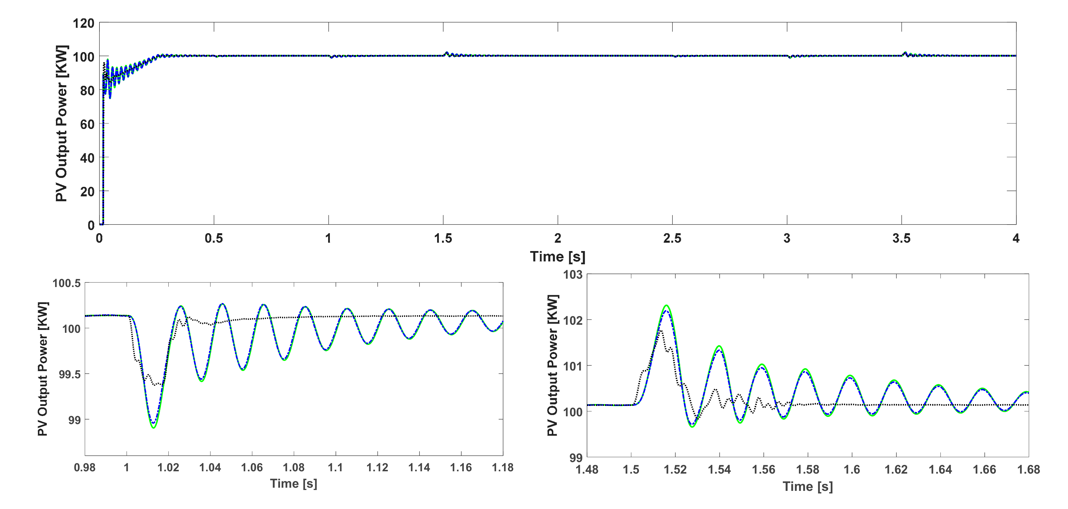
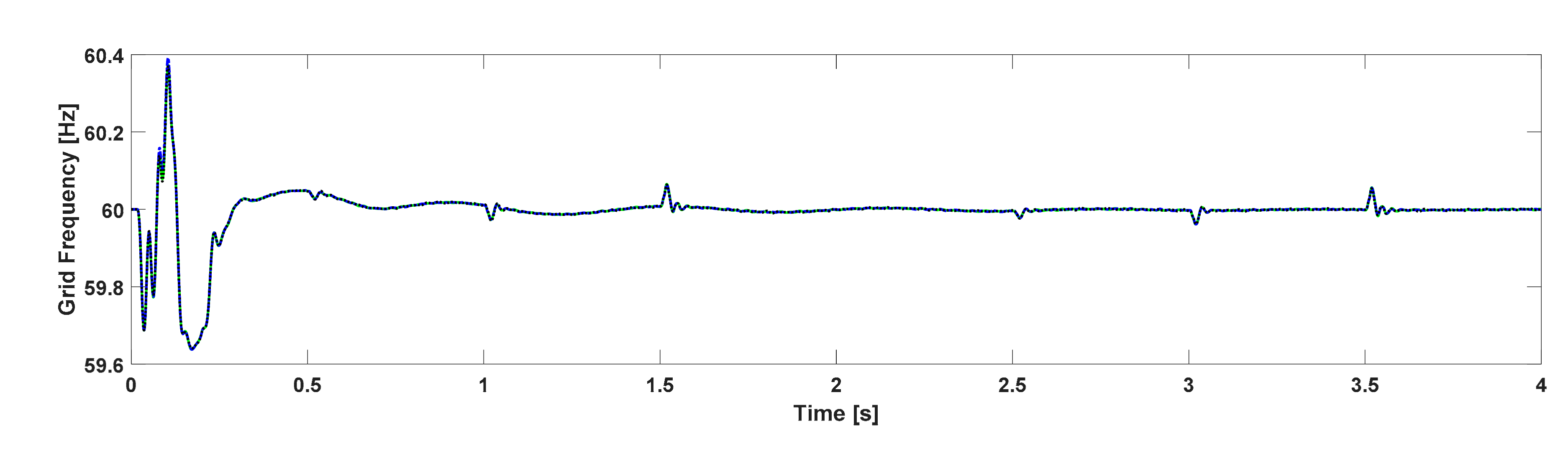
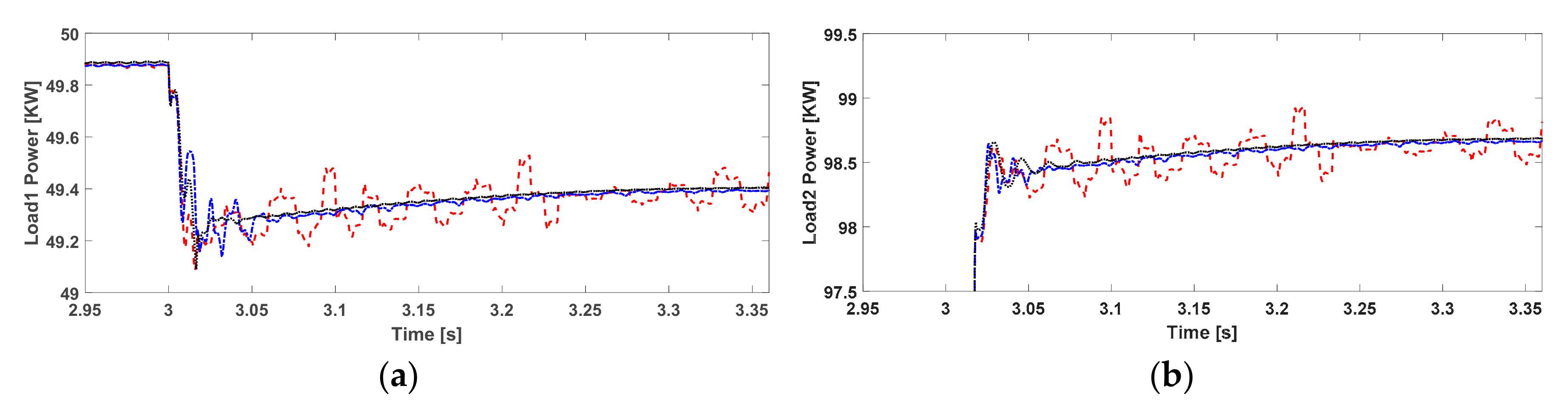
5.2. Faulty Operation under Fault Scenario 1 (65% Power Loss in PV Array)

The baseline PI control scheme is only robust against mild levels of power loss, or some types of faults which develop very incipiently (drift-wise). However, such a baseline control scheme (with constant (fixed) gains) cannot handle severe power-loss faults which cause catastrophic consequences due to their large magnitudes and instantaneous behaviors. In order to show the effectiveness of the proposed PFTC schemes under fault Scenario 1, an open-circuit power-loss fault is simulated in the PV array to start from $t=1$ s and continue to the end of the simulation. During this period of time, the output power of the PV array is substantially reduced to about 35 percent of its nominal power. Figure 17 shows the PV output power during fault-free and faulty operations with the three considered control schemes. As observed in this figure, the PV array’s output power is suddenly reduced when the fault occurs at $t=1$ s. In this scenario, both PFTC schemes handle the fault effects immediately, while the performance under the baseline PI control becomes unstable and the output power exhibits fluctuations.

It should be emphasized that because of the strong coupling among different components in the microgrid, any sudden change in any distributed components may destabilize the operation of the entire microgrid system especially during fault events. The presence of loads variations is a key challenge in the control of microgrids which must be considered. The zoomed-in plots in Figure 17 clearly show how the presence of dynamic loads during the microgrid’s faulty operation influence on the stability of the microgrid. As seen in the zoomed-in plots, when the loads abruptly change, the baseline PI control scheme cannot tolerate these disturbances, especially under fault conditions. However, the PFTC schemes can accommodate such effects and can maintain the microgrid’s safe operation. Figure 18 shows the power consumptions by Load 1 and Load 2 around $t=3$ s under the considered fault scenario. As observed in this figure, both the proposed PFTC schemes exhibit better performances compared with the baseline PI control.

Figure 19 shows the high-DC voltage regulated around its reference value of 460 V. As clearly shown in the figure, the high-DC voltage becomes intensively unstable under the baseline PI control. On the contrary, the two PFTC schemes can effectively control the DC bus voltage under both severe fault events and changes of dynamic loads. Figure 19 also shows the high-DC voltage in zoomed-in plots around two important moments of load change. As can be seen, for instance, when the fault becomes more severe at $t=2.5$ s and Load 1 is connected, the baseline PI control scheme is unable to maintain the system anymore, and thereby the DC bus voltage exceeds its safe range of variation.

The frequency of the AC part measured at 11-kV bus is shown in Figure 20. This figure also verifies the favorable effectiveness of the PFTC schemes in handling the fault effects as opposed to the baseline control scheme which cannot fully maintain the frequency. In addition, the transmitted active and reactive powers through CB8 are shown in Figure 21. As observed in these figures, more active power is required from the microgrid’s AC part as the PV power-loss fault becomes more severe. When the magnitude of fault increases, the baseline PI control scheme cannot handle the fault effects anymore. As a result, the active and reactive power flows oscillate heavily. Conversely, the PFTC schemes can effectively control and regulate the power flow in the whole range of power-loss faults with an acceptable performance.

5.3. Faulty Operation under Fault Scenario 2 (80% Power Loss in PV Array)

In the second scenario, a more severe open-circuit power-loss fault is considered due to which 80% of the PV array’s output power drops. As shown in Figure 22 including its zoomed-in plots, although the baseline PI control scheme exhibits some robustness against mild levels of power loss, it cannot handle the severe power-loss fault. It is observed that the PFTC scheme using FGS tolerates the severe power-loss fault until $t=3$ s before the fault fully reaches its 20% of the nominal power. Interestingly, the PFTC scheme using MPC can effectively tolerate the whole range of power loss in the PV array until the power loss is fully reached to the 20% of the array’s nominal power. However, it is worth mentioning that in terms of higher fault tolerance capabilities, this MPC’s favorable performance is obtained at a higher computational cost compared with the FGS technique which is easier to implement.

Abrupt connection/disconnection of loads, especially in low-voltage conditions, is a challenging control issue. As seen in Figure 22, shortly after $t=1.5$ s when both Loads are disconnected, the performance under the baseline PI control scheme becomes unstable due to the large load disturbance. It is also observed that at $t=3$ s, when the fault is more severe, the connection of Load 2 causes instability in the performance under the PFTC scheme using FGS. It is worth emphasizing that although the operation under the baseline PI control scheme became unstable before $t=3$ s, the resulted disturbance from the connection of Load 2 at $t=3$ s causes the system to return to its stable operation. However, this stability induced by the load connection would be temporary under the baseline PI control.

Figure 23 shows the high-DC voltage responses under the three considered control schemes. Using the baseline PI control scheme, the high-DC voltage deviates from its desired value (460 V) quickly at around $t=1.5$ s that is a long time before when the power loss level becomes severe (about 80%). After $t=1.5$ s, the operation under the baseline PI control remains unstable and the high-DC voltage exceeds its safe limits although the load variations help the system to operate around the desired high-DC voltage but at very short moments. Compared with the baseline PI control scheme, the PFTC scheme using FGS maintains the microgrid’s high-DC voltage for a longer time, but its control performance is lost after $t=3$ s (see Figure 23). Indeed, the only control scheme which can fully tolerate this harsher fault scenario (i.e., 80% power loss fault) is the PFTC scheme using MPC.

Figure 24 shows the secondary current of the transformer using the three controllers. In addition, Figure 25 shows the frequency of the microgrid’s AC part during the faulty operation. Overall, the entire simulation results indicate that both the proposed PFTC schemes exhibit better performances than the baseline PI control scheme. However, not only the overall effectiveness of the PFTC scheme using MPC is more noticeable under the fault-free operation, but also under the very severe power-loss fault conditions. In addition, the proposed MPC approach is successful in handling uncertainties of the dynamic loads during the microgrid’s both fault-free and faulty operations.

5.4. Identification and Validation of the MPC Model

As already discussed in Section 4, the PFTC scheme using MPC employs a plant model for prediction and optimization. The plant model is estimated as a third order system using prediction error minimization algorithm which is an iterative approach for black-box estimation [45]. This algorithm firstly initializes the model parameters using subspace method [46], and then an iterative search is used to minimize the prediction errors. A set of 10,000 measured data for every input and output were utilized to carry out the model identification and validation. The data were obtained from the simulation of the microgrid benchmark in its grid-connected mode. In order to measure the accuracy and fitting performance of the obtained model, the variance accounted for (VAF) index, Akaike’s final prediction error (FPE), as well as the mean squared error (MSE) are computed. The percentile VAF is computed by:

$$VAF=\left(1-\frac{cov\left(y_k-{\widehat{y}}_k\right)}{cov\left(y_k\right)}\right)100\%$$

(31)

in which $y_k$ is the $k$th output of the plant and ${\widehat{y}}_k$ is the estimated output by the model. In addition, the $cov$ refers to the covariance of the two vectors. Akaike’s FPE is computed by:

$$FPE=det\left(\frac{1}{n}{\displaystyle \sum }_1^{n}e\left(t,{\widehat{\phi }}_n\right){\left(e\left(t,{\widehat{\phi }}_n\right)\right)}^T\right)\left(\frac{1+\frac{m}{n}}{1-\frac{m}{n}}\right)$$

(32)

where $n$ is the number of values in the estimation data set, $e\left(t\right)$ is the vector of prediction error, $m$ is the number of estimated parameters, and ${\widehat{\phi }}_n$ is the estimated parameters vector. According to Akaike’s theory, an accurate model should have a small FPE. Lastly, the model’s MSE is computed by:

$$MSE=\frac{1}{n}{\displaystyle \sum }_{k=1}^n{\left(y_k-{\widehat{y}}_k\right)}^2$$

(33)

The obtained results are as follows: $VAF\left(\%\right)=96\%$, $FPE=0.0004189$, and $MSE=0.0004174$. From the data, the model is accurate enough for approximating and predicting the plant under control.

6. Conclusions and Future Works

This paper addressed the design and comparison of two passive fault-tolerant control schemes in a hybrid AC/DC microgrid. The proposed schemes are based on fuzzy gain-scheduling and model predictive control techniques. Both schemes do not require fault detection and diagnosis information (or explicit knowledge of faults), and tolerate fault effects due to power-loss faults in a solar PV array located in the microgrid in the presence of unknown uncertainties and load variations. Effective handling of severe power-loss faults as well as abrupt load variations prevents adverse impacts on the quality of power flow and the stability of microgrid as a whole.

Testing and simulation are carried out in MATLAB/Simulink environment. The considered microgrid benchmark involves wide variations in operating conditions and load uncertainties. Although the proposed scheme using fuzzy gain-scheduling technique showed almost the same fault-free performance as the one under the baseline PI control scheme, the passive fault tolerance provided by the fuzzy scheduling technique makes it superior to the baseline controller. However, the performance of the proposed scheme based on fuzzy gain-scheduling is not acceptable for highly severe power-loss faults. For this reason, another proposed scheme based on model predictive control technique is designed which can tolerate and accommodate more severe faults compared with its other counterparts. Numerical results clearly demonstrate the effectiveness of the proposed passive fault-tolerant control scheme using model predictive control for both fault-free and faulty conditions. In addition, thanks to the rapid increase in the computational power of modern microprocessors, the real-life application of model predictive control solutions is recently found more and more in power electronic applications.

At the end, it is worth mentioning that extending the proposed fault-tolerant control approaches to the accommodation of other types of faults such as sensor faults and developing the proposed microgrid benchmark to appropriate hardware-in-the-loop (HIL) equipment for real-time implementation of the control strategies remain as the future research topics. Moreover, other control strategies such as adaptive controllers and multiple model predictive controllers for multiple operating points can be investigated to obtain better results in the presence of disturbances. Designing active fault-tolerant control schemes with real-time control reconfiguration, robust fault detection and diagnosis at the microgrid level, and the application of fault-tolerant cooperative control techniques to microgrids are other interesting topics that need more investigations as well.

References

1. Farhangi, H. The path of the smart grid. IEEE Power Energy Mag. 2010, 8, 18–28. [Google Scholar] [CrossRef]
2. Lasseter, B. Microgrids distributed power generation. Power Eng. Soc. IEEE 2001, 1, 146–149. [Google Scholar] [CrossRef]
3. Lasseter, R.; Akhil, A.; Marnay, C.; Stephens, J.; Dagle, J.; Guttromsom, R.; Meliopoulous, A.S.; Yinger, R.; Eto, J. Integration of Distributed Energy Resources—The CERTS Microgrid Concept; Lawrence Berkeley National Lab. (LBNL): Berkeley, CA, USA, 2002; Available online: http://bnrg.eecs.berkeley.edu/~randy/Courses/CS294.F09/MicroGrid.pdf (accessed on 21 September 2020).
4. Parhizi, S.; Lotfi, H.; Khodaei, A.; Bahramirad, S. State of the art in research on microgrids: A review. IEEE Access 2015, 3, 890–925. [Google Scholar] [CrossRef]
5. Olivares, D.E.; Mehrizi-Sani, A.; Etemadi, A.H.; Cañizares, C.A.; Iravani, R.; Kazerani, M.; Hajimiragha, A.H.; Gomis-Bellmunt, O.; Saeedifard, M.; Palma-Behnke, R.; et al. Trends in microgrid control. IEEE Trans. Smart Grid 2014, 5, 1905–1919. [Google Scholar] [CrossRef]
6. Villalón, A.; Rivera, M.; Salgueiro, Y.; Muñoz, J.; Dragičević, T.; Blaabjerg, F. Predictive control for microgrid applications: A review study. Energies 2020, 13, 2454. [Google Scholar] [CrossRef]
7. Keyhani, A. Design of Smart Power Grid Renewable Energy Systems; John Wiley & Sons: Hoboken, NJ, USA, 2016. [Google Scholar]
8. Bae, S.; Kwasinski, A. Dynamic modeling and operation strategy for a microgrid with wind and photovoltaic resources. IEEE Trans. Smart Grid 2012, 3, 1867–1876. [Google Scholar] [CrossRef]
9. Oudalov, A.; Fidigatti, A. Adaptive network protection in microgrids. Int. J. Distrib. Energy Resour. 2009, 5, 201–226. Available online: http://www.microgrids.eu/documents/519.pdf (accessed on 21 September 2020).
10. Hosseinzadeh, M.; Rajaei Salmasi, F. Islanding Fault detection in microgrids—A survey. Energies 2020, 13, 3479. [Google Scholar] [CrossRef]
11. Zhang, Y.M.; Jiang, J. Bibliographical review on reconfigurable fault-tolerant control systems. Annu. Rev. Control 2008, 32, 229–252. [Google Scholar] [CrossRef]
12. Jadidi, S.; Badihi, H.; Zhang, Y.M. Fault diagnosis in microgrids with integration of solar photovoltaic systems: A review. In IFAC World Congress; Springer: Berlin/Heidelberg, Germany, 2020. [Google Scholar]
13. Badihi, H.; Jadidi, S.; Zhang, Y.M.; Su, C.Y.; Xie, W.F. AI-driven intelligent fault detection and diagnosis in a hybrid AC/DC microgrid. In Proceedings of the the 1st International Conference on Industrial Artificial Intelligence, Shenyang, China, 22–26 July 2019. [Google Scholar] [CrossRef]
14. Gholami, S.; Saha, S.; Aldeen, M. Fault tolerant control of electronically coupled distributed energy resources in microgrid systems. Int. J. Electr. Power Energy Syst. 2018, 95, 327–340. [Google Scholar] [CrossRef]
15. Jadidi, S.; Badihi, H.; Zhang, Y.M. Passive fault-tolerant control of PWM converter in a hybrid AC/DC microgrid. In Proceedings of the IEEE 2nd International Conference on Renewable Energy and Power Engineering (REPE), Toronto, ON, Canada, 2–4 November 2019. [Google Scholar] [CrossRef]
16. Prodan, I.; Zio, E.; Stoican, F. Fault tolerant predictive control design for reliable microgrid energy management under uncertainties. Energy 2015, 91, 20–34. [Google Scholar] [CrossRef] [Green Version]
17. Morato, M.M.; Mendes, P.R.; Normey-Rico, J.E.; Bordons, C. LPV-MPC fault-tolerant energy management strategy for renewable microgrids. Int. J. Electr. Power Energy Syst. 2020, 117, 105644. [Google Scholar] [CrossRef]
18. Hosseinzadeh, M.; Salmasi, F.R. Fault-tolerant supervisory controller for a hybrid AC/DC micro-grid. IEEE Trans. Smart Grid 2018, 9, 2809–2823. [Google Scholar] [CrossRef]
19. Lin, X.; Wang, Y.; Pedram, M.; Kim, J.; Chang, N. Designing fault-tolerant photovoltaic systems. IEEE Des. Test 2013, 31, 76–84. [Google Scholar] [CrossRef] [Green Version]
20. Boutasseta, N.; Ramdani, M.; Mekhilef, S. Fault-tolerant power extraction strategy for photovoltaic energy systems. Sol. Energy 2018, 169, 594–606. [Google Scholar] [CrossRef]
21. Kim, G.S.; Lee, K.B.; Lee, D.C.; Kim, J.M. Fault diagnosis and fault-tolerant control of DC-link voltage sensor for two-stage three-phase grid-connected PV inverters. J. Electr. Eng. Technol. 2013, 8, 752–759. [Google Scholar] [CrossRef] [Green Version]
22. Ribeiro, E.; Cardoso, A.J.; Boccaletti, C. Fault-tolerant strategy for a photovoltaic DC-DC converter. IEEE Trans. Power Electron. 2012, 28, 3008–3018. [Google Scholar] [CrossRef]
23. Guilbert, D.; Gaillard, A.; N’Diaye, A.; Djerdir, A. Power switch failures tolerance and remedial strategies of a 4-leg floating interleaved DC/DC boost converter for photovoltaic/fuel cell applications. Renew. Energy 2016, 90, 14–27. [Google Scholar] [CrossRef]
24. Li, Z.; Peng, T.; Zhang, P.F.; Han, H.; Yang, J. Fault diagnosis and fault-tolerant control of photovoltaic micro-inverter. J. Cent. South Univ. 2016, 23, 2284–2295. [Google Scholar] [CrossRef]
25. Boudjellal, B.; Benslimane, T. Open-switch fault-tolerant control of power converters in a grid-connected photovoltaic system. Int. J. Power Electron. Drive Syst. 2016, 7, 1294–1308. [Google Scholar] [CrossRef]
26. Guatam, V.; Illindala, M.S.; Sensarma, P. A fault tolerant controller for PV inverter in microgrid application. In Proceedings of the IEEE International Conference on Power Electronics, Drives and Energy Systems (PEDES), Chennai, India, 18–21 December 2018. [Google Scholar] [CrossRef]
27. Pena, R.; Clare, J.C.; Asher, G.M. Doubly fed induction generator using back-to-back PWM converters and its application to variable-speed wind-energy generation. IEE Proc. Electr. Power Appl. 1996, 143, 231–241. [Google Scholar] [CrossRef] [Green Version]
28. Miller, N.W.; Sanchez-Gasca, J.; Price, W.; Delmerico, R.W. Dynamic modeling of GE 1.5 and 3.6 MW wind turbine-generators for stability simulations. IEEE Power Eng. Soc. Gen. Meet. 2003, 3, 1977–1983. [Google Scholar] [CrossRef]
29. Blair, N.; Dobos, A.P.; Freeman, J.; Neises, T.; Wagner, M.; Ferguson, T.; Gilman, P.; Janzou, S. System Advisor Model, SAM 2014.1.14: General Description; National Renewable Energy Lab. (NREL): Golden, CO, USA, 2014. Available online: https://www.nrel.gov/docs/fy14osti/61019.pdf (accessed on 21 September 2020).
30. Poulek, V.; Dang, M.Q.; Libra, M.; Beránek, V.; Šafránková, J. PV Panel with Integrated Lithium Accumulators for BAPV Applications—One Year Thermal Evaluation. IEEE J. Photovolt. 2020, 10, 150–152. [Google Scholar] [CrossRef]
31. Tremblay, O.; Dessaint, L.A. Experimental validation of a battery dynamic model for EV applications. World Electr. Veh. J. 2009, 3, 289–298. [Google Scholar] [CrossRef] [Green Version]
32. Villalva, M.G.; Gazoli, J.R.; Filho, E.R. Comprehensive approach to modeling and simulation of photovoltaic arrays. IEEE Trans. Power Electron. 2009, 24, 1198–1208. [Google Scholar] [CrossRef]
33. Bouraiou, A.; Hamouda, M.; Chaker, A.; Sadok, M.; Mostefaoui, M.; Lachtar, S. Modeling and simulation of photovoltaic module and array based on one and two diode model using MATLAB/Simulink. Energy Procedia 2015, 74, 864–877. [Google Scholar] [CrossRef] [Green Version]
34. Zdiri, M.A.; Bouzidi, B.; Kahouli, O.; Abdallah, H. Fault detection method for boost converters in solar PV systems. In Proceedings of the The 19th IEEE International Conference on Sciences and Techniques of Automatic Control and Computer Engineering (STA), Sousse, Tunisia, 24–26 March 2019. [Google Scholar] [CrossRef]
35. Sabbaghpur Arani, M.; Hejazi, M.A. The comprehensive study of electrical faults in PV arrays. J. Electr. Comput. Eng. 2016, 8712960. [Google Scholar] [CrossRef]
36. Pei, T.; Hao, X. A fault detection method for photovoltaic systems based on voltage and current observation and evaluation. Energies 2019, 12, 1712. [Google Scholar] [CrossRef] [Green Version]
37. Madeti, S.R.; Singh, S.N. A comprehensive study on different types of faults and detection techniques for solar photovoltaic system. Sol. Energy 2017, 158, 161–185. [Google Scholar] [CrossRef]
38. Momeni, H.; Sadoogi, N.; Farrokhifar, M.; Gharibeh, H.F. Fault Diagnosis in Photovoltaic Arrays Using GBSSL Method and Proposing a Fault Correction System. IEEE Trans. Ind. Inform. 2020, 16, 5300–5308. [Google Scholar] [CrossRef]
39. Hare, J.; Shi, X.; Gupta, S.; Bazzi, A. A review of faults and fault diagnosis in micro-grids electrical energy infrastructure. IEEE Energy Convers. Congr. Expo. 2014, 3325–3332. [Google Scholar] [CrossRef]
40. Mellit, A.; Tina, G.M.; Kalogirou, S.A. Fault detection and diagnosis methods for photovoltaic systems: A review. Renew. Sustain. Energy Rev. 2018, 91, 1–17. [Google Scholar] [CrossRef]
41. Jadidi, S.; Badihi, H.; Zhang, Y.M. A review on operation, control and protection of smart microgrids. In Proceedings of the IEEE 2nd International Conference on Renewable Energy and Power Engineering (REPE), Toronto, ON, Canada, 2–4 November 2019. [Google Scholar] [CrossRef]
42. Zhao, Z.; Tomizuka, M.; Isaka, S. Fuzzy gain scheduling of PID controllers. IEEE Trans. Syst. ManCybern. 1993, 23, 1392–1398. [Google Scholar] [CrossRef] [Green Version]
43. Bemporad, A.; Ricker, N.; Owen, J.G. Model predictive control—New tools for design and evaluation. Am. Control Conf. 2004, 6, 5622–5627. [Google Scholar] [CrossRef]
44. Bemporad, A.; Ricker, N.; Morari, M. Model Predictive Control Toolbox for MATLAB: User’s Guide; The MathWorks, Inc.: Natick, MA, USA, 2014; Available online: http://fumblog.um.ac.ir/gallery/839/mpc_ug.pdf (accessed on 26 October 2020).
45. Ljung, L. System Identification: Theory for the User, 2nd ed.; Prentice Hall: Upper Saddle River, NJ, USA, 1999. [Google Scholar]
46. Overschee, P.V.; Moor, B.D. Subspace Identification for Linear Systems: Theory, Implementation, Applications; Springer: Boston, MA, USA, 1996; ISBN 978-1-4613-8061-0. [Google Scholar]
Figure 1. Single-line diagram of the considered hybrid microgrid.
Energies 13 05625 g001
Figure 2. Modelling and characteristic of a practical PV array: (a) Single-diode model, (b) I–V curve.
Energies 13 05625 g002
Figure 3. PV array configuration for open-circuit faults at the string level (measured under standard test conditions (STC)).
Energies 13 05625 g003
Figure 4. Schematic of the microgrid’s DC part.
Energies 13 05625 g004
Figure 5. Baseline control loop of the AC/DC pulse-width modulation (PWM) converter based on proportional-integral (PI) control.
Energies 13 05625 g005
Figure 6. Passive fault-tolerant control (PFTC) loop of the AC/DC PWM converter based on Fourier analysis and FGS-PI control.
Energies 13 05625 g006
Figure 7. Error signal characteristics during fault-free operation: (a) error signal, and (b) Fourier magnitude.
Energies 13 05625 g007
Figure 8. Membership functions in R u l e   i : (a) inputs, and (b) outputs.
Energies 13 05625 g008
Figure 9. Response surfaces: (a) K P , f k , and (b) K I , f k .
Energies 13 05625 g009
Figure 10. PFTC loop of the AC/DC PWM converter based on model predictive control (MPC).
Energies 13 05625 g010
Figure 11. PV array output power during fault-free operation.
Energies 13 05625 g011
Figure 12. Loads power consumptions during fault-free operation: (a) Load 1, and (b) Load2.
Energies 13 05625 g012
Figure 13. High-DC voltage during fault-free operation.
Energies 13 05625 g013
Figure 14. Secondary current of transformer during fault-free operation.
Energies 13 05625 g014
Figure 15. Power flow through CB8 during fault-free operation: (a) active power, and (b) reactive power.
Energies 13 05625 g015
Figure 16. Measured frequency at 11-kV bus during fault-free operation.
Energies 13 05625 g016
Figure 17. PV output power during fault-free and faulty operations (65% power-loss fault).
Energies 13 05625 g017
Figure 18. Load power consumptions around t = 3 s under faulty operation (65% power-loss fault): (a) Load 1, and (b) Load 2.
Energies 13 05625 g018
Figure 19. High-DC voltage during faulty operation (65% power-loss fault).
Energies 13 05625 g019
Figure 20. Measured frequency at 11-kV bus during faulty operation (65% power-loss fault).
Energies 13 05625 g020
Figure 21. Power flow through CB8 during faulty operation (65% power-loss fault): (a) active power, and (b) reactive power.
Energies 13 05625 g021
Figure 22. PV output power during fault-free and faulty operation (80% power-loss fault).
Energies 13 05625 g022
Figure 23. High-DC voltage during faulty operation (80% power-loss fault).
Energies 13 05625 g023
Figure 24. Secondary current of transformer during faulty operation (80% power-loss fault).
Energies 13 05625 g024
Figure 25. Measured frequency at 11 kV bus during faulty operation (80% power-loss fault).
Energies 13 05625 g025