Abstract
Declining costs for high-performance batteries are leading to a global increased use of storage systems in residential buildings. Especially in conjunction with reduced photovoltaic (PV) feed-in tariffs, a large market has been developed for PV battery systems to increase self-sufficiency. They differ in the type of coupling between PV and battery, the nominal capacities of their components, and their degree of integration. High system performance is particularly important to achieve profitability for the operator. This paper presents and evaluates methods for a uniform determination of PV battery system performance. Already the requirement analysis reveals that a performance comparison of PV battery systems must cover the efficiency and effectiveness during system operation. A method based on a derivation of key performance indicators (KPIs) for these two criteria through an application test is proposed. It is evaluated by comparison to other methods, such as the System Performance Index (SPI) and aggregation of conversion and storage efficiency. These methods are applied with five systems in a laboratory test bench to identify their advantages and drawbacks. Here, a particular focus is on compliance with the initially formulated requirements in terms of both test procedures and KPI derivations. Analysis revealed that the proposed method addresses these requirements well, and is beneficial in terms of result comprehensibility and KPI validity.
1. Introduction
1.1. Scope
In recent years, the steadily dropping prices for lithium-ion (Li-ion) batteries have led to a great demand for residential photovoltaic (PV) battery systems to increase self-sufficiency. Especially in markets like Germany, where the consumption costs per kWh significantly exceed the feed-in tariffs of new PV systems [1], a rapid growth of newly installed battery systems can be seen. At the beginning of 2020, more than 200,000 PV battery systems were in operation in German residential buildings, while experts still expect a continuous rise of these sales figures [2,3]. The range of available systems is diverse. A fundamental classification can be made between the different types of connections between the battery and the PV system (see Figure 1):
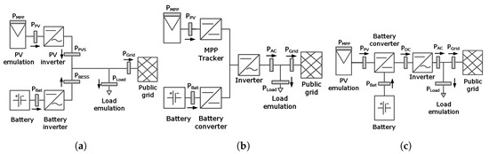
Figure 1.
Components and battery coupling of AC—(a), DC—(b), and generator (c) coupled systems indicating points of measurements in laboratory setup.
- AC-coupling: In AC-coupled systems; the battery is connected to the household installation via a bidirectional inverter (see Figure 1a), that controls the power flow of the storage system and ensures a safe and adequate battery operation. A separate PV inverter is required for connecting the PV generator and Maximum Power Point (MPP) tracking. An advantage of AC-coupling is that the PV- and the storage system may be purchased, modified, and operated independently of each other. The high number of conversion stages and associated losses which occur during charging the battery from PV is a disadvantage of this topology.
- DC-coupling: To reduce conversion losses, PV and battery use a shared inverter in DC-coupled systems (see Figure 1b). Here, the PV generator and the battery are connected on a DC link via DC/DC-converters which control the MPP tracking and the desired battery operation. With this topology losses can be significantly reduced, as no conversion to AC takes place during charging. However, increased system complexity and control requirements are disadvantages of DC-coupling.
- Generator-coupling: In generator-coupled systems, the battery is connected directly to the DC line of the PV system via a DC/DC-converter (see Figure 1c). Thus, it is charged directly by the PV generator and makes use of the PV inverter for connection to the household installation. As the battery is connected to the PV system on the DC level, this technology can be regarded as a special form of DC coupling.
In addition to fully integrated systems, which contain all the necessary elements of a PV storage system in one cabinet, single components (e.g., battery or battery inverter) for use in an individual modular system structure are widely available. As shown in [4,5], the storage capacities of residential PV battery systems are mainly between 2 kWh and 10 kWh. Furthermore, it is indicated that these capacities often correspond to the installed PV power and local energy consumption in such a way that a full cycle of the battery can be used on many days of the year.
1.2. Requirements for Performance-Assessment Methods
To be a worthwhile investment for the end-user, the high performance of PV battery systems is crucial. However, due to the diversity of system components and different technological concepts both, defining adequate performance test procedures as well as a method for the subsequent derivation of suitable key performance indicators (KPIs) are complex problems. As solar irradiance and (usually to a minor extent) power consumption of a typical household are subject to seasonal fluctuations, the battery utilization and loads on power conversions of PV battery systems vary over the year. While the battery of systems in central Europe is typically fully charged on a clear summer day, PV power rarely exceeds the local consumption on a cloudy winter day. As a result, the battery gets less utilized during the winter, and the system may often remain in standby mode. Therefore, regional and seasonal conditions must be appropriately considered in a performance evaluation. In addition to the efficient power conversion and storage, the main purpose of system deployment is to increase self-sufficiency and self-consumption. To achieve this, it is of great importance that the provided output energy follows the household’s consumption as quickly and as accurately as possible. Here, deviations between required and provided battery power result in unnecessary energy exchanges with the mains and consequently reduce self-sufficiency [6].
As the measurement results form the data basis of the KPI derivation, they must appropriately quantify all relevant influences on system performance. These influences can be classified according to their impact on efficiency or effectiveness:
- System efficiency
- -
- Operational losses due to energy conversion, MPP tracking, and energy storage
- -
- Auxiliary losses due to standby consumption and supply of external components
- System effectiveness
- -
- Power exchange with the grid due to slow or inaccurate control of output power
- -
- Power exchange with the grid or curtailments due to unfavourable energy management
Two different test categories (or a combination of both) may be applied for performance assessment [7]:
- Modular tests: Application-independent tests to separately quantify various loss mechanisms via targeted measurements of different operating states (e.g., by a separated analysis of the power flows according to Figure 2)
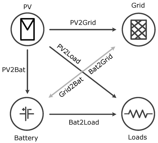 Figure 2. Power flows in PV battery systems
 - Application tests: tests that focus on system performance in multiday applications based on laboratory emulations of irradiance and load profiles
The ‘Efficiency Guideline for PV storage systems’ [8] (Efficiency Guideline), which was developed in a German joint working group of manufacturers, test facilities, and scientists defines modular test procedures for this purpose. It is based on investigations on the conversion efficiencies of the power flows of Figure 2 and contains additional measurements on storage efficiency, usable capacity, and standby consumption. Furthermore, tests to determine stationary and dynamic control deviations are proposed to quantify the influences of system control. The test procedures defined in the Efficiency Guideline have been continuously developed in recent years and are now in the process of standardization.
Several requirements also exist for the subsequent determination of KPIs. To ensure applicability for the end user, it is essential that the KPIs reflect the annual performance at the customer’s site (Requirement (R)1), are easy to understand, and that as few as possible are necessary for the system assessment (R2). Taking into account the market diversity, especially regarding the coupling of PV and battery, KPIs must be derivable for all established technologies and thus allow a comparison between systems of a different technical concept (R3). To provide results for systems that are available with (modular) expandable battery capacities, they must enable an assessment of the fundamental components and their different combinations (R4). This is also important to estimate the resulting performance when system components are replaced. Applicability or transferability to other technical solutions to increase self-sufficiency (e. g. heat pumps or electrical cars) is of great benefit, as such a feature enables a performance comparison of PV battery systems with technologies that use sector coupling (R5). As electricity and PV feed-in tariffs are subject to change and vary widely within Europe [1,9] a KPI derivation that is independent of economic considerations is beneficial to ensure validity on an international level (R6). This is also of particular importance as studies show that in Germany the decision to purchase a PV battery system is often made not only for economic reasons but also to decrease dependency on utility companies [4,5]. Finally, the KPI calculation should only require data that can be measured with a low laboratory effort and a high potential for test automation to minimize costs of performance assessment (R7).
1.3. Structure and Contributions
In the presented study, different methods for performance evaluation are examined in theory and practice. This includes a comparison of the Efficiency Guideline test procedures to application tests and a discussion concerning their benefits for KPI determination. In this way, the work contributes to the systematic elaboration of the advantages and disadvantages of both test approaches. A procedure for performance evaluation based on a KPI for (i) efficiency and (ii) effectiveness is introduced and compared to other methods such as the system performance index (SPI) [10], which is currently prevalent in Germany. The methodologies are practically applied with five different devices under test (DuT) and their advantages and drawbacks, especially focusing on peculiarities of the DuT, are identified and discussed.
This article is structured as follows. In Section 2, methodologies for system testing and KPI derivation, as well as the laboratory setup and the DuT are introduced. Section 3 presents the results of test procedure applications and KPI determinations. Essential advantages and drawbacks are analysed and evaluated within this section. The article concludes with the discussion and conclusions in Section 4.
2. Materials and Methods
2.1. Test Procedures for Performance Evaluation
Two different test approaches, namely modular tests (Section 2.1.1) and application tests (Section 2.1.2), are outlined and discussed in this section. Figure 1 indicates the positions of power measurements in a test setup that may be used with both test categories. Here, the positive counting direction of power flows is indicated by arrows. Hence, battery discharge and export of power to the grid are counted positive. To facilitate readability, all measurement setups are depicted as single-phase versions but can be implemented in a three-phase type likewise. Regardless of system topology, power flows at the following terminals are measured: PV emulation (), battery (), load emulation (), and public grid (). In addition to these, the MPP power at PV emulation () shall be logged during the tests to allow an assessment of MPP tracking.
The output power may be calculated from the sum of (PV inverter) and (battery inverter) in the case of AC-coupling or measured directly () at DC- or generator-coupled systems. The measurements enable a calculation of the energy efficiency of the entire system and its major components. Furthermore, other important parameters, such as power exchanged with the public grid and load covered by the PV battery system may be determined.
2.1.1. Modular Test Procedures
The Efficiency Guideline [8] contains various modular test procedures that have been continuously reviewed and developed over the past years. The underlying approach and configuration of the tests are briefly described in this paragraph.
Concerning the diverse system types, the power conversions of Figure 2 may consist of several steps as shown in Table 1. As power and terminal voltages are important influences on the conversion efficiency of power electronic devices [11,12,13], the conversion efficiencies need to be identified at different power levels with the terminal voltages occurring during system operation. Here, step profiles similar to IEC 61683 may be used [14]. However, the focus of IEC 61683 is on PV inverter systems, and the power at the battery terminals during typical operations of PV battery systems is different from PV inverter applications [5]. Thus further steps in partial load range may be added to the step profile. Regarding the influence of terminal voltage on conversion efficiency, the voltage dependency on the SoC has to be taken into account. Consequently, measurements on charging (PV2Bat or AC2Bat) and discharging (Bat2AC or Bat2PV) efficiency must be either performed over full battery cycles or at a well-defined SoC. Here, the Efficiency Guideline proposes measurements in a medium SoC as they are easier to represent in a generalized test procedure. In comparison to IEC 61683, the test procedures to determine conversion losses contain additional steps at 20% and 30% of the conversion path’s nominal power.

Table 1.
Conversion steps of PV battery systems depending on type of battery coupling.
Storage efficiency and capacity are tested by repeatedly charging and discharging the battery at different power levels (25%, 50%, and 100% of the nominal charge and discharge capacity). To determine dynamic control deviations the system operation is measured during several repetitions of a dynamic load profile consisting of 14 steps. Here, the steps correspond to load changes in the range of 25% to 75% of nominal discharging power and their duration is set to twice the response time identified in a preceding step response test. In the evaluation, average response times and down times are determined for charging and discharging operation. The stationary deviations are determined either from the measurement series of the conversion efficiencies (Version 1.0) or from an investigation based on the dynamic test profile (Version 2.0).
The obtained results by these test procedures are well-suited to allow for experts to assess individual key influences on system performance (such as [15]). However, the large number and complexity of the required measurements result in high expenditure of time in terms of laboratory tests and evaluations. Application-independent system evaluation may be considered via smart aggregation of the test results. However, it is unclear how the specific results can be used to derive KPIs as the guideline does not introduce an aggregation method. The tests also do not include investigations on energy management.
2.1.2. Application Test Procedures
The approach of application testing is to measure the power flows in a laboratory during realistic system operation for several days. Therefore, suitable test profiles need to be defined to reproduce the PV generation and electricity consumption applying PV and load emulations. The power flows measured during the test can be used in the next step to calculate KPIs. The resulting operating conditions and power flow on system components are highly dependent on the selected test profiles. Consequently, it is of great importance that these profiles adequately reflect fundamental daily and annual characteristics. Appendix A presents a corresponding method to derive test profiles from long-term measurement sets. For the investigations presented here, measurements from Kassel (central Germany) were applied. To enable an assessment of system effectiveness, it is essential to analyse the impacts of control speed and accuracy. Here, earlier studies have shown that sampling rates below 1 Hz can significantly reduce the PV self-consumption [6], so a temporal resolution of at least 1 s is recommended for the test profiles. To minimize test duration, effort, and associated costs, the profiles should be as short as possible. This is obviously in contradiction with a high degree of conformity to annual characteristics, so a solution must be found which satisfies both of these requirements. Another important issue is the energy content of the battery at the beginning and end of the test. Especially concerning efficiency calculations, an identical initial and final SoC needs to be defined. To increase the reproducibility, either an empty () or full battery () should be chosen here. Due to the energy demand in the evening and absence of PV power generation at night, the battery is typically empty in early morning hours. Consequently, the start and stop instants of the test profiles should be chosen to the times of sunrise and an empty battery as the initial and final state. When the annual operation of PV battery systems is reflected in the test profiles, many important influences on the system performance are directly taken into account as they occur in real operation. However, the results gained from the test only apply for the investigated system, and any change in the setup requires a new instance of the application test. For this reason, combined performance assessment with additional modular tests may be advantageous, as it could facilitate a performance estimation for use cases with consumption (or PV generation) profiles that are very different from the performed application test [7], for example, when electrical consumers for heating and air conditioning or electric cars strongly influence the electrical-load profile.
2.2. Derivation of KPI
A KPI derivation may be based on the results of both application tests and modular tests. Here three different methods are considered:
- Hybrid Benchmark: A combined assessment based on the results of application testing and modular tests with a focus on efficiency and effectiveness as proposed in [7,16,17] → Section 2.2.1
- SPI: An assessment via estimation of the economic benefit generated by the system, based on generic performance models (GPM) that are parameterized using test results of the Efficiency Guideline as proposed in [10] → Section 2.2.2
- Euro-Eta for PV battery systems: An assessment by aggregating the conversion and storage efficiencies identified in the Efficiency Guideline tests to a KPI as proposed in [18] → Section 2.2.3
Figure 3 schematically shows how laboratory measurements and simulation investigations are combined to achieve KPIs in these methods.
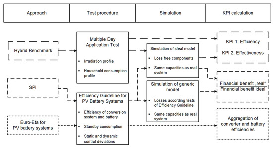
Figure 3.
Schematic overview of approaches to achieve KPIs
2.2.1. Hybrid Benchmark
The basic concept of this methodology is to determine system performance in an application test by considering one KPI for energy efficiency and one for the effectiveness of system control .
The points of measurements indicated in Figure 1 allow the calculation of important figures for performance evaluation, e.g.,:
- MPP energy provided by the PV emulation:
- PV energy generated at the DC side of the PV system:
- AC output energy of the PV battery system:
- Load covered by PV battery system:
- Energy consumed from the grid:
- Energy fed to the grid:
With these energy values, can be calculated as the ratio of output energy of the DuT to input energy provided at the PV emulation. Thus, it describes the losses that have occurred during the application test and corresponds to energy efficiency, which is a major parameter for performance evaluation:
To assess effectiveness, is determined by a combined use of laboratory measurements and simulations. Figure 4 illustrates this methodology schematically. Here, the share of local consumption covered by the PV battery system is taken into account and compared to a generic reference case. This case is characterized by an identically dimensioned but ideal system, i.e., with lossless components and idealized operating strategy as presented in Table 2. For this reason, the nominal conversion power capacities as well as the usable battery capacity are used for model parameterization. In the next step, this model is simulated with the power flows measured at the PV and load emulators during the application test. Finally, the effectiveness is calculated by comparing the load supply of the laboratory test to this simulation reference:
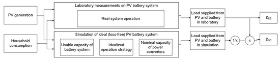
Figure 4.
Determination of and in the application test.
Table 2.
Self-consumption maximizing operation strategy.
This separate consideration of efficiency and effectiveness enables the assessment of the system performance based on two KPIs. It should be noted that a reduced efficiency directly affects the output energy provided by the system. However, in the case of sophisticated energy management, it is primarily the amount of PV power fed directly to the grid that gets reduced. Therefore a division with is not advisable for the calculation of . Nevertheless, it is desired to decouple both KPIs as much as possible. Since MPP tracking losses are already contained in , they are not in the focus of the effectiveness assessment. Consequently, the measured input power after MPP tracking is used for the system simulations.
A well-performing system must guarantee both: high energy efficiency and high effectiveness, so that both KPIs may be viewed with equal importance for most applications. For use cases that differ significantly from the application test, they can still be used, but a scaling review must be performed. Since a larger PV system leads to increased energy flows through the PV battery system, a high becomes more important in this case. In contrast, higher power consumption in the household provides increased potential for PV self-sufficiency, which makes more important. Similar considerations apply to different feed-in compensation and consumption tariffs. As long as the margin between both is low, high efficiency is of paramount importance but when consumption tariffs far exceed the feed-in compensation, high self-sufficiency and thus a good gain in importance. As the results gained from the test only apply for the investigated system, any change in the setup requires a new instance of the application test. For this reason, a combined performance assessment with additional modular tests on conversion and storage efficiency is advantageous as it also facilitates a performance estimation for use cases with a partly different setup.
2.2.2. SPI (System Performance Index)
This approach has been proposed to avoid application testing and thus provide results that are independent of test profiles and the investigated setup [19]. For this purpose, the results obtained by applying the Efficiency Guideline are used to parameterize GPMs. Here, three models for the different types of battery coupling are introduced [20,21]. In addition to the nominal conversion capacities and battery capacity, the required parameters include power-dependent conversion efficiencies, battery losses, stationary and dynamic control deviations, and standby consumption. The system operation is analysed by a simulation with PV generation and household consumption profiles [22]. As with the Hybrid Benchmark method, the simulation of an identically dimensioned ideal system is used as a reference [10]. For KPI calculation, the following values are derived following Equations (8)–(11):
- Energy consumed from the grid without PV battery system
- Energy consumed from the grid in the simulation of an ideal system
- Energy consumed from the grid in the simulation of a GPM
- Energy fed to the grid in the simulation of an ideal system
- Energy fed to the grid in the simulation of a GPM
In the next step, the resulting electricity costs C are calculated, i.e., the balance of expenditures for grid consumption and revenues for PV feed-in. Consequently, the PV feed-in compensation and electricity tariff are essential parameters for deriving . A of 12 ct/kWh and a of 28 ct/kWh are suggested for this purpose [10].
To determine , the realized cost savings of the generic performance model is divided by the cost-saving potential of an identically specified ideal system.
Following this methodology, different system combinations may be evaluated by varying model parameters. However, estimation of conversion losses during the operation of DC-coupled systems is a challenge as it is usually not possible to access the DC-link during laboratory investigations. Since the efficiency of the power conversions of Figure 2 can not be assigned to individual components here, modular measurements do not allow a loss calculation for the separate conversion steps in DC systems. Additional efficiency measurements in mixed operation modes that may serve as a remedy here [23] come along with a distinct increase of measurement effort and complexity. In addition, as application-independent testing provides no insight into energy management, specific features of system operation have to be neglected within the GPMs.
2.2.3. European Efficiency for PV Battery Systems
The concept of this approach is to evaluate system performance on the basis of an aggregation of the measurement results according to the Efficiency Guideline [24]. Here, the ‘Euro-’ for PV inverter as defined in EN 50530 [25] is used as a role model and a methodology to quantify the efficiency of the power conversions and of the battery in a single figure is pursued. Therefore, a set of scaling factors has to be defined to determine the average efficiencies of individual power conversions and storage. This may be performed either individually for each system specification or with a uniform set of scaling factors independent of nominal conversion power and storage capacity. Table 3 shows a suggested set of scaling factors and Equation (18) shows the formula proposed to calculate the aggregated efficiency of charging conversion. Analogous formulas are defined for the other operation modes.
Table 3.
Weighting factors of the Euro- approach.
Subsequently, the resulting average conversion and storage efficiencies are aggregated into a KPI. In [18], two methods are presented, each with different formulas for the types of battery coupling. In the presented work, the ’Calculation including PV’ is used:
As no scaling factors for the multiplicands are given, the share of the input energy that is not stored in the battery is neglected. Consequently, the conversion efficiency of directly used PV power is not reflected in the result. Nevertheless, the Euro- approach offers significant advantages, as it does not rely on application testing and only requires the measurement results of the conversion and storage efficiencies.
2.3. Testbench
The test bench used for practical investigations includes PV and load emulators, control computer, signal converters, and data acquisition and storage. The power flows are logged on the measuring device, while the MPP power of the PV emulator is recorded by the control computer. For PV emulation, a “PVS30000” from Spitzenberger & Spies GmbH & Co. KG [26] is used. It has a rated output power of 30 kW and a maximum output voltage of 950 V. By using an analogue series regulator at its output, the PV emulation achieves a very fast and dynamic simulation of the -characteristic [27]. The dynamic simulation of this curve is particularly important to properly emulate the system response of a PV system to the 100 Hz ripple at the DC input of the MPP tracker that is used in some tracking algorithms [28]. As load emulation, three 7 kVA AC loads of the “ZSAC” product group from Höcherl & Hackl GmbH are used [29]. Both PV and load emulation are remotely controlled using Python [30] for test automation and signal processing from the control computer. For power measurements and data recording, a “DEWE2600 all-in-one measurement instrument” from Dewetron GmbH including various high-precision zero-flux transducers and current clamps is utilised [31].
2.4. Devices Under Test
Table 4 shows the fundamental technical details of the DuT. They differ in terms of usable capacity, converter power ratings, the ratio of storage capacity to maximal charging and discharging power, and the type of battery coupling to the PV system. They cover both fully integrated concepts and setups with different degrees of modularity.
Table 4.
Major specifications of the DuT.
System A is a battery inverter that is to be used in parallel with a PV system. It can be operated with a lead-acid or a Li-ion battery that is either purchased separately or offered in a package with the inverter. For the investigations presented here, a Li-Ion battery with a usable capacity of 5.3 kWh was used [32]. Unlike System A, Systems B and C included a Li-ion battery and an associated inverter in a shared cabinet. What is remarkable about the system design of System B is the comparatively low ratio of charging power to usable battery capacity. System C has the same power ratings as those of System A while offering a considerably larger battery. Systems D and E are DC-coupled Li-ion systems that provide higher battery voltages compared to the AC-coupled DuT. With a usable capacity of only 2.2 kWh, System D offers the smallest battery, while its conversion power ratings are similar to those of System B. In contrast, System E has the largest storage capacity and highest power ratings. Since all AC-coupled systems do not include a PV inverter, an SMA Sunny Boy 5000TL [33] with a rated AC power of 4.6 kW was used to complete the laboratory setup. At the time of performing the presented measurements, the batteries of Systems A and E had already been in the laboratory for about three years. Similarly, System D had been operated in the laboratory for approximately two years before the measurements, while Systems B and C were tested in a new condition.
During preliminary investigations on the DuT, it became clear that all except System B finish the charging operation with a short constant voltage phase. The charging behaviour of System B shows an unexpected operation, in which shortly before reaching full charge, the charging power is initially reduced to −165 W and then operated for several hours with an oscillating power in the range of 30 W (discharge) to −165 W (charge) (see Figure 5). It could also be observed that this system has a threshold value for activating charging mode as a targeted charging of the battery with less than −100 W is not possible. Another important observation of the preliminary tests concerns the power control of System D. Here, different system reactions to ascending and descending step profiles are detected during both, charging and discharging operations (see Figure 6). While the system power almost instantly and completely adapts to descending steps, the response to ascending steps shows delays and the change of power flows often does not become fully compensated. As the step profiles of the Efficiency Guideline are defined with descending steps, this behaviour is not of major concern in these tests. However, the influence of the control of System D must be taken into account during performance assessment.
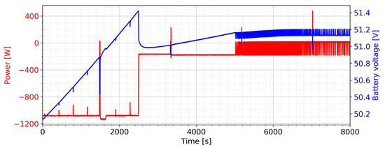
Figure 5.
Charging behaviour of System B.
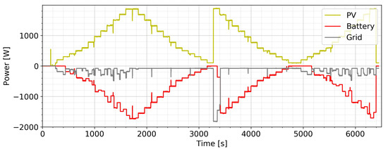
Figure 6.
Response of System D to different step profiles.
3. Results
This section presents and evaluates the results of laboratory measurements on the DuT and the subsequent determination of KPIs. It is structured as follows. First, Section 3.1 introduces the results of the investigations according to the Efficiency Guideline and highlights essential findings on system performance. In the next step, Section 3.2 examines the operation of the DuT in a 7-day application test and presents the resulting energy sums of grid feed-in, grid consumption, and load coverage. The system operation is discussed concerning peculiarities of the DuT and their influence on performance. Within Section 3.3, KPIs resulting from the laboratory measurements are determined. It includes the direct calculation of the application-dependent KPIs , , and from the measurement series of the application test, as well as the from the detected conversion and storage efficiencies. Furthermore, a determination of the from simulations applying GPMs with the time series of the application test is done to analyse resulting KPI deviations to the laboratory operation. In Section 3.4, the resulting KPIs are discussed and compared concerning their conformity to the requirements of performance assessment.
3.1. Investigations of Efficiency Guideline for PV Storage Systems
The Efficiency Guideline defines not only measurement and evaluation procedures but also associated datasheets. These summarize essential results of the investigations and also serve as uniform data sources for the parameterization of GPMs. Appendix B contains the datasheets derived for the five individual DuT. In this subsection, the results are briefly discussed.
3.1.1. Conversion Efficiencies
The investigations presented here base on separate consideration of the conversion paths shown in Figure 2 and Table 1. For reasons of clarity, the following curves depict the conversion efficiency for the relative load of the associated conversion path; i.e., the measured operating points divided by the nominal power of the conversion path (see Table 4). The corresponding absolute conversion power may vary considerably between the systems due to their different specifications.
PV2AC
Figure 7 depicts the PV2AC efficiency at nominal MPP voltage. Only one curve is plotted for Systems A, B, and C as they use the same PV inverter. The PV2AC efficiency curves of this PV inverter and System D show an efficient PV2AC operation over the entire range. Efficiencies greater than 95% are reached at the power levels above 20%. The PV2AC efficiency of System E is significantly worse, especially in the partial load range. However, it increases with the input power, achieving a similarly efficient operation in the high-power ranges.
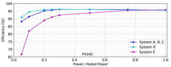
Figure 7.
PV2AC efficiency over degree of power capacity utilization.
PV2Bat
The upper part of Figure 8 shows the PV2Bat efficiency at medium SoC levels, while the bottom part depicts the AC2Bat efficiency of the AC-coupled systems. The results reveal a higher PV2Bat efficiency of the DC-coupled DuT due to their omission of a second conversion stage. System D offers the best overall efficiency and peak efficiency of 96.1% is more than 1 pp better than that of any other system. However, it has a considerably smaller PV2Bat operating range than Systems A, C, and E and prevents its battery from charging at power levels below 10% of nominal charging power. In contrast to System D, the PV2Bat efficiency of System E is weak at low power levels. The advantage of DC-coupled systems only becomes apparent at higher charging power here, where the efficiency of System E exceeds that of the AC-coupled DuT. Systems A and C have an almost identical PV2Bat efficiency. Especially in the partial load range, it is competitive or even higher than that of System E. Figure 8 reveals very high conversion losses during charging of System B. This is mainly due to its very low nominal charging power compared to the power capacity of the PV inverter. However, in contrast to Systems A and C, the AC2Bat efficiency of System B is also unsatisfactory (see Appendix B). For example, efficiency at 20% of the nominal charging power was almost 20 pp below that of other AC-coupled systems. In summary, the DC-coupled DuT, in particular System D, showed an efficient charging operation, while System B had clear weaknesses due to its comparatively inefficient AC2Bat operation.
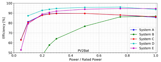
Figure 8.
PV2Bat-efficiencies over degree of power-capacity utilization.
Bat2AC
Theoretically, similar results are expected for the conversion efficiency in the discharge mode of AC- and DC-coupled systems, as both types perform comparable conversion steps. As with previous conversion efficiencies, Figure 9 shows a nearly identical curve for Systems A and C with a good efficiency in the range of 90% and above. All other DuT have a significantly higher share of losses at low power levels. The peak efficiency of System B is only 92%, while System E only shows an efficient operation in the higher power ranges. In summary, Systems A, C, and D show better Bat2AC efficiency than Systems B and E.
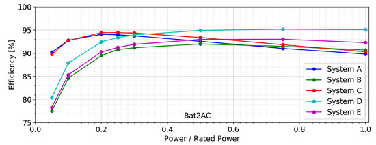
Figure 9.
Bat2AC efficiencies over degree of power capacity utilization.
3.1.2. Battery Efficiency
System D achieves the highest battery efficiency of 96.0% in the Efficiency Guideline tests. The results of Systems C and E are about 3 pp and 2 pp lower. Both the systems supply internal consumers, e.g., the display via the battery, which results in a decreased efficiency during the long test periods at low power levels.
3.1.3. Standby Consumption
While Systems A and C, supply on the DC side during standby, System D exhibits opposite behaviour as it consumes standby power only on its AC side. With only 3 W, its standby consumption is minimal. System E’s absolute standby consumption of 37 W is more than ten times higher than that of System D and almost five times higher than those of Systems A and C. System B consumes a similar standby power as System E.
3.1.4. Control Deviations
The Efficiency Guideline distinguishes between stationary and dynamic control deviations. It defines a separate test procedure for identification of dynamic properties, while stationary deviations are determined from existing investigations. In the first version of the Efficiency Guideline the step profiles of the conversion efficiencies were used for this purpose, while it is performed on the basis of the dynamic test profile in the second version. The investigations described here were based on the first version. In both cases, determination of stationary deviations is based on the average control deviations before transition to a new operating point.
Theoretically, small stationary deviations are desirable to achieve high effectiveness. However, a stationary deviation close to 0 W may quickly lead to a battery discharge into the grid (e.g., in the case of rapid load changes) and thus reduce effectiveness. While System E charges most of the residual power into the battery, Systems D and B show significantly different behaviour with resulting deviations of 79 W and 56 W. In principle, a high stationary deviation in charging mode reduces the achievable self-sufficiency by feeding excess power to the mains instead of charging the battery for later use. However, given the system design of System D with a battery capacity of only 2 kWh and a nominal Bat2AC power of 1.8 kW, a negative influence on the achievable self-sufficiency is questionable. Since System B has a much higher ratio of battery capacity to nominal Bat2AC power, these deviations can be more critical here. Taking into account the deviations during discharge operation, Systems A, B, and C show an overfeeding of the local consumption. In contrast, the negative stationary deviations of Systems D and E result in power consumption from the mains. Although this behaviour results in slightly lower instantaneous load coverage it does not necessarily reduce the system effectiveness as the energy is available to supply consumption later. Figure 10 shows the step responses of the DuT to a load step from 10% to 90% of nominal Bat2AC power. System D responds very quickly and reaches its new operating point in less than 4 s. Systems A and C respond to the load step with a of approx. 1 s and a response time of approx. 7 s. System B shows a similar behaviour but reduces its output power shortly after entering the tolerance band for the first time. More than 12 s elapse until it finally enters again. In the depicted step response, System E has the longest and shows a different behaviour since it overshoots the new set point. Similar to System D, it shows a pulsed control.
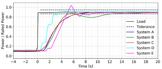
Figure 10.
Step responses to load steps from 0.1 to 0.9 of rated discharge power.
In the guideline’s dynamic test profile, except for System B, all systems achieve an average down time of less than 1.5 s and an average response time in the range of 4–7 s while System B reaches slower control parameters. In Section 2.4, the sensitivity of System D’s step response to the step direction has already been shown (see Figure 6). This behaviour also occurs during the dynamic test profile and causes difficulties in the evaluation, as it does not reach a proper system response within the step’s holding time often. If these steps are ignored in the evaluation, a down time of 1.1 s and a response time of 4.1 s are achieved. However, if these steps are evaluated with the holding time of System D’s dynamic test profile (10 s), the down time becomes 4.1 s and the response time 6.1 s.
3.2. Results of Application Tests
This section introduces power flows, energy quantities, and component efficiencies resulting from application tests with the DuT. Here, a combination of the three- and four-day test profiles determined in Appendix A to a seven-day profile is used.
Table 5 lists the energy sums at the points of measurement during the application test and the resulting component efficiencies. Since it is not possible to calculate the individual conversion efficiencies of DC-coupled systems, some of these fields remain empty. The irradiance profile at the input of the PV emulator is identical in all tests, but the simulated IV-characteristic curve is adapted to the nominal PV power of the systems. A comparison of and shows differences in the MPP tracking quality. Particularly noteworthy here is the low MPP tracking efficiency of System E (96.0%). System D shows better characteristics still, is about 1 pp below that of the AC-coupled systems here. Due to the DuT specifications, different charging energies () appear at the AC side of Systems A, B, and C. System B reaches a considerably lower battery inverter efficiency than Systems A and C, especially regarding discharge operation. Here, of Systems A and C are 6.5 pp and 8.7 pp better than that of System B. Concerning battery efficiency (), a large difference of 6.8 pp is visible between System D (96.7%) and System C (89.9%). The load profile in the application test thus leads to a significantly lower battery efficiency for System C compared to the determination according to the Efficiency Guideline. The battery efficiencies of the other DuT are relatively close to each other in the range of 93.9%–95.1%. By dividing the discharge energy () by the mean value of the DuTs’ battery capacity, the cycles of each system in the application test can be determined. Here, Systems C and E pass through a little less than four full cycles while System D almost completes six. The load coverage (), and the energy exchanges with the grid ( and ) are crucial results of the application test as they are essential inputs for KPI determinations. Theoretically, a system with a larger battery achieves a higher load coverage and thus a lower energy exchange with the grid, which becomes apparent when comparing with the battery capacities in Table 4. However, System D reaches a very high level of (13.4 kWh more than System E), but despite its much smaller battery, only decreases by 9.5 kWh compared to System E. These results also indicate much better performance in the operation of System D.
Table 5.
Results of 7-day application test with Systems A–E.
The laboratory investigations demonstrated the efficient operation of System A, and especially of System D. The other DuT showed weaknesses in several areas. In System B, this was in regard to losses of the battery inverter and system control; in System C, battery efficiency; and in System E, conversion efficiency at partial load and MPP tracking. For the final evaluation, the next section presents the resulting KPIs according to Section 2.2.
3.3. Determination of Key Performance Indicators (KPIs)
Table 6 indicates input parameters and results of the KPI calculation using measurements of the application test. The upper part shows and , the centre part contains obtained economical impacts of system operation as input for calculation, while the lower part shows conversion and storage efficiencies according to .
Table 6.
KPI calculation of application test with Systems A–E.
In terms of system efficiency, System D was the best, achieving an of 91.9%. It was followed by System A at 88.6%, System B at 86.2%, and System C at 85.6%. System E received a weaker with a result of 80.6%. System D also reached the highest within the test. In addition to high efficiency, it also shows a very effective operation, as it achieves almost the same load coverage as its lossless model. Due to good energy management, the losses occurring during operation almost exclusively result in a lower grid export with this DuT. System A achieves the second-best result in terms of effectiveness. Systems B and C, which achieve a comparable , differ more significantly in due to better dynamic behaviour and lower stationary control deviations of System C. Therefore, despite its moderately lower efficiency, System C may be preferred to System B in most cases. With an effectiveness value of 82.2%, System E achieves only a 2 pp higher than System B and thus shows the weakest performance in the application test concerning the Hybrid Benchmark KPIs. This ranking is also reflected in the . System D clearly leads with 93.6%, followed by System A with 89.1%. Systems C (85.1%), B (82.7%), and E (82.0%) achieve weaker results. It is also remarkable that is always in between the Hybrid Benchmark KPIs. The shows a different picture as the multiplication of component efficiencies leads to significantly lower results. For all systems except System E is approximately 10 pp lower than . In particular, System B achieves a low result here, as the share of PV energy which is consumed or fed to the mains without being stored in the battery is not taken into account. It can be concluded that the Hybrid Benchmark KPIs and the SPI are well applicable and allow an assessment of PV battery system performance. In the analysis presented here, both approaches provide similar results and provide the same performance ranking of the DuT.
In a final analysis GPMs developed by researchers of the University of Applied Sciences Berlin are applied and parameterized with the results of modular tests ([20,21]). For the analyses presented, models are simulated with the power flows at the PV- and load emulation during the application test. Figure 11 shows the deviations of resulting KPIs to those of the laboratory tests. While is very well satisfied with Systems A and C, System B shows a higher efficiency with a relative increase of 1.4%. This likely resulted from the charging behavior shown in Figure 5. This behaviour is not reflected in the model because it is not detected by the tests of the Efficiency Guideline (they are performed only at a medium SoC). System efficiency was about 2% higher with both DC-coupled systems, which could be due to the modelling issues of this topology. The deviations of are largest at Systems B, C, and E. Again, the battery simulation of System B leads to a too positive result here. Similarly, from System E is higher than in the laboratory application. The operation strategy of System D, which proved to be good in terms of effectiveness, is not sufficiently reflected here, so that the system reached a result that was approx. 4% too low comparing to Systems B and E. Here, critical factors are missing in the calculation of KPIs due to the lack of modelling operation strategy. The SPI deviations are consistent with these findings and are approximately equal to those of the efficiency parameter.
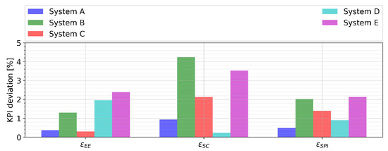
Figure 11.
Deviation of KPIs between simulation and laboratory measurement.
3.4. Evaluation of Performance-Assessment Methodologies
Reconsidering the requirements from Section 1.2, the Hybrid Benchmark method yields two KPIs that are easy to explain and simple (R2). They directly reflect a typical operation by choosing an application test as the core of performance evaluation (R1). As it requires a discharged battery at the end of the experiment, fundamental limitations exist for the storage capacity. However, in the range of reasonable system sizing, this limitation is avoided by the test profiles, so that the method proves applicability (R3). As both KPIs assess the performance of an entire system, the component efficiencies in the application test may serve to evaluate its components (R4). However, a thorough evaluation of different system combinations requires an individual application test with different setups. Considering transferability, application testing requires profiles for all household- and PV system terminals. E.g., to assess a sector coupling via heat pumps and thermal storage, an additional test profile representing heat demand would be essential. Investigations regarding this have shown the possibility to evaluate complex PV–CHP systems through application testing [33], and the focus on efficiency and effectiveness is very well-suited to assess different system setups (R5). The method does not relate to any country-specific tariffs. However, selecting test profiles requires a broader international perspective (R6). Compared to extensive testing effort associated with the Efficiency Guideline procedures, application tests require a fraction of time for testing and evaluation and a high potential for full automation (R7).
and prove to be advantageous in terms of the amount of KPIs and possibilities to assess different system combinations. Nevertheless, concerning international validity, the consideration of feed-in compensations and consumption tariffs within is disadvantageous. The very good conformance to R2 comes with the price of noncompliance to R6. Another disadvantage of the SPI is the effort needed for testing and evaluation. Although the use of GPMs leads to full conformance with Requirement R4, this is at the expense of a high workload in KPI determination. Here, the measurement effort associated with the Efficiency Guideline, and the subsequent parameterization and simulation of GPMs are particularly significant. Considering , its results do not reflect all aspects of system performance as it neglects important influences and bases on many simplifications. These also result in a changed order in which system E performs better than systems B and C. From the findings of the other two evaluation methods, however, this order does not correspond to the actual system performance. With both the SPI and the , the full conformance to individual requirements leads to noncompliance elsewhere, while the Hybrid Benchmark approach takes all requirements into account. These findings are summarized in Table 7, where a rating is given in terms of four result classes: (++) full compliance, (+) good compliance, (0) moderate compliance, and (−) noncompliance.
Table 7.
Compliance with requirements of applied assessment methods.
4. Discussion and Conclusions
To increase the satisfaction of PV battery system end users, a uniform methodology for comparing system performance irrespective of system topology is necessary. Core conflicts in performance evaluation exist primarily concerning the required test procedures and the method applied to determine KPIs. Here, application tests that intend to shorten the evaluation period to a few days are always associated with a specific loss of representativeness of annual characteristics. They are opposed by the use of GPMs, as these allow a systematic evaluation of various use cases by modifying simulation profiles. However, such a method requires parameters and models that accurately describe all essential operational characteristics. A targeted application of GPMs, therefore, requires a sufficient simulation of the operating behaviour and thus needs measurement procedures that go beyond the current status of the Efficiency Guideline. Although, a purely simulative determination of application-oriented KPIs is promising concerning an evaluation of different system combinations. Application-independent KPIs like the are not capable of adequately representing all essential aspects of system performance as they do not include crucial parameters like standby operation and system control. Evaluation based on KPIs for efficiency and effectiveness in application tests is advantageous here.
Concerning the performance of the DuT in this work, the DC-coupled topology shows a broad spectrum of system quality. It became clear that different characteristics of both full systems and components are fundamental for system performance. Particularly relevant are high conversion efficiency in the partial load range, an effective operating strategy with consistent avoidance of power flows between the battery and the grid as well as a storage system that is compact in terms of capacity and conversion power. Nevertheless, an efficient MPP tracking and conversion of PV power prove essential for a well-performing system. Especially regarding the operating behaviour of DC and generator-coupled battery systems, appropriate consideration of these aspects in the comparative system evaluation is crucial.
In recent years, PV battery systems also gained importance outside of Germany. As a consequence, KPIs need to be usable and valid on an international level. Thus, a review of the test profiles of the Hybrid Benchmark method under international aspects will become necessary, and an extension of test duration is likely to be inevitable. Other developments concern the increasing system complexity resulting from links of residential electricity supply to heating and climatization as well as from the aggregated operation of distributed storage systems to provide grid services. They shift the use cases from the maximization of local self-sufficiency to applications with mixed objectives. As a consequence, the evaluation of effectiveness in multiple use cases may probably gain importance in the future.
Author Contributions
Conceptualization, F.N. and M.B.; Formal analysis, M.B.; Investigation, F.N.; Methodology, F.N.; Supervision, M.B.; Visualization, F.N.; Writing—original draft, F.N.; Writing—review and editing, F.N. and M.B. All authors have read and agreed to the published version of the manuscript.
Funding
This research was partly funded by the German Federal Ministry for Economic Affairs and Energy (BMWi), grant number 03TNK015A.
Conflicts of Interest
The authors declare no conflict of interest. The funders had no role in the design of the study; in the collection, analyses, or interpretation of data; in the writing of the manuscript, or in the decision to publish the results.
Abbreviations
The following abbreviations, variables, and indices are used in this manuscript:
| AC | Alternating current or AC-coupled |
| AC2Bat | Charge operation (AC-coupled) |
| Aut | Self-sufficiency |
| Bat | Battery or DC point of BESS |
| Bat2AC | Discharge operation (AC-coupled, DC-coupled) |
| Bat2PV | Discharge operation (generator-coupled) |
| BESS | AC point of battery-energy storage system |
| c | Energy costs per [] |
| C | Capacity in [] or costs in [] |
| Battery capacity [] | |
| Charge | Charging of battery |
| CHP | Combined heat power |
| Con | Self-consumption |
| Household consumption | |
| D | Normalized deviation |
| Day | All values of the day |
| DC | Direct current or DC-coupled |
| Discharge | Discharging of battery |
| DuT | Device under test |
| EE | Energy efficiency |
| Efficiency Guideline | Efficiency Guideline for PV storage systems |
| Euro | Value of |
| Performance indicator | |
| f | Scaling factor |
| Energy costs for PV feed-in | |
| Gen | Generator-coupled |
| GPM | Generic performance model |
| Grid | Point of grid connection |
| GridEx | Export to grid |
| GridIm | Import from grid |
| Ideal | Simulation of ideal system |
| Irr | Solar irradiance |
| KPI | Key Performance Indicator |
| Lab | Laboratory test |
| Li-Ion | Lithium-ion |
| Load | Household consumption |
| LoadCvr | Load covered by PV battery system |
| Loss | Energy losses |
| MPP | Maximum Power Point |
| nom | Nominal (rated) value |
| OP | Operation Parameter |
| PP | Profile Parameter |
| pp | percentage points |
| PV | Photovoltaic |
| PVS | AC-side of PV system |
| PV2AC | Direct PV use operation |
| PV2Bat | Charge operation (DC-coupled, Generator-coupled) |
| R | Requirement |
| Ref | Household without PV battery system |
| SC | System Control |
| SoC | State of Charge |
| SPI | System Performance Index |
| Downtime [s] | |
| Response time [s] | |
| Tx | Energy per hour [] |
| X | Power fluctuation |
| Xmax | Maximum value of X |
| Xmean | Mean value of X |
| Xmin | Minimum value of X |
Appendix A. Derivation of Test Profiles for Application Tests
The objective of the work presented in this appendix is to define and apply a methodology to derive test profiles for application tests of PV battery systems.
Appendix A.1. Background
Concerning test profiles for residential energy systems, in Germany, VDI 4655 guideline is often applied [34]. It proposes reference load profiles based on typical days for testing purposes of Combined Heat Power (CHP) plants. These include electricity in 60 s resolution as well as space heating and hot water demand in 15 min resolution. The data-sets have been obtained from various long-term measurement series in single-family and multi-family houses. However, VDI 4655 does not contain any irradiance or PV generation profiles. Existing meteorological reference profiles (e.g., [35] and [36]), which could be used instead, generally process annual data in a resolution of minutes or longer periods. Considering the requirements of the application test, the low temporal resolution of these profiles is not suitable for the problem at hand. Different methods may be used to interpolate between the samples, or stochastic signals could be added to the original signal to obtain high-resolution profiles. Such approaches are discussed in various publications (e.g., [37]). Another possibility is the synthetic generation of test profiles using profile generators. Concerning electricity consumption, these often use measurements of individual electrical consumers. Through a combination with simulated usage habits of different electrical appliances in individual household types, a differentiation between various user groups is enabled [38,39,40]. For the investigations presented in this paper, a method focussing on a systematic choice and combination of daily profiles from high-resolution long-term measurements is pursued. With means of these test profiles, important statistical characteristics of the input data must be maintained [41]. A couple of publications on this topic, especially concerning grid stability issues and for models focusing on optimum electrical capacity investment, are available [42,43]. A work of particular interest for the present task is documented in [44]. This publication indicates the minimum combinatorial order to preserve annual characteristics. Although the focus is on investment planning of energy capacities, nevertheless it gives important clues for the problem at hand. A central finding is that a single annual load profile in 1 h resolution (i.e., 8760 values) can be aggregated in the order of 10 representative hours (scenario robust). However, when an additional source of variability needs to be considered (e.g., solar irradiance), the required hours of a robust aggregation increase up to an order of 1000. As a remedy, the second step of the methodology introduced here is performed on the basis of residual profiles.
Appendix A.2. Database
A central specification for the test profiles is to represent the conditions of typical applications of PV battery systems. Many systems are applied in Germany, long-term local measurements of PV power generation (resp. solar irradiance), and consumption of a typical German household served as database here. Due to its central location and availability of high-resolution measurement data, long-term measurements of the Kassel region were used. However, the methodologies described in this chapter may also be applied to other datasets. The irradiance data used here were obtained by long-term measurements in 1 s resolution on the rooftop of the Fraunhofer IEE building in Kassel, Germany. Irradiance was detected by a south-facing sensor inclined by 30°. Additionally, module temperature was recorded. The data used here refer to the period from September 2012 to August 2013. The measured irradiance during the indicated period amounted to 1109.2 , which approximately met the long-term average in Germany (i.e., 1180 [45], which corresponds to 1050 on a horizontal surface, and an annual yield increase of 12% due to the inclination and orientation of the module [46]). The electricity-consumption profiles were provided by a three-phase measurement dataset in 1 s resolution of a four-person household in the Kassel region. It was recorded from June 2010 to April 2011 and lacks data for May to complete a full year. Annual electricity consumption extrapolated from the measurement period amounted to 3540 kWh, which is between the typical consumption indicated for 4-person households (4750 kWh), but above the annual electricity consumption of an average household (3100 kWh) in Germany [47]. The long-term simulation used for the presented investigations is mapping the annual datasets to a reduced period, which is necessary as the consumption dataset does not cover a full year.
Appendix A.3. First Step—Profile Analysis
First, datasets were fragmented into daily subsets. These were analyzed to identify single subsets and combinations of these subsets that were capable of representing all data in terms of seven profile parameters (PP) (see Figure A1). Here, and correspond to the temporal boundaries of each daily subset.
- Daily solar energy and daily load demand (see Figure A1a)).
- Maximum and minimum power: , and (see Figure A1a))
- The average fluctuations , and maximum fluctuations, , and by using a low-pass filtering with a ten-minute moving average (see Figure A1b)).
- Energy per hour: and
- Energy per power level: and
Additionally, the annual averages of these parameters (e. g. and ) are calculated.

Figure A1.
Simplified general presentation of the profile parameters with daily energy, maximum and minimum power (a), upper left), average and maximum fluctuations (b), upper right), share of energy per hour (c), lower left) and share of energy per power level (d), lower right).
Figure A1.
Simplified general presentation of the profile parameters with daily energy, maximum and minimum power (a), upper left), average and maximum fluctuations (b), upper right), share of energy per hour (c), lower left) and share of energy per power level (d), lower right).

To assess how well each subset represents annual averages, the normalized deviation is defined. It is calculated separately for irradiance and load. As the applied formula is identical for both, only the irradiance variables are shown here.
The factors (, , ...) in Equation (A1) are scaling factors. They are derived by an analytical hierarchy process, where the importance of all individual PP was compared and assessed. The resulting factors are shown in Table A1. Equation (A1) may be explored to identify the best fitting daily subsets. Next, the period under investigation is expanded from daily subsets to combinations of daily subsets, which are systematically selected from the entire datasets. While advancing from daily subsets (combinatorial order of one) to subsets containing tuples of daily curves (combinatorial order of two) and higher combinatorial orders, the profile length increases. Consequently, the time instants and integral boundaries are adjusted according to the (in general) non-continuous time intervals of the subsets under investigation. These adjusted PP functions are then used to calculate the deviations for each combinatorial order.
Table A1.
Scaling factors for the first step of profile selection.
Table A1.
Scaling factors for the first step of profile selection.
| Type | Factor | |||||||
|---|---|---|---|---|---|---|---|---|
| ∑ | ||||||||
| Irradiance | 0.40 | 0.12 | 0 | 0.21 | 0.03 | 0.14 | 0.09 | 1.0 |
| Load | 0.35 | 0.08 | 0.05 | 0.2 | 0.02 | 0.15 | 0.15 | 1.0 |
Figure A2 shows the derived results, limited to the top-100 subsets. It can be seen that the deviations fall into discrete intervals for each combinatorial order: Obviously, the attempt to reflect annual characteristics using single day curves leads to a wide-spread deviation interval with the median being located at approx. 0.43 units for irradiance and 0.23 units for the load. Increasing the combinatorial order from one to two reduces the median value to 0.12 units for irradiance and 0.11 units for the load while the box sizes become considerably smaller. With a further increase of the combinatorial order up to four and five, median values below 0.05 units are achieved for both irradiance and load. It can be seen that the convergence proceeds monotonously. For any combinatorial order of 2-5, the three subsets with the lowest deviations are used for further investigation in the second step. Since different combinations of the irradiance and load candidates with the same combinatorial order are possible, the final result of the first step is a total of 36 combined profiles. These sets are called candidate profiles.

Figure A2.
Deviations from annual averages of the best 100 irradiance (a) and load (b) curves with different combinatorial order. The upper right parts show a zoom of the results for the duration of 3, 4, and 5 days.
Figure A2.
Deviations from annual averages of the best 100 irradiance (a) and load (b) curves with different combinatorial order. The upper right parts show a zoom of the results for the duration of 3, 4, and 5 days.

Appendix A.4. Second Step—PV Battery-System Operation Analysis
In the second step, the operation of PV battery systems with the candidate profiles is investigated utilizing simulations. For this purpose, a generic performance model (GPM) that is based on comprehensive modes of operation is applied and parameterized with different system configurations. The model is based on an idealized operational strategy and phenomenological equations to represent intrinsic losses. The resulting power flows are used to calculate the Operation Parameters (OP): self-sufficiency , self-consumption , and conversion losses .
The OP resulting from simulations with the candidate profiles are compared with those derived from annual simulations ( and , ). Their difference provides another set of convergence criteria expressed by the deviation function of the second step:
The second step ensures that the test profiles do not only correspond to the PPs from Appendix A.3 but also to the typical annual operation of PV battery systems. Each of the 36 candidate profiles resulting from the first step results in a set of OPs and deviations according to Equation A2. The ranges thereof are shown in Figure A3 for the five system specifications examined in Table A2. Here, OP ranges are depicted by coloured dots for the candidate profiles, while related results based on an annual simulation are indicated by black dots. Thus, a deviation of OP can be identified by comparing the position of coloured and black dots.

Figure A3.
Results of simulations with candidate profiles: self-sufficiency (a), self-consumption (b), conversion losses (c).
Figure A3.
Results of simulations with candidate profiles: self-sufficiency (a), self-consumption (b), conversion losses (c).

Table A2.
Specifications of PV battery systems used for profile evaluations with the reference model.
Table A2.
Specifications of PV battery systems used for profile evaluations with the reference model.
| Parameter | Reference System | ||||
|---|---|---|---|---|---|
| I | II | III | IV | V | |
| [kWh] | 2 | 2 | 5 | 5 | 8 |
| [kW] | 2 | 5 | 5 | 8 | 8 |
| [kW] | 2 | 2 | 5 | 5 | 8 |
| [kW] | 2 | 2 | 5 | 5 | 8 |
It can be seen that the OP of the annual simulation tends to be in the centre of areas in which the simulation results with the candidate profiles accumulate. This applies in particular to the medium-sized systems III and IV. In general, the relative losses show the least deviations of the parameters investigated. The two best profile combinations in a combinatorial order of three and four are selected for laboratory tests and further investigations. These profiles are shown in Figure A4. Both irradiance profiles use an identical first day, which indicates particularly high representativeness of this specific curve for the entire dataset.
An essential step for future investigations is to apply the presented methodology to a broader set of annual measurement data to increase the validity of the obtained profiles. Furthermore, it may be used to derive load profiles for significantly different use-cases like households with heat pumps or electric cars.

Figure A4.
Selected test profiles, three-day irradiance (a), three-day load (b), four-day irradiance (c) and four-day load (d).
Figure A4.
Selected test profiles, three-day irradiance (a), three-day load (b), four-day irradiance (c) and four-day load (d).

Appendix B. Datasheets of Devices under Test

Figure A5.
Datasheet of System A.
Figure A5.
Datasheet of System A.


Figure A6.
Datasheet of System B.
Figure A6.
Datasheet of System B.


Figure A7.
Datasheet of System C.
Figure A7.
Datasheet of System C.


Figure A8.
Datasheet of System D.
Figure A8.
Datasheet of System D.


Figure A9.
Datasheet of System E.
Figure A9.
Datasheet of System E.

References
- Stetz, T.; von Appen, J.; Niedermeyer, F.; Scheibner, G.; Sikora, R.; Braun, M. Twilight of the grids. IEEE Power Energy Mag. 2015, 13, 50–61. [Google Scholar] [CrossRef]
- Curry, C. Lithium—Ion battery costs and market. Bloom. New Energy Financ. 2017. Available online: https://about.bnef.com/blog/global-storage-market-double-six-times-2030/ (accessed on 21 April 2020).
- Figgener, J.; Stenzel, P.; Kairies, K.P.; Linßen, J.; Haberschusz, D.; Wessels, O.; Angenendt, G.; Robinius, M.; Stolten, D.; Sauer, D.U. The development of stationary battery storage systems in Germany—A market review. J. Energy Storage 2020, 29. [Google Scholar] [CrossRef]
- Kairies, K.P.; Figgener, J.; Haberschusz, D.; Wessels, O.; Tepe, B.; Sauer, D.U. Market and technology development of PV home storage systems in Germany. J. Energy Storage 2019, 23, 416–424. [Google Scholar] [CrossRef]
- Figgener, J.; Haberschusz, D.; Kairies, K.P.; Wessels, O.; Tepe, B.; Sauer, D.U. Wissenschaftliches Mess- und Evaluierungsprogramm Solarstromspeicher 3.0—Jahresbericht 2018; Institute for Power Electronics and Electrical Drives, RWTH Aachen University: Aachen, Germany, 2018; Available online: http://www.speichermonitoring.de/fileadmin/user_upload/Speichermonitoring_Jahresbericht_2018_ISEA_RWTH_Aachen.pdf (accessed on 12 June 2020).
- Braun, M.; Büdenbender, K.; Landau, M.; Sauer, D.U.; Magnor, D.; Schmiegel, A. Charakterisierung von netzgekoppelten PV-Batterie-Systemen—Verfahren zur Bestimmung der Performance. In Proceedings of the 25th Symposium Photovoltaische Solarenergie, Bad Staffelstein, Germany, 3–5 March 2010; Available online: https://www.researchgate.net/publication/216574952_Charakterisierung_von_netzgekoppelten_PV-Batterie-Systemen_-_Verfahren_zur_vereinfachten_Bestimmung_der_Performance (accessed on 28 September 2020).
- Niedermeyer, F.; von Appen, J.; Braun, M.; Schmiegel, A.; Kreutzer, N.; Reischl, A.; Scheuerle, W. Allgemeine Performanceindikatoren für PV-Speichersysteme. In Proceedings of the 29th Symposium Photovoltaische Solarenergie, Bad Staffelstein, Germany, 12–14 March 2014. [Google Scholar]
- Efficiency Guideline for PV Storage Systems, Version 2.0; BVES Bundesverband Energiespeicher, BSW Bundesverband Solarwirtschaft. Available online: https://www.bves.de/wp-content/uploads/2019/07/EfficiencyGuideline_PV-Storage_2.0_EN.pdf (accessed on 9 June 2020).
- Electricity Prices for Household Consumers—Bi-Annual Data (from 2007 Onwards); European Commission. Eurostat: Luxembourg. Available online: http://appsso.eurostat.ec.europa.eu/nui/show.do?dataset=nrg_pc_204 (accessed on 6 June 2020).
- Weniger, J.; Tjaden, T.; Quaschning, V. Vergleich Verschiedener Kennzahlen zur Bewertung der Energetischen Performance von PV-Batteriesystemen. In Proceedings of the 32nd Symposium Photovoltaische Solarenergie, Bad Staffelstein, Germany, 8–10 March 2017; Available online: https://pvspeicher.htw-berlin.de/wp-content/uploads/2017/03/WENIGER-2017_03-Vergleich-verschiedener-Kennzahlen-zur-Bewertung-der-energetischen-Performance-von-PV-Batteriesystemen.pdf (accessed on 28 September 2020).
- Mohan, N.; Undeland, T.; Robbins, W. Power Electronics: Converters, Applications, and Design; Wiley: Hoboken, NJ, USA, 2002; Volume 3, ISBN 978-047-122-6932. [Google Scholar]
- Häberlin, H. Wirkungsgrade von Photovoltaik-Wechselrichtern. ET Elektrotechnik Aarau 2005, 56, 53–57. Available online: http://www.pvtest.ch/Dokumente/Publikationen/101_etatot_ET_02.pdf (accessed on 28 September 2020).
- Mertens, K. Photovoltaics: Fundamentals, Technology and Practice; Wiley: Hoboken, NJ, USA, 2014; Volume 1, ISBN 978-111-863-4165. [Google Scholar]
- IEC 61683:1999. Photovoltaic Systems—Power Conditioners—Procedure for Measuring Efficiency; International Standard, IEC—International Electrotechnical Commission: Geneva, Switzerland, 1999. [Google Scholar]
- Munzke, N.; Schwarz, B.; Hiller, M. Intelligent control of household Li-ion battery storage systems. Energy Procedia 2018, 155. [Google Scholar] [CrossRef]
- Niedermeyer, F.; Appen, J.V.; Braun, M.; Schmiegel, A.; Rothert, M.; Kreutzer, N. Vergleich der Performance von PV-Batteriesystemen. PV Mag. 2014, 11/14, 81–84. [Google Scholar]
- Niedermeyer, F.; von Appen, J.; Kneiske, T.; Braun, M.; Schmiegel, A.; Kreutzer, N. Innovative Performancetests für PV-Speichersysteme zur Erhöhung der Autarkie und des Eigenverbrauchs. In Proceedings of the 30th Symposium Photovoltaische Solarenergie, Bad Staffelstein, Germany, 4–6 March 2015. [Google Scholar]
- Loges, H.; Rothert, M.; Engel, B. Effizienzvergleich von PV-Speicher-Systemen. EW Magazin für die Energiewirtschaft 2017, 10/17, 42–46. [Google Scholar]
- Weniger, J.; Tjaden, T.; Bergner, J.; Quaschning, V. Emerging Performance Issues of Photovoltaic Battery Systems. In Proceedings of the 32nd European Photovoltaic Solar Energy Conference and Exhibition, Munich, Germany, 20–24 June 2016. [Google Scholar]
- Tjaden, T.; Weniger, J.; Messner, C.; Knoop, M.; Littwin, M.; Kairies, K.P.; Haberschusz, D.; Loges, H.; Quaschning, V. Offenes Simulationsmodell für netzgekoppelte PV-Batteriesysteme. In Proceedings of the 32nd Symposium Photovoltaische Solarenergie, Bad Staffelstein, Germany, 8–10 March 2017. [Google Scholar]
- Maier, S.; Weniger, J.; Böhme, N.; Quaschning, V. Simulationsbasierte Effizienzanalyse von PV-Speichersystemen. In Proceedings of the 34th Symposium Photovoltaische Solarenergie, Bad Staffelstein, Germany, 19–21 March 2019. [Google Scholar]
- Tjaden, T.; Weniger, J.; Bergner, J.; Quaschning, V. Repräsentative Elektrische Lastprofile für WOHNGEBäude in Deutschland auf 1-sekündiger Datenbasis. 2015. Available online: https://pvspeicher.htw-berlin.de/wp-content/uploads/Repräsentative-elektrische-Lastprofile-für-Wohngebäude-in-Deutschland-auf-1-sekündiger-Datenbasis.pdf (accessed on 17 June 2020).
- Despeghel, J.; Tant, J.; Driesen, J. Loss Model for Improved Efficiency Characterization of DC Coupled PV-Battery System Converters. 2019. Available online: https://ieeexplore.ieee.org/stamp/stamp.jsp?tp=&arnumber=8927644 (accessed on 17 June 2020).
- Loges, H. Entwicklung einer Energieeffizienzkennzahl für PV-Batteriespeicher. Ph.D. Thesis, Technical University of Braunschweig, Braunschweig, Germany, 2019. [Google Scholar]
- CENELEC - EN 50530:2013. Overall Efficiency of Grid Connected Photovoltaic Inverters; European Standard; CENELEC: Brussels, Belgium, 2010. [Google Scholar]
- Spitzenberger und Spies GmbH und Co. KG. Photovoltaik Simulator–PVS Serie–PVS 1000/LV—Datasheet. Available online: https://www.spitzenberger.de/weblink/1064 (accessed on 22 April 2020).
- Ram, J.P.; Manghani, H.; Pillai, D.S.; Babu, T.S.; Miyatake, M.; Rajasekar, N. Analysis on solar PV emulators: A review. Renew. Sustain. Energy Rev. 2018, 81, 149–160. [Google Scholar] [CrossRef]
- Hohm, D.; Ropp, M. Comparative study of maximum power point tracking algorithms using an experimental, programmable, maximum power point tracking test bed. In Proceedings of the 28th IEEE Photovoltaic Specialists Conference, Anchorage, AK, USA, 15–22 September 2000. [Google Scholar]
- Höcherl und Hackl GmbH. Electronic Load Series ZSAC—Operating Manual. Available online: https://www.schulz-electronic.de/fileadmin/media/ZSAC_SW_B_D-E.pdf (accessed on 22 April 2020).
- Python Software Foundation. Python Language Reference; Version 3.7.4; Python Software Foundation: Wilmington, DE, USA, 2019. [Google Scholar]
- Dewetron GmbH. DEWE 2600—Technical Reference Manual. Available online: https://www.johnmorrisgroup.com/Content/Attachments/122350/DEWE-2600_manual.pdf (accessed on 22 April 2020).
- IBC Solar AG. IBC SolStore 6.5 Li—Datasheet; IBC Solar AG.: Bad Staffelstein, Germany, 2014. [Google Scholar]
- SMA Solar Technology AG. PV inverter—Sunny Boy 3000TL/ 4000TL/ 5000TL—Datasheet; SMA Solar Technology AG.: Niestetal, Germany. Available online: http://files.sma.de/dl/15330/SB30-50TL-21-BE-en-11.pdf (accessed on 23 April 2020).
- VDI-Fachbereich Energietechnik. VDI-Fachbereich Energietechnik. VDI 4655:2008—Reference load profiles of single-family and multi-family houses for the use of CHP systems. In German Technical Guideline; VDI—Verein Deutscher Ingenieure: Berlin, Germany, 2008. [Google Scholar]
- Deutscher Wetterdienst (DWD) and Federal Institute for Research on Building, Urban Affairs and Spatial Development (BBSR). Handbuch—Ortsgenaue Testreferenzjahre von Deutschland für mittlere und extreme Witterungsverhältnisse; DWD: Offenbach, Germany, 2017. [Google Scholar]
- Remund, J.; Müller, S.C. Meteodaten für die Eigenverbrauchsberechnung. In Proceedings of the 32nd Symposium Photovoltaische Solarenergie, Bad Staffelstein, Germany, 8–10 March 2017. [Google Scholar]
- Stetz, T.; Marten, F.; Braun, M. Improved Low Voltage Grid-Integration of Photovoltaic Systems. IEEE Trans. Sustain. Energy 2013, 4, 534–542. [Google Scholar] [CrossRef]
- Von Appen, J.; Haack, J.; Braun, M. Erzeugung zeitlich hochaufgelöster Stromlastprofile für verschiedene Haushaltstypen. IEEE Power Energy Stud. Summit Stuttg. 2014. Available online: https://docplayer.org/72035549-Erzeugung-zeitlich-hochaufgeloester-stromlastprofile-fuer-verschiedene-haushaltstypen.html (accessed on 23 April 2020).
- Reese, C.; Hofmann, L. Synthetic three-phase load profiles. In Proceedings of the 22nd International Conference and Exhibition on Electricity Distribution (CIRED 2013), Stockholm, Sweden, 10–13 June 2013. [Google Scholar]
- Pflugradt, N. Modellierung von Wasser und Energieverbräuchen in Haushalten. Ph.D. Thesis, Chemnitz University of Technology, Chemnitz, Germany, 2016. [Google Scholar]
- Henze, J.; Kneiske, T.; Braun, M.; Sick, B. Identifying Representative Load Time Series for Load Flow Calculations. In Data Analytics for Renewable Energy Integration: Informing the Generation and Distribution of Renewable Energy; Springer: Berlin/Heidelberg, Germany, 2017; pp. 88–93. [Google Scholar]
- Green, R.; Stafell, I.; Vasilakos, N. Divide and Conquer? k-Means Clustering of Demand Data Allows Rapid and Accurate Simulations of the British Electricity System. IEEE Trans. Eng. Manag. 2014, 61, 251–260. [Google Scholar] [CrossRef]
- Poncelet, K.; Höschle, H.; Delarue, E.; Virag, A.; D’Haesseleer, W. Selecting Representative Days for Capturing the Implications of Integrating Intermittent Renewables in Generation Expansion Planning Problems. IEEE Trans. Power Syst. 2017, 32, 1936–1948. [Google Scholar] [CrossRef]
- Merrick, J.H. On representation of temporal variability in electricity capacity planning model. Energy Econ. 2016, 59, 261–274. [Google Scholar] [CrossRef]
- Deutscher Wetterdienst (DWD). Jahresgang der Globalstrahlung 2018 im Vergleich zum langjährigen Mittel 1981–2010; DWD: Offenbach, Germany, 2018. [Google Scholar]
- Quaschning, V. Regenerative Energiesysteme; Carl Hanser Verlag: Munich, Germany, 2015; Volume 9, pp. 80–81. ISBN 978-3-446-44267-2. [Google Scholar]
- Bundesverband der Energie- und Wasserwirtschaft (BDEW) e.V. Energie-Info: Stromverbrauch im Haushalt; BDEW: Berlin, Germany, 2013. [Google Scholar]


Publisher’s Note: MDPI stays neutral with regard to jurisdictional claims in published maps and institutional affiliations. |
© 2020 by the authors. Licensee MDPI, Basel, Switzerland. This article is an open access article distributed under the terms and conditions of the Creative Commons Attribution (CC BY) license (http://creativecommons.org/licenses/by/4.0/).