Hydroelectric Operation Optimization and Unexpected Spillage Indications

Abstract

It is widely known that hydroelectric power plants benefit from optimized operation schedules, since the latter prevent water and, therefore, monetary wastes, contributing to significant environmental and economic gains. The level of detail on the representation of such systems is related to how far ahead the planning horizon is extended. Aiming at the very short-term optimization of hydroelectric power plants, which usually requires the most detailed models, this paper addresses an undesired effect that, despite being already mentioned in the literature, has not been properly explored and explained yet. This effect is given by the indication of spillage by the optimizer, even when the reservoir does not reach its maximum capacity. Simulations implemented in Julia language using real power plant data expose this phenomenon. Possible ways to circumvent it are presented. Results showed that, in specific cases, spillage allows the achieving of more efficient operating points by reducing the gross head and increasing the amount of water that flows through turbines. Furthermore, it was verified that applying water outflow-based objective functions prevents undesired spillage indications, despite causing machines to operate at lower efficiency levels, compared with the utilization of power losses-based objective functions.

1. Introduction

Optimizing the short-term operation of power plants comes down to determining which generating units (GUs) must be online, and how much power each of them has to generate while meeting all system constraints. Regardless of the system being hydraulic, thermal, hydro-thermal, or even incorporating alternative energy sources in its formulation, optimal operation schedules contribute to economic and environmental gains, i.e., they help secure sustainable scenarios concerning energy supply. In Brazil, there are multiple possible planning horizons. The widest is the long-term operation planning, which takes several years into account. The narrowest is a very short-term one, in which only the day-ahead operation is considered. The former usually includes several energy sources simultaneously and does not implement detailed characteristics of these sources. As losses of accuracy cause an immediate decrease in performance, the day-ahead operation requires high levels of detail, as in [1,2,3,4,5,6,7,8,9,10,11]. These papers consider several hydroelectric operation aspects, such as head dependency when calculating efficiency, reservoir and downstream basin levels variation, and penstock power losses. Within this context, several papers exposing researches on the very short-term operation of hydroelectric power plants (HPPs) consider spillage as a decision variable, as in [1,2,3,4,5,6,7,8,9,10,11]. In these works, determining how much reservoir water should be spilled (if any) becomes part of the optimization problem. The adequacy of such approach relies on the fact that it allows the optimizer to indicate which spillage values will keep the reservoir below or at its maximum capacity. It is important to highlight that spillage refers to water release decisions taken by operators so that excessive reservoir water can be directly sent from the upstream to the downstream basin, hence preventing the former from reaching unsafe levels.

Although the length of long-term planning (LTP) differs depending on the country, its range is usually from one to ten years. The optimization of these models typically applies stochastic methods, due to how distant in time the problem is extended [12]. Moreover, the fact that LTP considers systems with a large number of power generation facilities also adds uncertainties. Ideally, LTP would be capable of incorporating every mathematical aspect of the power plants included in the system, thus granting higher accuracy in results. However, the complexity and computational burden of such an approach require tools that are beyond today’s technology. Simplifications are done to address this issue. For instance, HPPs do not have their GUs optimized separately. In fact, the whole HPP’s power output is considered. As stated in [13], current LTP challenges relate to spinning reserve requirements and dealing with the “uncertainty regarding the future need for flexibility and the availability of certain flexibility providers”, such as residential demand response and electric vehicles. Despite not modeling all characteristics of the system in detail, LTP helps allocate resources, forecast energy prices, and, most importantly, it provides boundary conditions to medium-term planning (MTP).

MTP usually ranges from one month to one year and establishes a link between long and short-term schedules. MTP models consider sub-systems obtained from LTP, and present a topology similar to short-term planning (STP), regarding mathematical details. This is crucial to guarantee accurate boundary conditions to STP. Studies on MTP can be consulted in [14,15].

Usually, STP refers to planning horizons of one to thirty days and addresses small systems. With the tendency of increased renewable energy generation, uncertainties can be considered in the form of hard-to-predict values, such as solar and wind power output (in cases incorporating photovoltaic, as in [16], or wind penetration, as in [17]). When optimizing such schedules, the power plant(s) should be modeled as precisely as possible so that errors in near-future operation are minimized, as exemplified by papers [18,19]. This statement categorizes the most challenging aspect of STP. For instance, in HPPs, modeling the level-release polynomial (a function that provides the tailrace elevation given the water outflow) involves high complexity due to the backwater effect. This hydrological phenomenon causes an obstruction (for instance, a downstream HPP’s dam) to raise the level of the water upstream from it. Other examples are modeling (i) power production as a function of the net head, which dynamically changes during the optimization; (ii) reservoir level, which can be given as a function of its volume or considered constant, if its variation is negligible during the planning horizon; and (iii) penstock power losses, which can be either a constant value, a percentage of the net head, or a function of turbines water outflow. The following paragraph briefly describes relevant works that address STP, which contextualizes this paper’s purpose of analyzing unexpected spillage indications.

Piekutowski et al. [1] overcame the nonlinearity of the problem by applying piece-wise linear approximations. The resulting linear programming (LP) problem was solved by OSL. Nilsson et al. [2] presented the importance of modeling the spinning reserve individually for each online GU, instead of applying the whole system’s capacity. The formulation was solved by Lagrangian relaxation (LR). Garcia-Gonzalez and Castro [3] utilized a binary-based piece-wise linearization to describe the relationships among power generation, water discharge, and reservoir volume. Furthermore, the authors proposed an interesting approach to avoid undesired spillage indications. The resulting mixed-integer linear programming (MILP) problem was solved by CPLEX. Yuan et al. [4] applied a modified genetic algorithm to the problem. Finardi and da Silva [5] wrote the formulation as a quadratic programming problem, which was solved by LR. Diniz and Maceira [6] added the spillage as an axis to the power generation function, thus defining a 4D model. Piece-wise linearization was applied and the problem was solved by dual dynamic programming. Yuan et al. [7] and Mahor and Rangnekar [8] proposed an enhanced differential evolution algorithm and a modified particle swarm optimization algorithm, respectively, to solve the problem. Finardi et al. [9] performed a comparison among an LR formulation, a mixed-integer nonlinear programming (MINLP) solver, and a MILP formulation obtained by linearization. The authors reported that overall better performance was obtained by the LR approach. Passos de Aragao et al. [10] proposed a model including water transfer among basins. Network Flow and Particle Swarm Optimization algorithms were applied to solve the problem, which considers a hydrothermal system. Brito et al. [11] exposed and analyzed the errors of four different linear approximation possibilities of the hydro production function. Furthermore, seven piece-wise linear models were optimized by Gurobi MILP solver and compared regarding both computational burden and quality of results.

In the Brazilian network, the National System Operator (ONS) is responsible for providing generation goals to power plants and modeling reservoirs mathematically, among other tasks. The latter allows the reservoir level to be described by a polynomial function of its volume (level-volume polynomial). In some HPPs, called run-of-the-river HPPs, the notably vast area of the reservoir causes level variation to be negligible during the horizon of one day (order of 10${}^{-1}$ meters). Itaipu, located in the border of Brazil with Paraguay, is an example of run-of-the-river HPP. In such cases, ONS usually considers the level-volume polynomial as being of order zero, i.e., a constant value. Unfortunately, this makes it not possible to model spillage as a decision variable properly, as reservoir level variation cannot be accounted for.

Assuming that a reservoir level-volume function is available for the very short-term operation optimization (in this case, the day-ahead planning), this paper explains why the optimizer indicates spillage in certain situations, even if the reservoir has not reached its maximum capacity. It is worth emphasizing that the goal of this work is not to propose a new approach to solve the day-ahead operation planning of HPPs. It is, however, to raise awareness about the mentioned issue, so that researchers studying this subject can more rapidly identify the cause for the potentially undesirable results obtained. Real HPP data extracted from [11] were used to perform simulations. It is necessary to point out that some information about the HPP is not available in the mentioned paper, such as the name and location of the HPP, and turbines type (e.g., Kaplan or Pelton).

Concerning environmental aspects of power generation, papers [20,21,22] expose the importance of renewable energy sources to sustainable development. More specifically, these works study how to estimate the energy that HPPs can extract from rivers. Publications like the mentioned ones show how relevant HPPs are to Green Energy. Settling HPPs cause irreversible impacts, such as rivers course modifications and deforestation. However, once settled, their operation is cost-free regarding fuel, does not cause pollution, and emits low amounts of greenhouse gases, consequently contributing to climate change prevention. In addition, HPPs deliver social benefits, such as local economic growth due to tourism and job creation, and scientific incentives via local flora and fauna preservation projects. In this context, optimizing HPPs operation as well as avoiding unnecessary spillage help these systems become even more efficient and less harmful to the environment. Minimizing reservoir water usage while meeting power demands helps future loads to be attended and prevents severe increases in the downstream basin, which, depending on the region, can affect fishing and agriculture, among other activities. Positive and negative impacts of HPPs can be consulted in the details of [23,24,25,26,27,28].

Regarding this paper’s organization, Section 2 describes the typical formulation, Section 3 exposes results obtained from simulations and discusses the aforementioned spillage effect, and Section 4 concludes this work.

2. Problem Formulation

The mathematical model of an HPP depends, among other aspects, on the simplifications adopted. For instance, Arce et al. [29] exploited the fact that the studied HPP is a run-of-the-river plant to model the reservoir level as a constant value during the daily planning horizon, which, in such case, imposes irrelevant impact on results. As a drawback, spillage cannot be duly used as a decision variable in this approach, as it becomes impossible to calculate how much the variation in the reservoir water will change its level. Furthermore, the fact that all GUs are identical allows the authors to assume that power demands are equally distributed among online GUs [30], which greatly simplifies the problem.

To fulfill this paper’s purpose, i.e., exploring the cause of unexpected spillage indications by the optimizer during the day-ahead planning, this research aims at analyzing a more generic formulation that suits most HPPs and requires minor adaptations, if any. Therefore, the model here presented is the same from [11], which refers to very short-term operation planning and contemplates storage variations, spillage as decision variables, and GUs with different characteristics.

Expression (1) defines the objective function, which is given by the HPP’s total release, i.e., the sum of total turbine water outflow (q) and spillage (s) during the whole planning horizon. Equation (2) considers incremental flow (Y), q, and s to calculate reservoir volume (v) variation. In this equation, H is equal to $3.6·{10}^{-3}$ and is responsible for converting m${}^3/s$ to hm${}^3$. Equation (3) secures demand (L) attendance according to each GU’s power generation (g), with N representing the number of GUs in the HPP. Equations (4)–(7) calculate g, turbine efficiency ($\eta$), the gross head (h), and q, respectively, with each individual water flow being represented by w. In Equations (4) and (5), the net head is given by h minus the penstock power losses, which are given by the multiplication of the penstock losses coefficient (D) by w squared. In Equation (6), B represents the coefficients of the level-volume polynomial, whereas C represents the coefficients of the level-release polynomial, which grants the downstream basin level as a function of the total water release. Equation (8) establishes GUs’ current ON/OFF status (u) according to previous u and to startup (i) and shutdown (o) status. Regarding u, i, and o, 1 represents being online, started-up, and shutdown, respectively, whereas 0 represents being offline, not started-up, and not shut down, respectively. Equation (9) limits how many times each GU is allowed to startup during the planning horizon based on predetermined limit values (I). Equations (10) and (11) impose minimum uptime ($T^{up}$) and minimum downtime ($T^{down}$) constraints, respectively. Equations (12)–(15) set the bounds of part of the decision variables. It is worth mentioning that Equations (14) and (15) refer to two-sided constraints that must be added to the problem since w’s and g’s bounds depend on u. Expression (16) represents the binary characteristic of u, i, and o. In all nomenclatures, j is an index referring to a particular GU, t is an index referring to a particular period of the planning horizon, and $min$ and $max$ denote minimum and maximum values, respectively, of a particular parameter or variable.

$$\begin{array}{c}\min \sum _{t=1}^T(q_t+s_t)\\ \mathrm{s}.\mathrm{t}.:\end{array}$$

(1)

$$\begin{array}{c}{v}_{t+1}=v_t+H·(Y_t-q_t-s_t)\end{array}$$

(2)

$$\begin{array}{c}\sum _{j=1}^N{g}_{jt}=L_t\end{array}$$

(3)

$$\begin{array}{c}{g}_{jt}=9.81·{10}^{-3}·{\eta }_{jt}·(h_t-D_j{w}_{jt}^2)·w_{jt}\end{array}$$

(4)

$$\begin{array}{c}{\eta }_{jt}=\begin{array}{c}{A}_{0j}+A_{1j}{w}_{jt}+A_{2j}·(h_t-D_j{w}_{jt}^2)+A_{3j}·w_{jt}·(h_t-D_j{w}_{jt}^2)+\hfill \\ A_{4j}{w}_{jt}^2+A_{5j}·{(h_t-D_j{w}_{jt}^2)}^2\hfill \end{array}\end{array}$$

(5)

$$\begin{array}{c}{h}_t=\begin{array}{c}(B_0+B_1{v}_t+B_2{v}_t^2+B_3{v}_t^3+B4v_t^4)-[C_0+C_1·(q_t+s_t)+\hfill \\ C_2·{(q_t+s_t)}^2+C_3·{(q_t+s_t)}^3+C_4·{(q_t+s_t)}^4]\hfill \end{array}\end{array}$$

(6)

$$\begin{array}{c}\sum _{j=q}^N{w}_{jt}=q_t\end{array}$$

(7)

$$\begin{array}{c}{u}_{j\mathrm{t}}=u_{j,t+1}+i_{j\mathrm{t}}-o_{j\mathrm{t}}\end{array}$$

(8)

$$\begin{array}{c}\sum _{t=1}^T{i}_{jt}\le I_j^{\mathit{max}}\end{array}$$

(9)

$$\begin{array}{c}\sum _{n=\mathit{max}(1,t-T_j^{\mathit{up}}+1)}^t{i}_{jt}\le u_{jt}\end{array}$$

(10)

$$\begin{array}{c}\sum _{n=\mathit{max}(1,t-T_j^{\mathit{down}}+1)}^t{o}_{jt}\le 1-u_{jt}\end{array}$$

(11)

$$\begin{array}{c}{v}^{\mathit{min}}\le v_t\le v^{\mathit{max}}\end{array}$$

(12)

$$\begin{array}{c}0\le s_t\le s^{\mathit{max}}\end{array}$$

(13)

$$\begin{array}{c}{w}_j^{\mathit{min}}{u}_{jt}\le w_{jt}\le w_j^{\mathit{max}}{u}_{jt}\end{array}$$

(14)

$$\begin{array}{c}{g}_j^{\mathit{min}}{u}_{jt}\le g_{jt}\le g_j^{\mathit{max}}{u}_{jt}\end{array}$$

(15)

$$\begin{array}{c}{u}_{jt},i_{jt},o_{jt}\in \{0,1\}\end{array}$$

(16)

To expose and analyze the mentioned unexpected spillage indications, an alternative objective function based on power losses will be considered (Equation (17)). In general, the problem’s objective function depends on the approach chosen. For instance, if the intention is to minimize operational costs in a scenario that takes into account start-up and shutdown costs, applying a power losses-based function is more intuitive since energy prices can be directly extracted from the energy market, as in [29,31].

$$\min \sum _{t=1}^T\sum _{j=1}^N{g}_{jt}·\left(\frac{1}{{\eta }_{jt}}-1\right)$$

(17)

As stated in Section 1, even though Garcia-Gonzalez and Castro [3] mentioned undesired spillage indications, they did not explain their cause. In [3], Equation (13), which represents the bounds for spillage variables, was replaced by Equations (18)–(20), in which $ϵ$ is a tolerance that allows spillage indications only if $v^{max}-ϵ\le v_t\le v^{max}$, and $e_t$ is a binary decision variable, whose unitary and null values mean “allowed” and “not allowed” spillage, respectively. In this approach, the optimization software user is responsible for choosing the value for $ϵ$, i.e., for determining which is the minimum reservoir volume that allows spillage. The drawbacks of this method will be discussed towards the end of the following section.

$$\begin{array}{c}{v}^{min}\le v_t\le (v^{max}-ϵ)·(1-e_t)+v^{max}·e_t\end{array}$$

(18)

$$\begin{array}{c}{v}_t\ge (v^{max}-ϵ)·e_t\end{array}$$

(19)

$$\begin{array}{c}0\le s_t\le e_t·s^{max}\end{array}$$

(20)

3. Simulations

All codes were written in Julia 1.3.1 and solved in a JuMP 0.21.1 [32] environment. The optimizations were performed by Juniper 0.6.3 [33], an open-source local solver for non-convex MINLP problems that implements a branch-and-bound algorithm. Juniper requires a separate nonlinear programming solver and recommends the usage of a separate mixed-integer programming solver, which, in this paper, are the open-source packages Ipopt 0.6.1 [34] and Cbc 0.6.6 [35], respectively. The former applies a primal-dual interior-point algorithm with a filter line-search method, whereas the latter implements a branch-and-cut algorithm together with primal and dual simplex algorithms.

As stated in [36], which performs research using Julia language, although open-source solvers usually cannot keep up with the speed of commercial solvers when studying large systems, they contribute to transparency, collaboration among developers, and savings due to licenses fees. Such affirmations are demonstrated by paper [37], which, despite using the Matlab commercial language, applies Ipopt as the solver to its studied problem.

Regarding the simulation data, all information was extracted from and can be consulted in [11]. It should be mentioned that the data concern one HPP, i.e., one reservoir. Interested readers are welcome to contact the corresponding author of this paper and request the Julia codes. This approach will not only provide the data but will also promptly enable the replication of the results yet to be presented. In [11], three distinct scenarios are considered regarding power demands, initial reservoir volume, and expected incremental water flow (water the will “feed”the reservoir throughout the planning horizon), which will be presented further ahead.

To reduce the computational burden, constraints concerning the maximum number of start-ups (Equation (9)) and minimum up and downtime (Equations (10) and (11), respectively) were discarded. It is emphasized that, by not applying these constraints, the GUs will have no limitations concerning start-ups and shutdowns, which has no impact on the intended analysis, i.e., on discussing undesired spillage indications. It is noteworthy that discarding the mentioned constraints automatically makes i and o variables unnecessary as they relate to starting up and shutting down, respectively. Consequently, Equation (8) can also be excluded from the implementation.

One relevant aspect of the HPP studied is that, among its six GUs, a first group ($G_1$) is composed of four identical GUs, whereas a second group ($G_2$) is composed of two identical GUs, though different from $G_1$’s GUs. For this reason, although the GUs are treated individually in the optimization process, results will be disposed in terms of the number of GUs operating in each group ($N_{G1}$ and $N_{G2}$) and their power generation and water flow.

Part of the data is crucial to perform the necessary analysis. Therefore, some information will be exhibited in this paper.

Table 1. Power demands (MW)-scenario 1. Data from [11].

Period	1	2	3	4	5	6	7	8
$\mathit{L}$	1000	875	500	340	260	260	310	640
Period	9	10	11	12	13	14	15	16
$\mathit{L}$	1070	1070	1070	1070	1070	1070	1070	910
Period	17	18	19	20	21	22	23	24
$\mathit{L}$	800	820	690	565	1030	1060	1070	1060

,

Table 2. Power demands (MW)-scenario 2. Data from [11].

Period	1	2	3	4	5	6	7	8
$\mathit{L}$	520	420	320	320	335	345	170	125
Period	9	10	11	12	13	14	15	16
$\mathit{L}$	125	125	125	125	125	125	125	150
Period	17	18	19	20	21	22	23	24
$\mathit{L}$	300	300	470	840	1030	970	975	945

and

Table 3. Power demands (MW)-scenario 3. Data from [11].

Period	1	2	3	4	5	6	7	8
$\mathit{L}$	700	740	870	880	710	1010	1040	1050
Period	9	10	11	12	13	14	15	16
$\mathit{L}$	1060	1060	1060	1060	1060	1060	1060	1050
Period	17	18	19	20	21	22	23	24
$\mathit{L}$	1040	1030	845	780	845	925	930	1060

show the power demands in the first, second, and third scenarios, respectively. In [11], the power demands were exposed graphically, so the data was extracted using the free software Graph Grabber, which is available at https://www.quintessa.org/graph-grabber. Turbine efficiency ($\eta$) functions’ coefficients to be utilized in Equation (5) are given in

Table 4. Turbine efficiency functions’ coefficients, g’s and w’s bounds, and D values. Data from [11].

Coefficient	${\mathit{G}}_1$	${\mathit{G}}_2$	Parameter	${\mathit{G}}_1$	${\mathit{G}}_2$
$A_0$	$2.707\times {10}^{-1}$	$7.769\times {10}^{-2}$	$g^{max}$ (MW)	182	175
$A_1$ (s/m${}^3$)	$1.215\times {10}^{-3}$	$3.305\times {10}^{-3}$	$g^{min}$ (MW)	116	116
$A_2$ (1/m)	$1.431\times {10}^{-2}$	$1.180\times {10}^{-2}$	$w^{max}$ (m${}^3$/s)	301	290
$A_3$ (s/m${}^4$)	$4.112\times {10}^{-5}$	$5.756\times {10}^{-6}$	$w^{min}$ (m${}^3$/s)	180	180
$A_4$ (s${}^2$/m${}^6$)	$-8.334\times {10}^{-6}$	$-6.962\times {10}^{-6}$	D (s${}^2$/m${}^5$)	$1.740\times {10}^{-5}$	$1.615\times {10}^{-5}$
$A_5$ (1/m${}^2$)	$-1.728\times {10}^{-4}$	$-9.395\times {10}^{-5}$	-	-	-

, which also provides the bounds for power generation (g) and turbines water outflow (w), and the penstock losses coefficients (D). Reservoir’s minimum and maximum capacities are equal to 721 and 1123.67 hm${}^3$. Constraint (6) is numerically calculated according to Equation (21). The upper bound for $h_t$ is equal to 75.2 m. The incremental flow in the first, second, and third scenarios are equal to 1380, 637.5, and 1300 m${}^3$/s, respectively.

$$h_t=(374.687+1.985\times {10}^{-2}{v}_t)-[321.880+2.030\times {10}^{-3}·(q_t+s_t)]$$

(21)

Table 5. Results with power losses-based objective function-scenario 1.

Period	${\mathit{N}}_{\mathit{G}1}$	${\mathit{g}}_{\mathit{G}1}$ (MW)	${\mathit{w}}_{\mathit{G}1}$ (m${}^3$/s)	${\mathit{N}}_{\mathit{G}2}$	${\mathit{g}}_{\mathit{G}2}$ (MW)	${\mathit{w}}_{\mathit{G}2}$ (m${}^3$/s)	s (m${}^3$/s)	v (hm${}^3$)	h (m)
1	4	162.50	255.14	2	175.00	272.31	-	1083.03	71.13
2	3	175.00	275.92	2	175.00	270.66	-	1083.07	71.53
3	3	166.67	255.47	0	-	-	-	1085.28	72.79
4	2	170.00	258.74	0	-	-	-	1088.39	73.36
5	1	127.04	196.78	1	132.96	204.29	-	1091.91	73.67
6	2	130.00	200.52	0	-	-	-	1095.44	73.74
7	2	155.00	234.82	0	-	-	-	1098.71	73.66
8	2	153.46	235.46	2	166.54	253.29	-	1100.16	72.66
9	4	180.00	288.37	2	175.00	272.11	-	1099.02	71.18
10	4	180.00	288.53	2	175.00	272.21	-	1097.87	71.15
11	4	180.00	288.70	2	175.00	272.32	-	1096.72	71.13
12	4	180.00	288.86	2	175.00	272.42	-	1095.57	71.10
13	4	180.00	289.03	2	175.00	272.53	-	1094.41	71.08
14	4	180.00	289.19	2	175.00	272.63	-	1093.25	71.05
15	4	180.00	289.36	2	175.00	272.74	-	1092.09	71.03
16	4	146.47	231.35	2	162.05	253.85	475.33	1090.19	70.57
17	4	157.07	243.23	1	171.72	263.76	-	1090.70	71.95
18	4	161.25	250.08	1	175.00	269.19	-	1091.10	71.89
19	4	172.50	267.37	0	-	-	-	1092.22	72.32
20	4	141.25	225.50	0	-	-	1335.13	1089.13	69.88
21	4	170.00	268.48	2	175.00	272.33	-	1088.27	71.12
22	4	177.50	284.25	2	175.00	272.98	-	1087.18	70.97
23	4	180.00	290.26	2	175.00	273.29	-	1086.00	70.90
24	4	177.50	284.55	2	175.00	273.18	-	1084.91	70.92

exhibits the results considering the power losses-based objective function described in Equation (17). It is noted that, although the reservoir has not reached its maximum capacity, there were spillage indications in periods 16 and 20. Similar cases have been reported in [3], which provides a straight forward way to change the reservoir constraints so that spillage can only be indicated by the optimizer if the reservoir level reaches a user-predefined value, as exposed in the previous section (Equations (18)–(20)). However, the mentioned paper did not explore nor explained the reason for this phenomenon to happen. To the best of this paper’s authors’ knowledge, this matter has not been addressed in detail in the literature yet.

A new simulation considering Equation (17) as objective function was performed. However, the decision variable representing spillage had its upper bound set to zero, i.e., spillage was not allowed to be indicated. The results obtained in this approach are shown in

Table 6. Results with power losses-based objective function and null spillage upper bound-scenario 1.

Period	${\mathit{N}}_{\mathit{G}1}$	${\mathit{g}}_{\mathit{G}1}$ (MW)	${\mathit{w}}_{\mathit{G}1}$ (m${}^3$/s)	${\mathit{N}}_{\mathit{G}2}$	${\mathit{g}}_{\mathit{G}2}$ (MW)	${\mathit{w}}_{\mathit{G}2}$ (m${}^3$/s)	s (m${}^3$/s)	v (hm${}^3$)	h (m)
1	4	162.50	255.14	2	175.00	272.31	-	1083.03	71.13
2	3	175.00	275.92	2	175.00	270.66	-	1083.07	71.53
3	3	166.67	255.47	0	-	-	-	1085.28	72.79
4	2	170.00	258.74	0	-	-	-	1088.39	73.36
5	1	127.04	196.78	1	132.96	204.29	-	1091.91	73.67
6	2	130.00	200.52	0	-	-	-	1095.44	73.74
7	2	155.00	234.82	0	-	-	-	1098.71	73.66
8	4	160.00	245.40	0	-	-	-	1100.15	72.65
9	4	180.00	288.37	2	175.00	272.11	-	1099.00	71.18
10	4	180.00	288.53	2	175.00	272.22	-	1097.86	71.15
11	4	180.00	288.70	2	175.00	272.32	-	1096.71	71.13
12	4	180.00	288.86	2	175.00	272.42	-	1095.55	71.10
13	4	180.00	289.03	2	175.00	272.53	-	1094.40	71.08
14	4	180.00	289.20	2	175.00	272.63	-	1093.24	71.05
15	4	180.00	289.36	2	175.00	272.74	-	1092.07	71.03
16	4	146.99	228.96	2	161.02	248.63	-	1091.96	71.61
17	4	157.08	243.12	1	171.68	263.55	-	1092.47	71.98
18	4	161.25	249.95	1	175.00	269.05	-	1092.87	71.92
19	4	172.50	267.20	0	-	-	-	1093.99	72.35
20	2	136.05	210.48	2	146.45	224.38	-	1095.83	72.79
21	4	170.00	267.79	2	175.00	271.74	-	1094.99	71.26
22	4	177.50	283.36	2	175.00	272.37	-	1093.91	71.11
23	4	180.00	289.27	2	175.00	272.68	-	1092.75	71.04
24	4	177.50	283.65	2	175.00	272.57	-	1091.67	71.07

. Researchers studying similar situations should be aware of the possibility of non-convergence of the optimization if any spillage is required to keep the reservoir volume below or at its maximum value.

By using Equation (5) together with the individual water flow (columns 4 and 7) and gross head (column 10) values provided in Table 5, one can verify that the mean efficiency values are equal to 92.98% and 92.54% in periods 16 and 20, respectively. When analyzing Table 6, these values are equal to 92.87% and 91.96%, respectively. Such results make it clear that the spillage values indicated in the first simulation increased GUs efficiency, hence reducing power losses, which is in accordance with the chosen objective function. In fact, the objective function values obtained with and without spillage were 1631.75 MW and 1636.04 MW, respectively.

From Equation (5), it is easy to verify that the gradient of the efficiency (which defines the direction of its steepest ascent), i.e., its partial derivatives regarding the gross head $\left(\frac{\partial {\eta }_{jt}}{\partial h_t}\right)$, and the water flow $\left(\frac{\partial {\eta }_{jt}}{\partial w_{jt}}\right)$ are given by Equations (22) and (23), respectively. It is noteworthy that the gradient must be calculated for each GU. However, since this paper considers that each group is composed of identical units, it is enough to refer to each group’s gradient (${\nabla }_{G_1}$ and ${\nabla }_{G_2}$), i.e., the gradients have the same value in a particular group.

$$\begin{array}{c}\frac{\partial {\eta }_{jt}}{\partial h_t}=A_{2j}+A_{3j}{w}_{jt}+2A_{5j}·(h_t-D_j{w}_{jt}^2)\end{array}$$

(22)

$$\begin{array}{c}\frac{\partial {\eta }_{jt}}{\partial w_{jt}}=\begin{array}{c}{A}_{1j}-2A_{2j}{D}_j{w}_{jt}+A_{3j}·(h_t-3D_j{w}_{jt}^2)+\hfill \\ 2A_{4j}{w}_{jt}-4A_{5j}·(h_t-D_j{w}_{jt}^2)·D_j{w}_{jt}\hfill \end{array}\end{array}$$

(23)

When calculating the gradients in period 16 of Table 6 (which concerns the simulation with blocked spillage), the points $P_1:(h=71.61,w=228.96)$ for $G_1$, and $P_2:(h=71.61,w=248.63)$ for $G_2$ must be considered. In $G_1$, ${\nabla }_{G_1}$ is equal to (−7.0834${}^{-4}$, 3.1143${}^{-4}$), whereas, in $G_2$, ${\nabla }_{G_2}$ is equal to (−3.6816${}^{-5}$, 2.4981${}^{-4}$).

It is observed that, at $P_1$, $G_1$’s turbines efficiency will reach higher values if h decreases and $w_{G1}$ increases; or if h’s increase is lesser than 0.4397 times $w_{G1}$’s increase; or if h’s decrease is greater than 0.4397 times $w_{G1}$’s decrease. In fact, when observing $G_1$’s GUs in period 16 of Table 5 (which concerns the simulation in which spillage was allowed to happen), it is noted that h decreased 1.04 m, and $w_{G1}$ increased 2.39 cubic meters per second, compared with period 16 of Table 6, which means that such alterations fit the criteria for the efficiency of $G_1$’s turbines to be increased.

At $P_2$, $G_1$’s turbines efficiency will reach higher values if h decreases and $w_{G2}$ increases; or if h’s increase is lesser than 6.7854 times $w_{G2}$’s increase; or if h’s decrease is greater than 6.7854 times $w_{G2}$’s decrease. By analyzing $G_2$’s GUs in period 16 of Table 5, it is possible to note that h decreased 1.04 m, and $w_{G2}$ increased 5.22 cubic meters per second, compared with period 16 of Table 6. Once again, the variation in variables’ values fit the criteria for the efficiency to be increased. In this case, for $G_2$’s turbines.

Although the analysis presented in the last two paragraphs will not be carried out for every period where unexpected spillage occurred, it demonstrates in detail that the observed increases in efficiency due to spillage indications are in accordance with the mathematical model of the HPP.

Regarding the second and third scenarios simulated with the power losses-based objective function (Equation (17)),

Table 7. Results with power losses-based objective function-scenario 2.

Period	${\mathit{N}}_{\mathit{G}1}$	${\mathit{g}}_{\mathit{G}1}$ (MW)	${\mathit{w}}_{\mathit{G}1}$ (m${}^3$/s)	${\mathit{N}}_{\mathit{G}2}$	${\mathit{g}}_{\mathit{G}2}$ (MW)	${\mathit{w}}_{\mathit{G}2}$ (m${}^3$/s)	s (m${}^3$/s)	v (hm${}^3$)	h (m)
1	1	170.00	259.32	2	175.00	264.13	-	1108.36	73.21
2	1	126.94	213.14	2	146.53	243.92	3182.75	1096.67	66.69
3	0	-	-	2	160.00	250.98	1461.71	1091.90	70.49
4	0	-	-	2	160.00	250.79	1392.11	1087.38	70.55
5	0	-	-	2	167.50	256.69	600.23	1085.66	72.10
6	0	-	-	2	172.50	260.55	77.73	1085.80	73.14
7	1	170.00	256.84	0	-	-	-	1087.17	73.87
8	1	125.00	207.94	0	-	-	3124.59	1077.47	67.43
9	1	125.00	207.69	0	-	-	2990.58	1068.25	67.52
10	1	125.00	207.43	0	-	-	2859.33	1059.51	67.61
11	1	125.00	207.16	0	-	-	2730.67	1051.22	67.71
12	0	-	-	1	125.00	208.05	2620.98	1043.34	67.77
13	0	-	-	1	125.00	207.30	2416.12	1036.19	68.05
14	1	125.00	206.29	0	-	-	2360.02	1029.24	68.03
15	1	125.00	205.98	0	-	-	2239.91	1022.73	68.14
16	1	150.00	231.19	0	-	-	138.57	1023.70	72.38
17	2	150.00	234.83	0	-	-	479.66	1022.57	71.18
18	2	150.00	234.69	0	-	-	448.94	1021.56	71.22
19	2	151.67	236.91	1	166.65	258.18	125.40	1020.77	71.33
20	4	133.75	221.13	2	152.50	250.09	1251.50	1013.58	67.58
21	4	170.00	277.64	2	175.00	279.76	-	1009.86	69.46
22	4	155.76	249.79	2	173.48	276.29	-	1006.57	69.64
23	4	156.53	251.50	2	174.44	278.36	-	1003.24	69.55
24	4	151.69	243.09	2	169.11	269.04	-	1000.09	69.59

exposes the results for scenario 2. In this scenario, convergence is impossible if the spillage decision variable has its upper bound set to zero, regardless of the objective function chosen. This fact is due to the incremental flow and initial reservoir volume values in this scenario, which requires that water is spilled during the operation so that the reservoir can be kept within its bounds.

Table 8. Results with power losses-based objective function-scenario 3.

Period	${\mathit{N}}_{\mathit{G}1}$	${\mathit{g}}_{\mathit{G}1}$ (MW)	${\mathit{w}}_{\mathit{G}1}$ (m${}^3$/s)	${\mathit{N}}_{\mathit{G}2}$	${\mathit{g}}_{\mathit{G}2}$ (MW)	${\mathit{w}}_{\mathit{G}2}$ (m${}^3$/s)	s (m${}^3$/s)	v (hm${}^3$)	h (m)
1	4	116.00	187.20	2	118.00	190.81	-	1024.11	70.84
2	4	118.97	191.44	2	132.06	210.10	-	1024.52	70.74
3	4	139.90	222.10	2	155.21	244.26	-	1024.24	70.34
4	4	141.50	224.61	2	157.01	247.10	-	1023.91	70.30
5	4	116.00	187.24	2	123.00	197.58	-	1024.47	70.82
6	4	165.00	265.54	2	175.00	278.01	-	1023.33	69.84
7	4	172.50	281.70	2	175.00	278.76	-	1021.94	69.67
8	4	175.00	287.91	2	175.00	279.14	-	1020.47	69.59
9	4	177.50	294.68	2	175.00	279.56	-	1018.89	69.50
10	4	177.50	294.96	2	175.00	279.72	-	1017.31	69.47
11	4	177.50	295.24	2	175.00	279.88	-	1015.72	69.44
12	4	177.50	295.53	2	175.00	280.05	-	1014.13	69.40
13	4	177.50	295.82	2	175.00	280.21	-	1012.53	69.37
14	4	177.50	296.11	2	175.00	280.38	-	1010.93	69.33
15	4	177.50	296.41	2	175.00	280.55	-	1009.32	69.30
16	4	175.00	289.92	2	175.00	280.44	-	1007.81	69.32
17	4	172.50	283.91	2	175.00	280.34	-	1006.38	69.34
18	4	170.00	278.28	2	175.00	280.25	-	1005.04	69.36
19	4	134.73	221.46	2	153.05	249.53	946.77	1001.32	67.95
20	4	123.16	209.75	2	143.68	242.54	1971.25	994.14	65.85
21	4	134.75	221.31	2	153.00	249.23	817.29	990.90	68.01
22	4	148.40	238.17	2	165.71	263.97	-	990.25	69.46
23	4	149.19	239.59	2	166.61	265.59	-	989.56	69.43
24	4	177.50	300.60	2	175.00	282.84	-	987.88	68.83

and

Table 9. Results with power losses-based objective function and null spillage upper bound-scenario 3.

Period	${\mathit{N}}_{\mathit{G}1}$	${\mathit{g}}_{\mathit{G}1}$ (MW)	${\mathit{w}}_{\mathit{G}1}$ (m${}^3$/s)	${\mathit{N}}_{\mathit{G}2}$	${\mathit{g}}_{\mathit{G}2}$ (MW)	${\mathit{w}}_{\mathit{G}2}$ (m${}^3$/s)	s (m${}^3$/s)	v (hm${}^3$)	h (m)
1	4	116.00	187.20	2	118.00	190.81	-	1024.11	70.84
2	4	118.97	191.44	2	132.06	210.10	-	1024.52	70.74
3	4	139.90	222.10	2	155.21	244.26	-	1024.24	70.34
4	4	141.50	224.61	2	157.01	247.10	-	1023.91	70.30
5	4	116.00	187.24	2	123.00	197.58	-	1024.47	70.82
6	4	165.00	265.54	2	175.00	278.01	-	1023.33	69.84
7	4	172.50	281.70	2	175.00	278.76	-	1021.94	69.67
8	4	175.00	287.91	2	175.00	279.14	-	1020.47	69.59
9	4	177.50	294.68	2	175.00	279.56	-	1018.89	69.50
10	4	177.50	294.96	2	175.00	279.72	-	1017.31	69.47
11	4	177.50	295.24	2	175.00	279.88	-	1015.72	69.44
12	4	177.50	295.53	2	175.00	280.05	-	1014.13	69.40
13	4	177.50	295.82	2	175.00	280.21	-	1012.53	69.37
14	4	177.50	296.11	2	175.00	280.38	-	1010.93	69.33
15	4	177.50	296.41	2	175.00	280.55	-	1009.32	69.30
16	4	175.00	289.92	2	175.00	280.44	-	1007.81	69.32
17	4	172.50	283.91	2	175.00	280.34	-	1006.38	69.34
18	4	170.00	278.28	2	175.00	280.25	-	1005.04	69.36
19	4	135.67	216.74	2	151.15	239.30	-	1004.87	70.02
20	4	125.18	201.14	2	139.64	222.03	-	1005.06	70.22
21	4	135.67	216.74	2	151.15	239.29	-	1004.89	70.02
22	4	148.52	237.33	2	165.45	262.37	-	1004.27	69.75
23	4	149.32	238.73	2	166.36	263.97	-	1003.61	69.72
24	4	177.50	297.79	2	175.00	281.32	-	1001.98	69.14

show the results for scenario 3. The former refers to a simulation in which spillage was allowed to occur, whereas the latter refers to a simulation in which spillage variables were blocked, i.e., had their upper bounds set to zero.

Table 7 and Table 8 show that the indicated spillage values are more than the necessary to keep the reservoir below or at its maximum capacity, as it did not reach its maximum volume of 1123.67 hm${}^3$. This means that hydro resources were wasted. The study presented so far shows that these undesired spillage indications are connected to the characteristics of the turbine efficiency curves, which are typically hill-shaped curves, regardless of the HPP. Therefore, if the spillage is considered in the formulation as a decision variable, it is very likely that the optimizer will indicate spillage when using a power losses-based or efficiency-based objective function, even if the reservoir does not reach its maximum capacity. It is important to emphasize that the cause for unexpected spillage indications is not the objective function itself, given the fact that the optimizer simply mathematically searches optimal values while not violating the constraints. However, due to how turbine efficiency curves behave, there are situations where the optimizer obtains these optimal values by indicating spillage from the reservoir to the downstream basin. As previously exposed, such excessive spillage allows the achieving of gross head and turbines water outflow values that imply higher efficiency.

A direct and simple way to circumvent such a problem is to use a water outflow-based objective function, as described in Equation (1). As the goal in this approach is to use the least possible amount of water, the optimizer will indicate spillage only in situations where the reservoir would exceed its maximum capacity. Furthermore, this approach is aligned with environmental concerns, which is a relevant gain. To illustrate this situation,

Table 10. Results with water outflow-based objective function-scenario 1.

Period	${\mathit{N}}_{\mathit{G}1}$	${\mathit{g}}_{\mathit{G}1}$ (MW)	${\mathit{w}}_{\mathit{G}1}$ (m${}^3$/s)	${\mathit{N}}_{\mathit{G}2}$	${\mathit{g}}_{\mathit{G}2}$ (MW)	${\mathit{w}}_{\mathit{G}2}$ (m${}^3$/s)	s (m${}^3$/s)	v (hm${}^3$)	h (m)
1	4	162.50	255.14	2	175.00	272.31	-	1083.03	71.13
2	4	141.59	221.27	2	154.32	239.06	-	1083.09	71.54
3	3	166.67	255.47	0	-	-	-	1085.30	72.79
4	2	170.00	258.73	0	-	-	-	1088.41	73.36
5	1	127.04	196.79	1	132.96	204.29	-	1091.93	73.67
6	1	127.13	196.78	1	132.87	204.02	-	1095.46	73.74
7	2	155.00	234.82	0	-	-	-	1098.73	73.66
8	2	153.73	235.86	2	166.27	252.89	-	1100.18	72.66
9	4	180.00	288.37	2	175.00	272.11	-	1099.04	71.18
10	4	180.00	288.53	2	175.00	272.21	-	1097.89	71.15
11	4	180.00	288.69	2	175.00	272.32	-	1096.74	71.13
12	4	180.00	288.86	2	175.00	272.42	-	1095.59	71.10
13	4	180.00	289.02	2	175.00	272.52	-	1094.43	71.08
14	4	180.00	289.19	2	175.00	272.63	-	1093.27	71.05
15	4	180.00	289.36	2	175.00	272.73	-	1092.11	71.03
16	4	147.23	229.32	2	160.54	247.91	-	1091.99	71.61
17	4	157.20	243.30	1	171.20	262.81	-	1092.51	71.98
18	4	161.25	249.94	1	175.00	269.05	-	1092.91	71.93
19	4	172.50	267.20	0	-	-	-	1094.03	72.35
20	3	138.70	214.10	1	148.90	227.74	-	1095.87	72.79
21	4	170.00	267.79	2	175.00	271.74	-	1095.02	71.27
22	4	177.50	283.35	2	175.00	272.37	-	1093.95	71.12
23	4	180.00	289.26	2	175.00	272.67	-	1092.79	71.04
24	4	177.50	283.65	2	175.00	272.57	-	1091.71	71.07

,

Table 11. Results with water outflow-based objective function-scenario 2.

Period	${\mathit{N}}_{\mathit{G}1}$	${\mathit{g}}_{\mathit{G}1}$ (MW)	${\mathit{w}}_{\mathit{G}1}$ (m${}^3$/s)	${\mathit{N}}_{\mathit{G}2}$	${\mathit{g}}_{\mathit{G}2}$ (MW)	${\mathit{w}}_{\mathit{G}2}$ (m${}^3$/s)	s (m${}^3$/s)	v (hm${}^3$)	h (m)
1	3	173.33	265.51	0	-	-	58.99	1108.12	73.07
2	3	140.00	214.60	0	-	-	62.86	1107.87	73.36
3	1	163.06	246.63	1	156.94	236.29	62.34	1108.20	73.70
4	2	160.00	242.02	0	-	-	61.42	1108.53	73.70
5	2	167.50	253.61	0	-	-	59.73	1108.78	73.67
6	1	175.85	267.36	1	169.15	253.84	57.86	1108.99	73.65
7	1	170.00	255.65	0	-	-	61.63	1110.15	74.20
8	0	-	-	1	125.00	192.61	63.70	1111.52	74.35
9	1	125.00	192.97	0	-	-	62.16	1112.90	74.38
10	1	125.00	192.92	0	-	-	60.94	1114.28	74.41
11	0	-	-	1	125.00	192.43	59.96	1115.66	74.44
12	0	-	-	1	125.00	192.37	58.46	1117.06	74.47
13	0	-	-	1	125.00	192.31	56.75	1118.45	74.50
14	0	-	-	1	125.00	192.24	54.72	1119.86	74.53
15	1	125.00	192.67	0	-	-	51.90	1121.27	74.57
16	1	150.00	225.55	0	-	-	47.03	1122.59	74.54
17	2	150.00	226.60	0	-	-	38.23	1123.11	74.10
18	1	152.28	229.71	1	147.72	222.60	30.61	1123.67	74.13
19	3	156.67	237.24	0	-	-	-	1123.40	73.66
20	3	163.33	251.38	2	175.00	267.01	-	1121.06	72.45
21	4	170.00	265.55	2	175.00	269.79	-	1117.59	71.74
22	4	156.96	243.26	2	171.08	262.98	-	1114.49	71.89
23	4	157.73	244.75	2	172.05	264.82	-	1111.35	71.80
24	4	152.94	237.21	2	166.62	256.26	-	1108.39	71.84

and

Table 12. Results with water outflow-based objective function-scenario 3.

Period	${\mathit{N}}_{\mathit{G}1}$	${\mathit{g}}_{\mathit{G}1}$ (MW)	${\mathit{w}}_{\mathit{G}1}$ (m${}^3$/s)	${\mathit{N}}_{\mathit{G}2}$	${\mathit{g}}_{\mathit{G}2}$ (MW)	${\mathit{w}}_{\mathit{G}2}$ (m${}^3$/s)	s (m${}^3$/s)	v (hm${}^3$)	h (m)
1	4	116.00	187.20	2	118.00	190.81	-	1024.11	70.84
2	4	119.47	192.13	2	131.06	208.72	-	1024.52	70.74
3	4	140.21	222.57	2	154.58	243.33	-	1024.24	70.34
4	4	141.80	225.07	2	156.40	246.18	-	1023.91	70.30
5	4	116.00	187.24	2	123.00	197.58	-	1024.47	70.82
6	4	165.00	265.54	2	175.00	278.01	-	1023.33	69.84
7	4	172.50	281.70	2	175.00	278.76	-	1021.94	69.67
8	4	175.00	287.91	2	175.00	279.14	-	1020.47	69.59
9	4	177.50	294.68	2	175.00	279.56	-	1018.89	69.50
10	4	177.50	294.96	2	175.00	279.72	-	1017.31	69.47
11	4	177.50	295.24	2	175.00	279.88	-	1015.72	69.44
12	4	177.50	295.53	2	175.00	280.05	-	1014.13	69.40
13	4	177.50	295.82	2	175.00	280.21	-	1012.53	69.37
14	4	177.50	296.11	2	175.00	280.38	-	1010.93	69.33
15	4	177.50	296.41	2	175.00	280.55	-	1009.32	69.30
16	4	175.00	289.92	2	175.00	280.44	-	1007.81	69.32
17	4	172.50	283.91	2	175.00	280.34	-	1006.38	69.34
18	4	170.00	278.28	2	175.00	280.25	-	1005.04	69.36
19	4	136.03	217.27	2	150.44	238.24	-	1004.87	70.02
20	4	125.63	201.77	2	138.73	220.75	-	1005.06	70.22
21	4	136.03	217.27	2	150.44	238.23	-	1004.89	70.02
22	4	148.80	237.78	2	164.90	261.48	-	1004.27	69.75
23	4	149.59	239.17	2	165.82	263.08	-	1003.61	69.72
24	4	177.50	297.79	2	175.00	281.32	-	1001.98	69.14

show the results of simulations using the same data of previous simulations, however applying Equation (1) as the objective function. These tables correspond to the first, second, and third scenarios, respectively.

The following observations can be done regarding the water outflow-based approach:

• In Table 10, which refers to scenario 1, it is noted that no spillage was indicated as the reservoir is always within its bounds. It is worth mentioning that this approach resulted in the usage of 111.22 hm${}^3$ of water in total, whereas the simulations exposed in Table 5 (power losses with spillage) and Table 6 (power losses without spillage) resulted in 111.51 hm${}^3$ and 111.26 hm${}^3$, respectively;
• Table 11, which refers to scenario 2, clearly resulted in less spillage than Table 7 (power losses with spillage). The former used 51.96 hm${}^3$ of water in total, whereas the latter used 54.08 hm${}^3$. An important aspect to be highlighted is the fact that the reservoir reached its maximum volume in period 18 of Table 11, i.e., some water must be spilled to keep the reservoir within its bounds.
• Regarding scenario 3, which, as scenario 1, does not require any spillage to keep the reservoir volume within its bounds when utilizing a water outflow minimization, applying the water outflow-based approach resulted in total usage of 133.84 hm${}^3$ of water, whereas the power losses-based approach with spillage (Table 8) would require 134.49 hm${}^3$. The power losses-based approach without spillage (Table 9) would also result in total water usage of 133.84 hm${}^3$.

As a summary of the research here presented,

Table 13. Mean efficiency values (%) in all scenarios.

	Period	PL	PLBS	WO
Scenario 1	16	92.9788	92.8695	92.8706
	20	92.5392	91.9586	91.9475
Scenario 2	2	92.8156	-	91.6472
	3	93.5332	-	92.8923
	4	93.5303	-	92.7154
	5	93.6425	-	92.8052
	6	93.6715	-	93.0822
	8	91.9023	-	89.6999
	9	91.8880	-	89.5571
	10	91.8725	-	89.5423
	11	91.8558	-	89.6723
	12	91.3072	-	89.6629
	13	91.2572	-	89.6533
	14	91.7974	-	89.6434
	15	91.7747	-	89.4643
	16	92.5687	-	92.0449
	17	92.7296	-	92.1721
	18	92.7256	-	92.2747
	19	93.0616	-	92.6155
	20	92.7311	-	93.1848
Scenario 3	19	92.7491	92.5318	92.5343
	20	92.3230	91.6196	91.6239
	21	92.7462	92.5317	92.5342

exhibits GUs mean efficiency values in each period of each scenario in which unexpected spillage was observed. In this table, PL, PLBS, and WO refer to the power losses approach, the power losses with blocked spillage approach, and the water outflow approach, respectively. This table makes it clear that, compared with the simulations in which spillage variables had their upper bounds set to zero, the occurrences of spillage actually allows the optimizer to obtain operating points that present higher efficiency when applying a power losses-based objective function. As stated before, such a phenomenon is due to the nature of hydraulic turbine efficiency curves. Spillage can decrease the gross head and increase turbine water outflow in a way that GU efficiency values are increased, which leads to fewer power losses.

As stated before, the second scenario cannot be solved unless spillage decision variables are “free”. This fact is due to the initial incremental flow and reservoir volume values. Nonetheless, Table 13 shows that minimizing water usage (WO column) implies lower efficiency levels in comparison with the power losses minimization approach (PL column). However, the former strategy does not indicate excessive spillage.

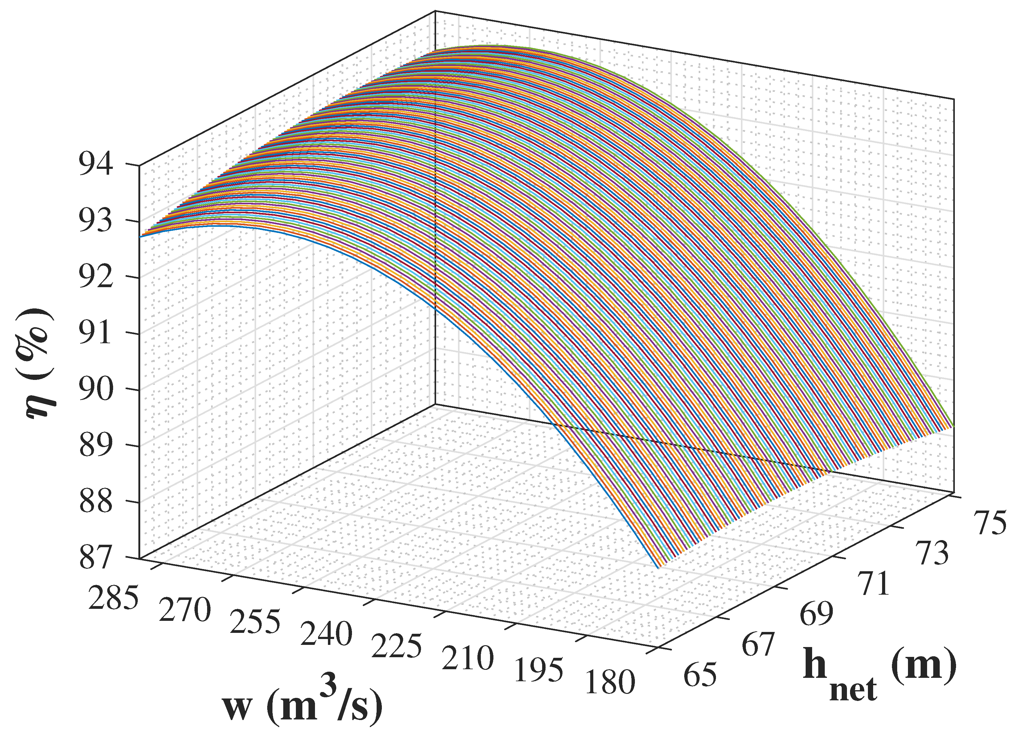
It is important to highlight that undesired spillage indications are consequences of the hill-shaped form intrinsic to hydraulic turbine efficiency curves, regardless of the turbine type. Figure 1 depicts the efficiency function for $G_2$’s turbines. In this curve, one can notice that if the water flow (w) is equal to 195 m${}^3$/s, the efficiency reaches higher values as the net head ($h_{net}$) decreases from 75 to 73 m. For any $h_{net}$ value, the efficiency reaches higher values as w increases from 195 to 225 m${}^3$/s. Intuitively, spilling water from the reservoir causes a decrease in its level and an increase in the downstream basin level, hence decreasing the net head and requiring more water to flow through the turbines to meet the given power demand. In other words, no matter the turbine type and as long as the function is given by a hill-shaped curve, spillage can lead to higher efficiency depending on the operating point.

The affirmations presented in the previous paragraph, in conjunction with the development exposed in this section, make it clear that the HPP operation optimizer can indicate spillage even when the reservoir is not at its maximum capacity, leading to a waste of resources as a consequence. As the cause of these indications relates to the hill-shaped efficiency curve, they can occur in any HPP in which this type of function rules the turbines. This affirmative is true regardless of any other operation characteristic, such as the number of generating units (either being identical or not) in the power plant, the length of the planning horizon, and the study context concerning single or multiple HPPs. In summary, this study contributes to the development of coherent operation optimization codes, which can enable more reliable results, help save resources, and prevent operators from making questionable decisions regarding reservoir water spillage.

Regarding the approach presented in [3] (Equations (18)–(20)), since it only allows water to be spilled when the reservoir volume (v) is greater than or equal to $v^{max}-ϵ$, the method tends to indicate less undesired spillage in comparison with the results presented in Table 5, Table 7 and Table 8. However, the optimization can still result in excessive water usage if non-null spillage values are feasible, as exposed in this paper. In other words, this approach does not prevent the optimizer from indicating wasteful spillage. Furthermore, it is possible that spilling water only when $v\ge v^{max}-ϵ$ is not enough to keep the reservoir below or at its maximum capacity if $ϵ$’s value is too low, hence making it impossible for the optimizer to reach convergence. Therefore, it is more appropriate to adapt the formulation and apply a water outflow-based objective function.

The limitation of this work relates exclusively to the simple modeling of turbine efficiency curves (Equation (5)), which was performed by second-order polynomial fitting, as in [11]. In general, these curves are provided by turbines manufacturers as a data set that contains numerous three-dimensional samples (net head, water flow, and efficiency), which are then used to obtain a “black box” that grants the efficiency (given net head and water flow values). For instance, these samples can be fitted by one polynomial (higher polynomial order implies higher accuracy), or by multiple polynomials obtained via segmentation of the original data set. More complex and precise approaches to model turbine efficiency may impact the exposed undesired spillage indications regarding their magnitude, which defines a possibility of future investigations concerning this subject. However, no matter the model, these indications are always prone to happen when applying power losses-based objective functions due to the hill-shaped efficiency curve, as explained in this paper.

For the readers who intend to apply a monetary cost-based objective function that includes start-up and shutdown costs, though considering spillage as a decision variable, writing part of the objective function as costs related to power losses can be troublesome, as shown in this paper. To engage in such an approach and avoid undesired spillage indications, one could set monetary values to the storage water, thus making it possible to use water outflow values instead of power losses in the objective function, as in [2].

The “BenchmarkTools” Julia package was used to carry out a computational effort analysis of the simulations, which were performed in a computer with the following characteristics: AMD Ryzen 5 2600 six-core processor with 3.4 GHz, 8 GB of RAM, and a 64 bits Windows 10 operational system.

Table 14. Duration of simulations (mean ± standard deviation).

Objective Function	Scenario 1	Scenario 2	Scenario 3
WO	221.46 ± 10.37 s	322.55 ± 17.41 s	1.28 ± 0.06 s
PL	233.99 ± 9.74 s	299.04 ± 11.38 s	1.31 ± 0.06 s

exposes the mean and standard deviation values obtained by performing four simulations of each scenario. Both power losses (PL) and water outflow (WO) objective functions were considered.

In Table 14, the low standard deviation values (in comparison to mean values) show the consistency of the optimization lengths given a particular scenario and objective function. In contrast to scenarios 1 and 2, scenario 3 presents power demands that vary lightly throughout the day (see Table 1, Table 2 and Table 3). Such characteristic simplifies the process and is responsible for scenario 3’s much lower optimization duration. Although both scenarios 1 and 2 present significant demand variation, the latter is the only one in which water must be spilled from the reservoir so that its volume remains within its bounds. The assignment of non-null values to spillage decision variables also impacts computational effort, which justifies scenario 2’s higher optimization duration. Regarding the objective functions, WO required less time in scenarios 1 and 3, whereas PL prevailed in scenario 2. However, the differences were considerably small in all cases. In general, the required times to optimize the daily operation of the power plant were all viable, with the longest one being equivalent to less than six minutes.

4. Conclusions

This paper explained the cause of undesired spillage indications when optimizing the operation of hydroelectric power plants. Analysis of mathematical aspects showed that such a phenomenon is related to the nature of hydraulic turbine efficiency curves. In specific cases, power losses-based objective functions lead the optimizer to reach higher efficiency levels when spilling reservoir water and, consequently, reducing the gross head and increasing turbines water flow. Results have shown that reservoir resources can be wasted according to the objective function applied in the problem formulation when spillage is considered a decision variable. It is emphasized that renewable energy sources greatly contribute to environmental balance. Therefore, properly optimizing their operation helps secure resources for future demands. By exposing the studied matter, the authors of this paper intend to raise awareness on its cause so that fellow researchers more quickly identify similar situations. For future studies, it is intended to assess how much different turbine efficiency models impact the magnitude of undesired spillage indications.