Article

Automatic P2P Energy Trading Model Based on Reinforcement Learning Using Long Short-Term Delayed Reward

Department of Electronic Engineering, Inha University, Incheon 22212, Korea
*
Author to whom correspondence should be addressed.
Energies 2020, 13(20), 5359; https://doi.org/10.3390/en13205359
Submission received: 3 September 2020 / Revised: 2 October 2020 / Accepted: 5 October 2020 / Published: 14 October 2020
(This article belongs to the Special Issue AI Applications to Power Systems)

Abstract

:
Automatic peer-to-peer energy trading can be defined as a Markov decision process and designed using deep reinforcement learning. We consider prosumer as an entity that consumes and produces electric energy with an energy storage system, and define the prosumer’s objective as maximizing the profit through participation in peer-to-peer energy trading, similar to that of the agents in stock trading. In this paper, we propose an automatic peer-to-peer energy trading model by adopting a deep Q-network-based automatic trading algorithm originally designed for stock trading. Unlike in stock trading, the assets held by a prosumer may change owing to factors such as the consumption and generation of energy by the prosumer in addition to the changes from trading activities. Therefore, we propose a new trading evaluation criterion that considers these factors by defining profit as the sum of the gains from four components: electricity bill, trading, electric energy stored in the energy storage system, and virtual loss. For the proposed automatic peer-to-peer energy trading algorithm, we adopt a long-term delayed reward method that evaluates the delayed reward that occurs once per month by generating the termination point of an episode at each month and propose a long short-term delayed reward method that compensates for the issue with the long-term delayed reward method having only a single evaluation per month. This long short-term delayed reward method enables effective learning of the monthly long-term trading patterns and the short-term trading patterns at the same time, leading to a better trading strategy. The experimental results showed that the long short-term delayed reward method-based energy trading model achieves higher profits every month both in the progressive and fixed rate systems throughout the year and that prosumer participating in the trading not only earns profits every month but also reduces loss from over-generation of electric energy in the case of South Korea. Further experiments with various progressive rate systems of Japan, Taiwan, and the United States as well as in different prosumer environments indicate the general applicability of the proposed method.

1. Introduction

In energy markets, the number of prosumers, i.e., the entities that generate and consume electric energy, has been increasing owing to the proliferation of distributed energy resources (DERs), such as photovoltaic (PV) systems, owned by traditional energy consumers. Accordingly, the proportion of microgrids in the power system has been expanding. In response, the incorporation of information and communication technology into existing power grids is becoming more important, and the core technologies of smart grid systems such as energy storage systems (ESSs), power conversion systems, mobility, and energy monitoring systems have advanced dramatically. In addition, studies on peer-to-peer (P2P) energy sharing or trading based on these core technologies between prosumers have been increasing [1,2,3,4,5,6,7,8,9,10,11], among which studies on P2P trading based on reinforcement learning (RL) [12] are actively being conducted [13,14,15,16]. Chen and Su [13] highlighted to the role of energy brokers in the localized event-driven market (LEM) because small-scale electricity consumers and prosumers typically take a long time to search for trading partners, and, therefore, pure P2P mode is not suitable. Nevertheless, these brokers aim to maximize profits in the LEM and determine the optimal action by using the Q-learning algorithm of RL [13]. In addition, it was suggested that the LEM participation strategy for energy trading can be modeled as a Markov decision process (MDP) and solved through a deep Q-network (DQN) [14]. Similarly, Chen and Bu [15] proposed a solution to the decision-making problem of microgrids in the LEM through a DQN-based P2P energy trading model of deep RL (DRL), and Liu et al. [16] applied a DQN for autonomous agents in the consumer-centric electricity market.
As such, recent studies on P2P energy trading define the strategy for participating in the trading as an MDP and apply RL or DRL to find the optimal trading participation strategy. This is because it is important to choose a reasonable and effective trading strategy in P2P energy trading. Therefore, the performance of RL, which is responsible for presenting the trading strategy, is very important for automatic P2P trading. However, most previous works [13,14,15,16] only applied RL or DRL to solve the MDP on energy trading, but did not consider the network modification of RL as they only considered the characteristics of energy trading to effectively solve it.
We aim to maximize the profits of the prosumer through automatic P2P energy trading, which is the same as that of stock trading algorithms. Therefore, we use the RL-based automatic trading algorithm used in stock trading to implement the automatic energy trading model. Our model provides optimal trading action based on independent prosumer ESS information, electricity generation, and consumption information for each designated trading time unit. Assuming that there exists a mechanism for the physical transaction of the P2P energy trading results, we present an implementation of an RL-based trading model for the automation of P2P energy trading and an effective network configuration by considering the unique factors of P2P energy trading.
In this paper, we propose a long short-term delayed reward (LSTDR) method that improves the existing delayed reward method of the RL network. LSTDR is a method that utilizes both short-term and long-term delayed rewards, enabling effective analysis of the long-and short-term patterns of trading environment information. To effectively analyze time-dependent information, we use a DQN based on a long short-term memory (LSTM) as the training model. The proposed method focuses on maximizing individual prosumer’s profit based on noncooperative game theory [17] without considering the optimization of the overall benefits of all prosumers, so it is not directly related to Pareto optimality [18,19]. It does not consider the gain of consumers who do not generate electric energy either. Nevertheless, individual prosumers can benefit from adopting the proposed trading strategy at the same time reduce the overall energy generation of the grid which may potentially benefit consumers as well.
The remainder of this paper is organized as follows. Section 2 discusses the background information of the global energy market and P2P energy trading based on DRL and the existing works. Section 3 explains the difference between stock trading and energy trading, discusses the schemes for the modification of the automatic trading network by considering them, and proposes a new evaluation criterion for the trading strategy of LSTDR for RL. Section 4 presents the trading environment and experimental data for the performance evaluation of our proposed model. Section 5 discusses the experimental results. Finally, Section 6 concludes this paper.

2. Background and Related Works

2.1. Global Energy Market

Most countries fall into the category of energy producers which can produce energy from energy sources such as coal, oil and gas, or from renewable energy sources (RES). Energy produced in each country covers each domestic energy demand, and additionally needed or remaining energy after production is imported or exported to other countries, which activates the global energy markets [20]. In the scenario of the International Energy Agency (IEA)’s “World Energy Outlook 2019 (https://www.iea.org/reports/world-energy-outlook-2019)”, the demand for primary energy in the global energy market will continue to increase every year, led by emerging economies such as China and India, while demand for primary energy will decrease in the developed countries, while the share of renewable energy will increase gradually for a low carbon emission to cope with the climate change. In addition, among the energy markets, the demand for electricity in the global electricity market will show the similar pattern, and the proportion of renewable energy in the supply is expected to increase significantly. The expansion of supply and demand for renewable energy in the electricity market may lead to the advancement of renewable energy generation technologies and the spread of supply [21], and increase the number of prosumers participating in the energy market for small-scale electricity generation through RES.
Each country provides benefits through various policies to promote electricity consumers to become prosumers. Most developed countries provide an environment where prosumers can generate profits by reducing electricity bills by increasing their self-consumption rate through self-generated electricity, or by selling it [22]. However, since the methods of electricity rate systems applied to each country are not all the same, even if prosumers in different countries have the same amount of consumption and generation, their profits can differ. For example, in two different countries with progressive rate system, if one country has a narrow range of progressive stages and a higher progressive rate compared to the other, the prosumers included in this country may gain less profits than those in the other country, even if they have less consumption and more electricity generation. This is an example of South Korea and the United States. In South Korea, the rate at the first progressive stage is lower than in the United States, but the progressive range is very narrow compared to the United States and the rate of increase in progression is much higher, resulting in higher electricity bills in South Korea compared to the same amount of electricity used in summer. Thus, the strategies of prosumers participating in trading in the electricity market should vary from country to country.

2.2. Peer-to-Peer Energy Trading

In P2P energy trading, the main agent is the prosumer, who produces and consumes energy and exchanges with other prosumers for surplus electricity that is overproduced after consumption [23]. Such P2P energy trading takes place in small DERs such as dwellings, factories, schools, and offices [6,7]. Unlike in the indirect trading method of conventional energy trading, where trading is performed through brokers offering wholesale or bundled services, in P2P energy trading, prosumers can trade directly with other prosumers (or consumers). Underscoring the strength of P2P energy trading, Tushar et al. [4] suggested that the development of this type of trading can lead to potential benefits for prosumers, such as earning profits, reducing electricity bills, and lowering their dependency on the grid. They also mentioned the importance of modeling the prosumer’s decision-making process, noting that the system for energy trading requires reasonable modeling of each participant’s decision-making process that can generate greater benefits for the entire energy network while considering human factors such as rationality, motivation, and environmental affinity for the trading. Therefore, it is important for P2P energy trading to set the direction and to model a strategy, and game theory [24] can be applied to this. Game theory can be divided into two main concepts: noncooperative game theory [17] and cooperative game theory [25]. In P2P energy trading, a noncooperative game sets a strategy with the goal of maximizing its own profits without the need to share and collaborate with other prosumers participating in the trading during the decision-making process. In contrast, in a cooperative game, for the benefit of all independent prosumers, they become the subject, share strategies and coordinate their own strategy choices. Therefore, even in the same energy trading environment, the game theory applied according to the purpose of the prosumer is different. In this study, we model the trading strategy on the basis of the noncooperative game theory that maximizes profits from the individual prosumer’s point of view. Figure 1 compares the structures of non-P2P energy trading and the P2P energy trading.

2.3. Markov Decision Process

The MDP is a discrete time probability control process that mathematically models and analyzes decision making, and it is designed according to the first-order Markov assumption that the current state is affected only by the previous state [26]. P2P energy trading is a decision-making problem in which a decision to participate in a trading can be defined as an MDP in an environment containing high-dimensional information. The MDP can be defined by the following five elements:
  • State Space S: This is the set of states s of the agent, which is the decision maker of a given environment E. In P2P energy trading, it is the state of the prosumer, which is the agent in a given trading environment, and includes the environmental information of the prosumer, such as energy generation, consumption, and energy reserves.
  • Action Space A: This is the set of all actions that the agent can select in a given state s. In P2P energy trading, the set of actions that a prosumer can select in a given state includes the actions for participating in the trading, such as buy, sell, and hold.
  • Reward R: This is the reward that the agent obtains from each action in a given state. Reward is typically a scalar, and depending on how the condition is set in each state, the reward obtained by the agent varies. There are two types of rewards: immediate reward, which is rewarded for the outcome of the next state, and delayed reward, which is rewarded for future results that are affected by the current behavior [27].
  • State Transition Probability Matrix P: State transition probability is the probability of transitioning from one state to another (or to the same state) and P is the matrix that defines the state transition probabilities in all states.
  • Discount Factor γ : This is an element that plays a role in making the reward value of the future viewed from the present smaller according to the time distance from the present, considering that the future behavior is less affected by the present state as it returns with time. It has a value between 0 and 1.
Finally, a policy π to solve the MDP can be expressed through the above five elements and can be obtained through dynamic programming [28] or RL. Figure 2 shows the basic process of the MDP.

2.4. Deep Reinforcement Learning

DRL is a method that utilizes deep learning (DL) in RL algorithms [29]. RL algorithms optimize a policy using various approaches to find the optimal policy for the given goal. Representative algorithms of RL include SARSA [30], policy gradient [31], and Q-learning [32], and these algorithms update the main learning parameters using a function approximator to find the optimal policy [33]. DRL optimizes the policy by replacing this function approximator with DL. Accordingly, it is possible to effectively learn from a huge amount of data, and this has the advantage of improving the learning performance by applying various DL methods.

2.4.1. Deep Q-Networks

DQN [34] is a DRL algorithm that combines a deep neural network (DNN) with a Q-learning algorithm of RL. For Q-learning, a policy is recorded in the Q-table so that it can output the optimal action in each state of the agent [32]. However, this tabular recording of policy requires more memory as the amount of data increases or the dimension of the data increases. To solve this problem, function approximator is used to define the Q-function through parameters other than the table. The DQN uses the DNN as the function approximator [34] and applies the experience replay method to improve the data learning efficiency. To reduce the inefficiency of learning due to the correlation of adjacent learning data, the experience replay method stores the information about the agent’s actions and the resulting state changes and rewards as a tuple-type transition in a buffer called replay memory and uses it for sampling during training. Therefore, it is possible to prevent a situation that falls into a local minimum by randomly selecting and using the transitions obtained in various environments during training. Algorithm 1 shows the overall algorithm structure of DQN proposed in [34].
Algorithm 1 Deep Q-learning with Experience Replay
  • Initialize replay memory D to capacity N
  • Initialize action-value function Q with random weights
  • for episode = 1, M do
  •     Initialise sequence s 1 = { x 1 } and preprocessed sequence ϕ 1 = ϕ ( s 1 )
  •     for t = 1, T do
  •         With probability ϵ select a random action a t
  •         otherwise select a t = max a Q ( ϕ ( s t ) , a ; θ )
  •         Execute action a t in the emulator and observe reward r t and input x t + 1
  •         Set s t + 1 = s t , a t , x t + 1 and preprocess ϕ t + 1 = ϕ ( s t + 1 )
  •         Store transition ( ϕ t , a t , r t , ϕ t + 1 ) in D
  •         Sample a random minibatch of transitions ( ϕ j , a j , r j , ϕ j + 1 ) from D
  •         Set y j = r j for terminal ϕ j + 1 r j + γ max a 0 Q ( ϕ j + 1 , a 0 ; θ ) + R total for non - terminal ϕ j + 1
  •         Perform a gradient descent step on ( y j Q ( ϕ j , a j ; θ ) ) 2
  •     end for
  • end for

2.4.2. Long Short-Term Memory

LSTM is a recurrent neural network (RNN) model in DL; it is effective for analyzing time-series data and is used for solving the gradient vanishing problem that occurs in vanilla RNN [35]. LSTM has a structure in which one memory cell c t and three gates (i.e., input gate i t , forget gate f t , and output gate o t , all at time t) that control the information flow are added to the vanilla RNN structure, so that long-term information can be effectively handled. Each gate operates in a different role [36]. The input gate determines how much the current information is reflected and stored in the memory cell, and the forget gate determines how much past information is forgotten and transferred to the memory cell. The output gate determines how much information is reflected and outputs the information currently stored in the memory cell. The operation of these gates is determined by an activation function σ (typically sigmoid or hyperbolic tangent) in each state. In this way, it is possible to effectively deal with time-series information because the information is updated by determining the importance and association of the information over time at each gate. The overall operating structure of LSTM can be expressed by the following equations [35]:
i t = σ g ( w i x t + U i h t 1 + b i ) ,
f t = σ g ( w f x t + U f h t 1 + b f ) ,
o t = σ g ( w o x t + U o h t 1 + b o ) ,
c t = f t c t 1 + i t σ c ( w c x t + U c h t 1 + b c ) ,
h t = o t σ h ( c t ) .
For the input sequence x = { x 1 , x 2 , x 3 , . . . , x T } in Equation (Section 2.4.2), x t represents the input at time t; U i , U f , U o , U c , w i , w f , w o and w c are the weight matrices; and b i , b f , b o , and b c are the bias vectors, all of which are the parameters that are updated during training. Finally, c t and hidden layer output h t , which is the information transmitted to the next state, are calculated through the Hadamard product (∘), which is the element-wise product of the output of each gate and information c t 1 and h t 1 transmitted from the previous state. Figure 3 shows the architecture of LSTM.

3. Proposed Approach

Stock trading is the buying and selling of stocks. It is a nonphysical type of trading as there is no exchange of physical products. In stock trading, the agents participating in the trading aim to maximize their gains through trading at the optimum time using the market price of stocks that fluctuate in real time. Accordingly, whether or not the agents will participate in the trading mostly depends on the market price of the stock. Figure 4 shows the algorithm of automatic stock trading based on DRL.
Unlike stock trading, energy trading has additional factors that affect the trading conditions. First, the electricity subject to energy trading can be generated and consumed by the prosumers; therefore, its reserves can change in real time even when they are not traded, unlike stocks whose reserves change only by trading. Therefore, it is necessary to redefine the evaluation criterion of energy trading to make it different from that of stock trading, which uses the portfolio of the sum of only the currency values of the assets held. Second, unlike stocks, which are virtually traded, electricity is physically traded, and, therefore, there is a trading time until a trading is made and terminated. Third, when electricity is charged or discharged, losses occur depending on the ESS efficiency, and, therefore, the actual trading result will be different from the initial trading volume. Considering these, we propose strategies for designing a model suitable for automatic P2P energy trading. The automatic energy trading model adopts the existing automatic stock trading algorithm and modifies it to match the specifics of energy trading.

3.1. Definition of the P2P Energy Trading Evaluation Criterion

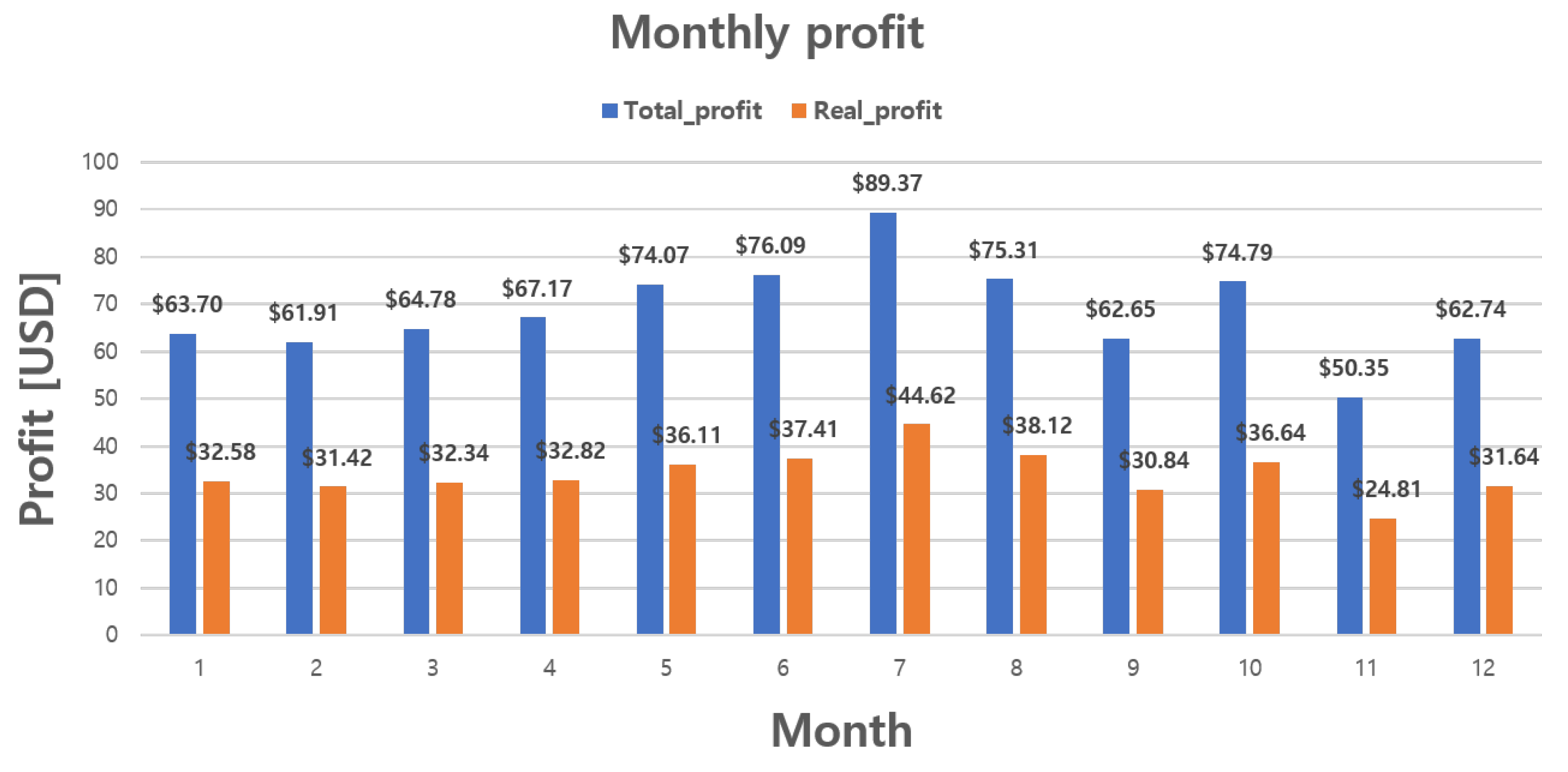
The electricity reserves in the ESS resulting from the energy generation and consumption of prosumer constantly change even if there is no trading, and the energy trading determines the trading action according to the reserves in the ESS changed by the previous trading, consumption, or generation. Therefore, if the currency value of the assets held in stock trading is used as an evaluation criterion of the trading, it is impossible to accurately evaluate the trading results owing to the changes in energy generation and consumption. Therefore, we define an evaluation criterion as the sum of the gains from participating in P2P energy trading compared with not participating in it.
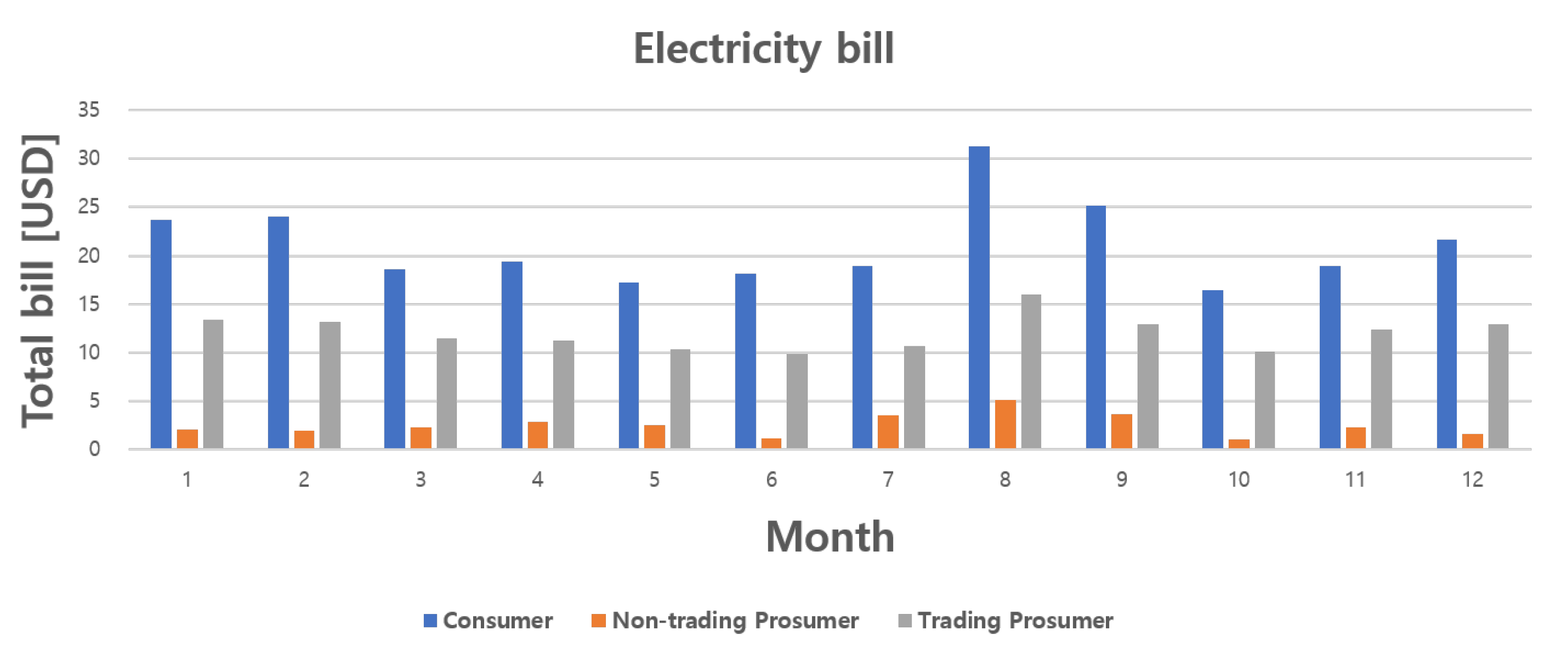
The total profit from participating in the P2P energy trading proposed in this paper is defined as the sum of four gains. The first gain is the change in the electricity bill. When energy trading is completed, since the result of the trading changes the amount of electricity held in the ESS, the amount of electricity available to the prosumer in the ESS is changed, and the amount of electricity supply used is also changed accordingly. For example, if the amount of electricity held in the ESS is less than the amount consumed, the electricity bill can be reduced by purchasing electricity through P2P energy trading rather than through the supply electricity. Conversely, while the amount of electricity held in the ESS is greater than the amount consumed, selling through P2P energy trading can result in profit, although it may involve the use of supply electricity, which may increase the electricity bill. Therefore, if only the gain from the trading is considered without the electricity bill, there may be a situation in which additional electricity bills are paid more than the gain from the trading, resulting in loss. The gain from the change in electricity bill can be expressed as follows:
G b i l l ( S p ( t ) ) = B o ( S o ( t ) ) B p ( S p ( t ) ) ,
where t = 1 , 2 , 3 , , T ; B o ( S o ( t ) ) is the electricity bill paid by the prosumer who does not participate in P2P energy trading in state S o ( t ) and B p ( S p ( t ) ) is the electricity bill paid by the prosumer who participates in P2P energy trading in state S p ( t ) . In both situations, the difference in electricity bills is G b i l l ( S p ( t ) ) , which is the gain from the change in the electricity bill for participating in energy trading, where t is the number of states that have elapsed from the start of the electricity bill calculation to the hour-by-hour period, and T is the total number of states from the time the final electricity bill is calculated. We assume that the time before the trading is established, the electricity is transferred, and the ESS is completely charged/dischargid is within 1 h, thereby setting the trading participation decision interval to 1 h. Therefore, 
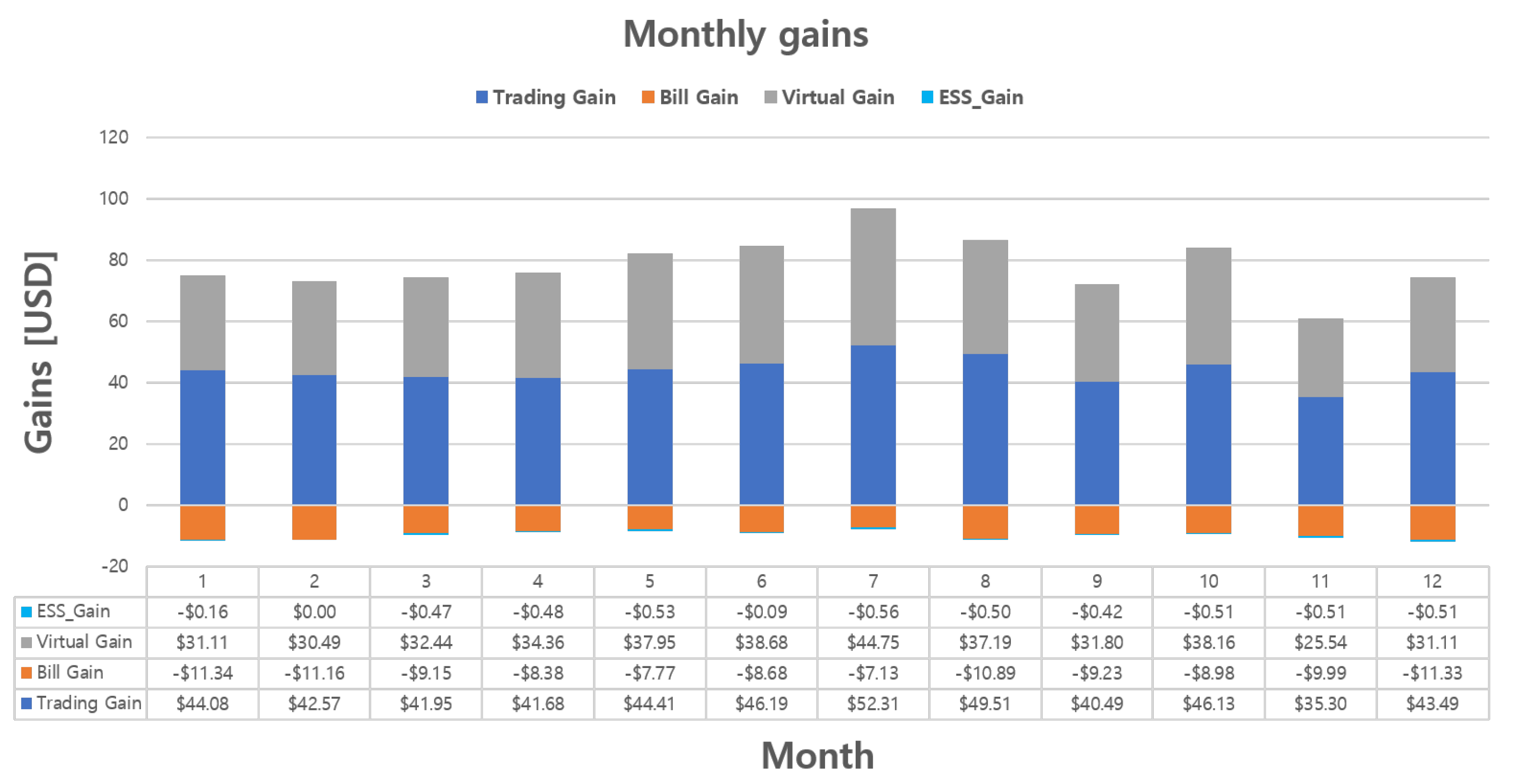
t increases in units of 1 h. The second gain is the trading gain from P2P energy trading. When a prosumer participates in a P2P electricity trading, the prosumer takes one of three actions: buying, selling, and nonparticipation, and the prosumer’s assets change as a result of the trading. The amount of change in these assets is equal to the gain achieved only through trading, and it can be defined as
0 Q b ( S p ( t ) ) 1 / η · E m a x ,
0 Q s ( S p ( t ) ) η · E m a x ,
M b ( S p ( t ) ) = ( 1 + ξ ) · ( P ( S p ( t ) ) · Q b ( S p ( t ) ) ) ,
M s ( S p ( t ) ) = ( 1 ξ ) · ( P ( S p ( t ) ) · Q s ( S p ( t ) ) ) ,
M t r a d e ( S p ( t ) ) = k = 1 t M s ( S p ( k ) ) k = 1 t M b ( S p ( k ) ) ,
G t r a d e ( S p ( t ) ) = M t r a d e ( S p ( t ) ) M t r a d e ( S o ( t ) ) ,
G t r a d e ( S p ( t ) ) = M t r a d e ( S p ( t ) ) ,
where E m a x represents the maximum storage capacity of the ESS, and η represents the efficiency of the ESS. Q b ( S p ( t ) ) and Q s ( S p ( t ) ) represent the trading purchase and sale volume, respectively, and  P ( S p ( t ) ) represents the trading price. M b ( S p ( t ) ) and M s ( S p ( t ) ) represent the cost spent on purchases and the profits from sales, respectively. At this time, ξ represents the trading fee. M t r a d e ( S o ( t ) ) and M t r a d e ( S p ( t ) ) , which are the total amount of asset changes through trading, are calculated as the difference between the total amount of revenue and the expenditure up to t. When the prosumer does not participate in P2P trading, the asset changes through trading M t r a d e ( S o ( t ) ) are zero, and, therefore, the gain from the P2P energy trading G t r a d e ( S p ( t ) ) is equal to M t r a d e ( S p ( t ) ) . Since the trading is based on the ESS, the amount of electricity that can be traded is limited. Therefore, the trading volume should consider the amount of electricity held in the ESS or the remaining storage capacity of the ESS, and it cannot exceed the maximum ESS capacity. In addition, trading fees may also be considered in P2P energy trading, which should be further considered in the settlement of trading costs. The third gain is for virtual losses from over-generation. If electricity is generated while the electricity in the ESS is fully charged, the generated electricity cannot be stored in the ESS, resulting in losses. However, this can be prevented through the sales from P2P energy trading before these losses occur. Therefore, it is possible to perform an efficient trading action considering the electricity generation by the prosumer and the losses from over-generation depending on whether or not P2P energy trading is involved. The gain on virtual losses from over-generation can be expressed as follows:
V g a i n ( S p ( t ) ) = η · ( L o ( S o ( t ) ) L p ( S p ( t ) ) ) · P ( S p ( t ) ) ,
G v i r t u a l ( S p ( t ) ) = k = 1 t V g a i n ( S p ( k ) ) ,
where L o ( S o ( t ) ) and L p ( S p ( t ) ) are the amount of electricity loss from over-generation, and V g a i n ( S p ( t ) ) is the instantaneous gain on the currency value of the virtual loss in state S p ( t ) . G v i r t u a l ( S p ( t ) ) is the cumulative gain from reducing over-generation. Setting up a trading strategy in such a way as to reduce losses from over-generation not only can reduce the losses of prosumers but also can have the effect of reducing the total amount of supply electricity on the power system. The fourth gain is the change in the currency value of the amount of electricity held in the ESS. The electricity held in the ESS is the result of consumption, generation, and trading, and it includes the result of the changes due to the trading actions. The gain from the change in the currency value of the amount of electricity in the ESS can be expressed as follows:
C g ( S o , p ( t ) ) = η · G e n e r a t i o n ,
D c ( S o , p ( t ) ) = 1 / η · C o n s u m p t i o n ,
C b ( S p ( t ) ) = η · Q b ( S p ( t ) ) ,
D s ( S p ( t ) ) = 1 / η · Q s ( S p ( t ) ) ,
E ( S o ( t ) ) = E ( S o ( t 1 ) ) + C g ( S o ( t ) ) + D c ( S o ( t ) ) ,
E ( S p ( t ) ) = E ( S p ( t 1 ) ) + C g ( S p ( t ) ) + D c ( S p ( t ) ) + C b ( S p ( t 1 ) ) + D s ( S p ( t 1 ) ) ,
G e s s ( S p ( t ) ) = η · ( E ( S p ( t ) ) E ( S o ( t ) ) ) · P ( S p ( t ) ) ,
where C g ( S o , p ( t ) ) and D c ( S o , p ( t ) ) respectively represent the amount of ESS charged and discharged owing to the generation and consumption of the prosumer from state S o , p ( t ) to state S o , p ( t 1 ) . Moreover, C b ( S p ( t ) ) and D s ( S p ( t ) ) respectively represent the amount of electricity charged and discharged by the prosumer through P2P energy trading. E ( S o ( t ) ) and E ( S p ( t ) ) represent the amount of electricity in the ESS. In addition, because the effect (charge or discharge) of the trading result in state S p ( t 1 ) is not immediately apparent but is shown in the next state S p ( t ) , the amount of electricity in the ESS E ( S p ( t ) ) after the prosumer’s P2P energy trading utilizes the trading volume in the previous state S p ( t 1 ) rather than the current trading volume in state S p ( t ) . G e s s ( S p ( t ) ) represents the gain from the currency value of the electricity held in the ESS. Finally, the profit G ( S p ( t ) ) for participating in P2P energy trading, which has been redefined as the trading evaluation criterion, is defined as follows:
G ( S p ( t ) ) = G b i l l ( S p ( t ) ) + G t r a d e ( S p ( t ) ) + G e s s ( S p ( t ) ) + G v i r t u a l ( S p ( t ) ) .

3.2. Long Short-Term Delayed Reward

MDPs that have a continuous environment such as automatic trading do not have exact termination points, unlike MDPs that have an episode’s termination point, such as mazes, Atari games, and CartPoles [37]. Therefore, in the case of the existing RL-based stock trading [38], the RL structure is designed to generate the termination points of learning by providing a delayed reward [27] when a certain amount of portfolio gain or loss is achieved during the trading. However, we considered various external factors affecting energy trading when defining the evaluation criterion for energy trading in Section 3.1 and utilized the gain from electricity bills. The electricity bill is set according to the amount of electricity used each month. Accordingly, we aimed to determine the monthly gains, and, for this purpose, we set the time that the delayed reward is the output of automatic energy trading at the end of the period when the electricity price is set so that the termination point of the episode is generated every month. Similarly, most of the papers on energy trading set the trading strategy by designating a certain size (period) for an episode [13,14,39,40], and the policy is updated by using the immediate rewards that occur in every state in episode and the delayed reward generated at the termination point of the episode. The delayed reward value only determines the end point of the episode to proceed with the policy update, but is not directly used for policy update. The policy update reflects the impact on the future by applying a discount factor to each of the immediate rewards from the current state to the state in which the delayed reward occurred.
Such a one-month delayed reward assignment, however, can make learning difficult for short-term patterns that occur within a month. To compensate for this, we design an additional delayed reward to include the case when an increase or decrease in the profit that we defined occurs above a certain threshold as in the stock trading method. At this time, the delayed reward is not provided whenever an increase or decrease occurs above a certain threshold, such as in stock trading, but is added to the final delayed reward by utilizing the number of occurrences of the increase or decrease within a month. Finally, the delayed reward information is utilized when deciding on the action in each state to ensure that the outcome of a month’s trading affects the learning direction in the training. For this, the obtained delayed reward is added to the Q-function updated through the neural network. By applying the delayed reward method of stock trading to energy trading, we enable the DNN in RL at the beginning of the learning to focus on very short-term patterns (because of the generation of batch data based on the delayed reward that occurs every short period of time) and then to find that the monthly pattern is important while finding the overall training direction only after a great deal of training has progressed. However, to do it, we can set the monthly term as a unit of training (which results in a delayed reward every month) so that we can train from the beginning of the training in a way that fits our goals. In addition, the ratio of the profit and the number of trades was utilized to add to the final delayed reward. By doing so, when delayed reward occurs owing to a profit above a threshold, we can direct the trading model to effectively maximize the profit while giving a higher score continuously to a situation where more gain is obtained instead of the same delayed reward score. Therefore, we propose an LSTDR method for delayed reward by considering long-term patterns of 1 month and short-term patterns in the long-term. Figure 5 shows the structure of the proposed automatic P2P energy trading scheme. Algorithm 2 shows the overall algorithm structure for the energy trading with LSTDR method.
Algorithm 2 Energy trading with the LSTDR method
  • Initialize replay memory D to capacity N
  • Initialize action-value function Q with random weights
  • for epoch = 1, M do
  •     Initialise sequence s 1 = { x 1 } and preprocessed sequence ϕ 1 = ϕ ( s 1 )
  •     Initialize G t o t a l (total gain) to zero and G b a s e (base gain) to non-zero
  •     Initialize C s (count value for the occurrence of non-zero R s (short-term delayed reward)) to zero
  •     Initialize S s (cumulative value of R s ) to zero
  •     Initialize P m (cumulative value of the unit trading price) to zero
  •     Initialize N t r a d e (number of times prosumer participated in the trading) to zero
  •     Initialize N s (count value for the number of states in a month) to zero
  •     Set g s (threshold value of the short-term profit) to user’s desired value (we set it to 0.2)
  •     Set g m (threshold value of the monthly profit) to user’s desired value (we set it to 0.25)
  •     for t = time of the first training data, time of the last training data do
  •          N s + = 1
  •         With probability ϵ select a random action a t
  •         otherwise select a t = max a Q * ( ϕ ( s t ) , a ; θ )
  •         Execute action a t in the emulator and observe immediate reward r t and environment x t + 1
  •         Set s t + 1 = s t , a t , x t + 1 and preprocess ϕ t + 1 = ϕ ( s t + 1 )
  •         Store transition ( ϕ t , a t , r t , ϕ t + 1 ) in D
  •         Update G t o t a l with G b i l l , G t r a d e , G e s s and G v i r t u a l
  •         Update B o (prosumer’s current electricity bill when not participating in the P2P trading)
  •         Update P m and N t r a d e
  •         if G b a s e is equal to or greater than zero then
  •              if G t o t a l is equal to or greater than ( 1 + g s ) · G b a s e then R s is 1
  •              else if G t o t a l is greater than ( 1 g s ) · G b a s e and less than ( 1 + g s ) · G b a s e then R s is 0
  •              else R s is -1
  •              end if
  •         else
  •              if G t o t a l is equal to or greater than ( 1 g s ) · G b a s e then R s is 1
  •              else if G t o t a l is greater than ( 1 + g s ) · G b a s e and less than ( 1 g s ) · G b a s e then R s is 0
  •              else R s is -1
  •              end if
  •         end if
  •          S s + = R s
  •         if R s is not zero then C s + = 1 and G b a s e = G t o t a l
  •         end if
  •         if t is the end of the month then
  •               R a = ( ( G t o t a l G v i r t u a l ) / N t r a d e ) · ( N s / P m )
  •              if ( G t o t a l G v i r t u a l ) is equal to or greater than B o · g m then
  •                     R l (long-term delayed reward) is R a + 1
  •              else if ( G t o t a l G v i r t u a l ) is greater than zero and less than B o · g m then R l is R a
  •              else R l is R a 1
  •              end if
  •               R t o t a l is α · R l + ( 1 α ) · ( S s / C s )       ( α is a weight factor between 0 and 1)
  •              Initialize G t o t a l , G b a s e , C s , S s , P m , N s , N t r a d e
  •         else R t o t a l is zero
  •         end if
  •         if R t o t a l is non-zero then
  •              Sample a random minibatch of transitions ( ϕ j , a j , r j , ϕ j + 1 ) from D
  •                Set y j = r j + R t o t a l for terminal ϕ j + 1 r j + γ max a 0 Q ( ϕ j + 1 , a 0 ; θ ) + R t o t a l for non - terminal ϕ j + 1
  •            Perform a gradient descent step on ( y j Q ( ϕ j , a j ; θ ) ) 2
  •         end if
  •     end for
  • end for

4. Experiments

In our work, we defined the trading environment for the evaluation of the proposed P2P automatic energy trading model and generated the experimental data accordingly. The experiment was conducted under the assumption that P2P energy trading exists in South Korea, and the public data in South Korea were utilized for the data generation. In the experiment, we verified the validity of the proposed LSTDR method and confirmed the profit that the prosumer would gain by participating in the trading through the proposed P2P automatic energy trading model. In the first experiment, we compared the results of three delayed reward methods: the short-term delayed reward (STDR) method [27], which is a delayed reward method used in stock trading; long-term delayed reward (LTDR) method [13,14,39,40], which generates a termination point every month to provide delayed reward at that time; and the LSTDR method, which utilizes both of these methods and is the one proposed in this paper. The second experiment compared the prosumers who did and did not participate in the trading to confirm the benefits of participating in P2P energy trading. In the last set of experiments, we confirmed whether the proposed P2P energy trading model is applicable to the various electricity rate system in other countries as well as the changes in the energy consumption and generation of the prosumers.

4.1. Definition of the Trading Environment

For the creation of the datasets and the conduct of the experiments, we first assumed that P2P energy trading exists in South Korea and prosumer was defined as a three- to four-person household whose electricity bill is set at the end of each month in the progressive rate system. Table 1 shows the information on the progressive rate system applied to the household.
In addition, it is assumed that the general household, which is a prosumer, has an ESS and can obtain information such as electricity generation and consumption in real time through a smart meter and the amount of electricity held in the ESS. As an external requirement, it is assumed that the distribution lines with other prosumers are connected in advance, so that there is no need to perform a follow-up work after the trading is completed, and that the full charging or discharging of electricity in the ESS is assumed to occur within 1 h after the trading is completed. The environmental factors and setup information based on these assumptions are listed in Table 2.

4.2. Definition of the Dataset

We generated a dataset according to the assumptions made in Section 4.1, and the generated dataset contains three types of information. The first information is time information. Time information is represented as month, day, and hour in three channels, all in integer form. Table 3 shows the definition of time information in the dataset.
As described above, by providing the time information on a daily basis, we enable the neural network in RL to effectively learn the pattern information depending on the time of day in a trading environment. The second information is weather information because electricity generation and consumption are sensitive to weather conditions. Therefore, by using weather information, we could effectively predict the generation and consumption of prosumer, and to make trading decisions by considering this information. We used 21 types of weather information provided by the Korea Meteorological Administration (KMA) (https://data.kma.go.kr/data/grnd/selectAsosRltmList.do?pgmNo=36) on an hourly basis. Therefore, the weather information in the dataset consists of 21 parameters as listed in Table 4.
The final information is prosumer information, which consists of two dimension of prosumer electricity generation and consumption. We previously defined a prosumer as a general three- to four-person household and set it up to generate electricity only through a PV system. Based on this, the KMA’s sunshine duration information was utilized to generate the virtual information for the electricity generation by the prosumer. In addition, demand forecast data for domestic pricing plans and average monthly electricity usage information for three- to four-person households were utilized to generate information on the virtual electricity consumption of the prosumer. Figure 6 shows the data for the generated virtual electricity consumption and generation.
In addition, we used the electricity bill rate and the demand forecast data for the domestic pricing generation plan to generate the prosumer’s desired trading price information in proportion to the electricity demand, and the generated data are shown in Figure 7.
As a result, the generated dataset consists of a total of 27 dimension, and we generated data for a total of 3 years from 2016 to 2018. Among them, the data for 2016 and 2017 were used for the training and those for 2018 were used for the testing.

4.3. Hyperparameters for Learning

In DRL, hyperparameters are the factors that affect the operation of various algorithms in the model; thus, they greatly affect the model performance. The hyperparameters in DQN we used as a trading model can be divided into hyperparameters for RL and those for DL, and our hyperparameter settings are shown in Table 5.

4.4. Experiment Environment

We used TensorFlow and Keras as the DRL framework for the experiment and a workstation with a high-performance GPU. The details are as follows:
  • CPU: Intel(R) Xeon(R) Silver 4110 CPU @ 2.10GHz (32 cores)
  • GPU: Tesla V100
  • OS: Ubuntu 16.04.5 LTS
  • TensorFlow Version: 1.14.0
  • Keras Version: 2.3.1

5. Results and Discussion

5.1. Validation of the Proposed Delayed Reward Method

In Section 3.2, we presented the difficulty of applying the STDR method used in stock trading as a delayed reward method for the energy trading model and the approaches to compensate for it. To verify the effectiveness of the proposed method, we compared the results by applying the following methods to each trading model: the STDR method; the LTDR method, which is a delayed reward method that considers the electricity bills; and the LSTDR method, which complements the LTDR method, as the latter cannot learn short-term patterns well. This experiment utilized the contents and dataset defined in Section 4. Figure 8 shows the patterns of the monthly profit change for each delayed reward method.
Figure 8a shows the change in profit for monthly trading when STDR is used as a delayed reward method. The change in monthly profit generally shows a pattern of steady increase. This is because there is no designated termination point of a episode, and when a profit change over a certain threshold occurs, the episode can be terminated to learn various short-term patterns. However, because there is no designated termination point of a episode, if the model is not well trained for short-term patterns through sufficient exploration, it may not generate profits every month. The results showed that most, but not all, of the months have high profits. On the contrary, in Figure 8b, which is the result of using the LTDR method, it can be seen that profits are generated in all months, but are much less than those of the STDR method. This can generate a profit for each month because the LTDR method generates the termination point for an episode every month; however, it is difficult to learn short-term patterns because delayed reward occurs once a month. Therefore, it can be seen that the model has not been trained in the direction of steadily increasing profit. Figure 8c shows the result of solving the problems in the previous two delayed reward methods and of achieving a higher profit every month. Therefore, it is concluded that a more effective energy trading model can be generated through LSTDR, which scores the number of STDRs occurring within a month and reflects them in the results of the LTDR method.

5.2. Comparison of Gains from Participating in P2P Energy Trading

We defined profit in Section 3.1 as a criterion for evaluating the trading results by including various gains. In this section, the gains of participating in P2P energy trading are identified and the resulting profit is finally identified. The experiment was conducted using the content and dataset defined in Section 4 based on the proposed LSTDR energy trading model. Figure 9 shows a comparison of the electricity bills of a consumer who does not generate and consumes only, a non-trading prosumer who does not participate in the trading, and a trading prosumer who participates in the trading.
Figure 9 shows the result of the prosumer’s participation in P2P energy trading, where it pays additional electricity bills. This is because if the prosumer does not participate in the trading, most consumption can be covered by the electricity stored in the ESS after the electricity generation; however, if it participates in the trading and sells it, the number of situations in which the consumption cannot be covered through electricity in the ESS increases and, therefore, the amount of supply electricity used increases. The reason for this trading strategy is that the trading price is higher than the supply electricity price. In the generation of the experimental dataset, we did not generate the prosumer’s trading price separately for the purchase and sales, but, instead, we generated it as one trading price in proportion to the electricity demand. The trading price generated in this way is higher than the first-stage rate of the progressive rate and is lower than the second-stage rate. Therefore, the prosumer tends to maximize gains by selling electricity in the ESS and using cheap supply electricity when the first-stage rate is applied. In response, when the prosumer participates in the trading, it shows the result of using the supply electricity in a way that does not go beyond the first stage of the progressive rate in every month.
We assumed that the prosumer sets the average daily consumption below 10 kWh and uses a PV system with a capacity of 3 kW. Therefore, daily electricity generation is larger than consumption. However, the ESS’s capacity is set at 8 kWh, resulting in lost electricity from over-generation. For this situation, we mentioned that P2P energy trading can reduce the amount of electricity lost from over-generation, and the experimental results to confirm this are shown in Figure 10.
Figure 10 shows the currency value of the monthly virtual loss arising from over-generation. If the prosumer does not trade in the over-generation condition, it loses a large amount of virtual losses per month. However, by participating in the trading, the prosumer can sell the electricity that is over-generated, and, therefore, electricity that is lost can be minimized. In addition, although this study has set the goal of generating a trading strategy for its own gains, the sale of electricity through energy trading may also result in further reduction of the use of electricity in the power grid. In this experiment, it was shown that it is possible to avoid the situation of over-generation through trading, thus showing no virtual loss every month.
We identified four gains that we defined to obtain a profit for participating in energy trading. Figure 11 shows the monthly gains of the prosumer by participating in energy trading.
As shown in Figure 11, prosumer tends to be more profitable when participating in P2P energy trading, although they must pay a higher monthly electricity bill; despite the latter, there are many gains from trading and a reduced virtual loss. In fact, the result of the gain on virtual loss is implied in the trading gain. This is because it has gained from the trading in as much as there was no loss. Therefore, when considering the profit to be earned at the end of each month, we do not need to additionally consider the gain on virtual loss. Figure 12 shows the monthly profit that the prosumer ultimately earns by participating in P2P energy trading.
In Figure 12, total profit shows the profit including the gain on virtual loss and real profit shows the profit actually gained by prosumer as the sum of other gains except the gain on virtual loss. Prosumer has shown positive results for both profits by participating in P2P energy trading, and most profits have been obtained by selling lost electricity that cannot be stored after generation because the ESS capacity is fully charged.

5.3. Comparison of Various Rate Systems

We applied the proposed model to various rate systems based on the prosumer’s trading environment defined in Section 4.1. First, South Korea does not adopt a fixed rate system, but in order to compare it with the progressive system applied in the previous experiment, the situation of the fixed rate system was defined and the results were confirmed. The rate of the fixed rate system was set to a value higher than the first-stage rate of the progressive system and lower than the second-stage rate, and Figure 13 shows the monthly total profits of the progressive and fixed rate system in the same trading environment.
As shown in Figure 13, the patterns of the total monthly profits for the progressive and fixed rate systems are very similar, with the former being higher than the latter. This is because when the amount of generation is greater than the amount of consumption, the progressive rate does not change, and the progressive system is applied like a fixed rate system. However, it can be seen that the first-stage rate of the progressive system is lower than that of the fixed rate system, so that more profits are obtained.
Secondly, by applying the compositions of the progressive systems of other countries to the rate system, the monthly total profits were compared. We used the progressive rates of the United States, Taiwan, and Japan provided by Korea Electric Power Corporation (KEPCO) (http://cyber.kepco.co.kr/ckepco/front/jsp/CY/H/C/CYHCHP00302.jsp) to the experiment, which is shown in Table 6. Figure 14 shows the comparison of monthly total gains for each country and Figure 15 shows the pattern of changes in total monthly gains for each country.
As shown in Figure 14, proposed model was able to gain monthly profits even when applied to rate systems in various countries. Also, as shown in Figure 15, almost similar trading strategies are being created for prosumers with the same trading environment, because the progressive rate of all countries is fixed at the first-stage due to the amount of generation more than consumption. In this regard, in order to effectively confirm the trading strategy that changes according to the composition of the progressive rate system, we doubled the consumption of prosumers and changed the PV power generation capacity from 3 kWh to 750 Wh, so that progressive rate changes can occur well. Figure 16 shows the patterns of monthly total profits for the changed energy consumption and generation of the prosumer.
As shown in Figure 16, it can be seen that different trading strategies are created according to the change of the trading environment to maximize profits. In this experiment, higher progressive rate is applied in countries other than the United States because of the higher consumption. As a result, even if most prosumers take loss in advance, they purchase electricity through tradings, and later benefit from staying in the lower bracket of the progressive rate of the billing system. This indicates that the proposed model is capable of creating different trading strategies for each country owing to the different progressive rate compositions. These results indicate that the proposed model can be applied well to various trading environments.

6. Conclusions

In this paper, we proposed an LSTM-based DQN model with the LSTDR method as an effective automatic P2P energy trading model; we also proposed a new evaluation criterion that can effectively learn the long-term and short-term patterns of the trading environment. We set the goal of a noncooperative game theory-based trading strategy that maximizes the prosumer’s profit through participation in P2P trading. The profit is defined as the sum of four gains, and each gain is obtained by comparing the case where the prosumer does not participate with the case where the prosumer participates in the trading.
A comparative experiment was conducted with the STDR method, which is a delayed reward method used in stock trading, and the LTDR method, which can learn a specific long-term patterns of information by designating the termination point of the episode. By using the proposed LSTDR method, we were able to solve the problem of the STDR method, which does not obtain the profit every month, and the issue with the LTDR method, which can obtain a profit every month but not a large amount of it.
We set up a virtual energy trading environment by designating a three- to four-person household in South Korea that generates electricity through a PV system as a prosumer, and we conducted experiments using the LSTDR method-based energy trading model. In the experiment, we confirmed each of the gains we defined and finally confirmed the profits that prosumer would earn by participating in P2P energy trading. The proposed trading strategy tended to generate trading gains through continuous sales, without deviating from the progressive rate of the electricity bill that is cheaper than the trading price, resulting in losses due to the payment of additional charges for the electricity bill gain. Nevertheless, it was able to achieve the highest trading gain. In addition, by trading, the prosumer could reduce the amount of electricity lost from over-generation. The same trend can also be found with the fixed rate system. Finally, the prosumer was able to earn a profit every month, showing that it can benefit from participating in P2P energy trading.
Further experiments with different progressive rate systems in Japan, Taiwan and the United States as well as the changes of the energy consumption and generation of the prosumers indicate the general applicability of the proposed method. However, prosumers may belong to a variety of trading environments other than the rate systems, and may participate in trading for different purposes. In the future, we plan to build a trading environment that is closer to a real-world by considering the situation of various prosumers and enabling trading between prosumers through trading matching.

Author Contributions

B.L. and J.-G.K. conceived this paper.; J.-G.K conducted an experiment and analyzed the experimental results; B.L. and J.-G.K. wrote and edited this paper. All authors have read and agreed to the published version of the manuscript.

Funding

This research was funded by Korea Electric Power Corporation (Grant number: R18XA01) and the Institute of Information & communications Technology Planning & Evaluation (IITP) grant funded by the Korea government (MSIT) (2020-0-01389, Artificial Intelligence Convergence Research Center (Inha University)).

Conflicts of Interest

The authors declare no conflict of interest. The funders had no role in the design of the study; in the collection, analyses, or interpretation of data; in the writing of the manuscript, or in the decision to publish the results.

References

  1. Etukudor, C.; Couraud, B.; Robu, V.; Früh, W.G.; Flynn, D.; Okereke, C. Automated negotiation for peer-to-peer electricity trading in local energy markets. Energies 2020, 13, 920. [Google Scholar] [CrossRef] [Green Version]
  2. Alvaro-Hermana, R.; Fraile-Ardanuy, J.; Zufiria, P.J.; Knapen, L.; Janssens, D. Peer to peer energy trading with electric vehicles. IEEE Intell. Transp. Syst. Mag. 2016, 8, 33–44. [Google Scholar] [CrossRef] [Green Version]
  3. Morstyn, T.; Farrell, N.; Darby, S.J.; McCulloch, M.D. Using peer-to-peer energy-trading platforms to incentivize prosumers to form federated power plants. Nat. Energy 2018, 3, 94–101. [Google Scholar] [CrossRef]
  4. Tushar, W.; Yuen, C.; Mohsenian-Rad, H.; Saha, T.; Poor, H.V.; Wood, K.L. Transforming energy networks via peer-to-peer energy trading: The potential of game-theoretic approaches. IEEE Signal Process. Mag. 2018, 35, 90–111. [Google Scholar] [CrossRef] [Green Version]
  5. Liu, Y.; Wu, L.; Li, J. Peer-to-peer (P2P) electricity trading in distribution systems of the future. Electr. J. 2019, 32, 2–6. [Google Scholar] [CrossRef]
  6. Zhang, C.; Wu, J.; Zhou, Y.; Cheng, M.; Long, C. Peer-to-Peer energy trading in a Microgrid. Appl. Energy 2018, 220, 1–12. [Google Scholar] [CrossRef]
  7. Zhang, C.; Wu, J.; Long, C.; Cheng, M. Review of existing peer-to-peer energy trading projects. Energy Procedia 2017, 105, 2563–2568. [Google Scholar] [CrossRef]
  8. Long, C.; Wu, J.; Zhang, C.; Thomas, L.; Cheng, M.; Jenkins, N. Peer-to-peer energy trading in a community microgrid. In Proceedings of the 2017 IEEE Power & Energy Society General Meeting, Chicago, IL, USA, 16–20 July 2017; pp. 1–5. [Google Scholar]
  9. Liu, T.; Tan, X.; Sun, B.; Wu, Y.; Guan, X.; Tsang, D.H. Energy management of cooperative microgrids with p2p energy sharing in distribution networks. In Proceedings of the 2015 IEEE international conference on smart grid communications (SmartGridComm), Miami, FL, USA, 2–5 November 2015; pp. 410–415. [Google Scholar]
  10. Paudel, A.; Chaudhari, K.; Long, C.; Gooi, H.B. Peer-to-peer energy trading in a prosumer-based community microgrid: A game-theoretic model. IEEE Trans. Ind. Electron. 2018, 66, 6087–6097. [Google Scholar] [CrossRef]
  11. Wang, N.; Xu, W.; Xu, Z.; Shao, W. Peer-to-peer energy trading among microgrids with multidimensional willingness. Energies 2018, 11, 3312. [Google Scholar] [CrossRef] [Green Version]
  12. Sutton, R.S.; Barto, A.G. Reinforcement Learning: An Introduction; MIT press: Cambridge, MA, USA, 2018. [Google Scholar]
  13. Chen, T.; Su, W. Indirect customer-to-customer energy trading with reinforcement learning. IEEE Trans. Smart Grid 2018, 10, 4338–4348. [Google Scholar] [CrossRef]
  14. Chen, T.; Su, W. Local energy trading behavior modeling with deep reinforcement learning. IEEE Access 2018, 6, 62806–62814. [Google Scholar] [CrossRef]
  15. Chen, T.; Bu, S. Realistic Peer-to-Peer Energy Trading Model for Microgrids using Deep Reinforcement Learning. In Proceedings of the 2019 IEEE PES Innovative Smart Grid Technologies Europe (ISGT-Europe), Bucharest, Romania, 29 September–2 October 2019; pp. 1–5. [Google Scholar]
  16. Liu, Y.; Zhang, D.; Deng, C.; Wang, X. Deep Reinforcement Learning Approach for Autonomous Agents in Consumer-centric Electricity Market. In Proceedings of the 2020 5th IEEE International Conference on Big Data Analytics (ICBDA), Xiamen, China, 8–11 May 2020; pp. 37–41. [Google Scholar]
  17. Başar, T.; Olsder, G.J. Dynamic Noncooperative Game Theory; SIAM: Philadelphia, PA, USA, 1998. [Google Scholar]
  18. Chinchuluun, A.; Pardalos, P.; Migdalas, A.; Pitsoulis, L. Pareto Optimality, Game Theory and Equilibria; Springer: Berlin/Heidelberg, Germany, 2008; Volume 17. [Google Scholar] [CrossRef]
  19. Alam, M.R.; St-Hilaire, M.; Kunz, T. Peer-to-peer energy trading among smart homes. Appl. Energy 2019, 238, 1434–1443. [Google Scholar] [CrossRef]
  20. Blazev, A.S. Global Energy Market Trends; The Fairmont Press, Inc.: Lilburn, GA, USA, 2016. [Google Scholar]
  21. Pazheri, F.; Othman, M.; Malik, N. A review on global renewable electricity scenario. Renew. Sustain. Energy Rev. 2014, 31, 835–845. [Google Scholar] [CrossRef]
  22. Camus, C. Economic benefits of small PV “prosumers” in south European countries. In EEIC2016 Scientific Session; inesc-id: Lisbon, Portugal, 2016. [Google Scholar]
  23. Lüth, A.; Zepter, J.M.; del Granado, P.C.; Egging, R. Local electricity market designs for peer-to-peer trading: The role of battery flexibility. Appl. Energy 2018, 229, 1233–1243. [Google Scholar] [CrossRef] [Green Version]
  24. Myerson, R.B. Game Theory; Harvard University Press: Cambridge, MA, USA, 2013. [Google Scholar]
  25. Branzei, R.; Dimitrov, D.; Tijs, S. Models in Cooperative Game Theory; Springer Science & Business Media: Berlin, Germany, 2008; Volume 556. [Google Scholar]
  26. Fosler-Lussier, E. Markov Models and Hidden Markov Models: A Brief Tutorial; International Computer Science Institute: Berkeley, CA, USA, 1998. [Google Scholar]
  27. Watkins, C.J.C.H. Learning from Delayed Rewards. Ph.D. Thesis, Psychology Department, University of Cambridge, Cambridge, UK, 1989. [Google Scholar]
  28. Bellman, R. Dynamic programming. Science 1966, 153, 34–37. [Google Scholar] [CrossRef]
  29. François-Lavet, V.; Henderson, P.; Islam, R.; Bellemare, M.G.; Pineau, J. An introduction to deep reinforcement learning. arXiv 2018, arXiv:1811.12560. [Google Scholar]
  30. Rummery, G.A.; Niranjan, M. On-Line Q-Learning Using Connectionist Systems; University of Cambridge, Department of Engineering: Cambridge, UK, 1994; Volume 37. [Google Scholar]
  31. Sutton, R.S.; McAllester, D.A.; Singh, S.P.; Mansour, Y. Policy gradient methods for reinforcement learning with function approximation. In Proceedings of the Advances in Neural Information Processing Systems, Denver, CO, USA, 27–30 November 2000; pp. 1057–1063. [Google Scholar]
  32. Watkins, C.J.; Dayan, P. Q-learning. Mach. Learn. 1992, 8, 279–292. [Google Scholar] [CrossRef]
  33. Busoniu, L.; Babuska, R.; De Schutter, B.; Ernst, D. Reinforcement Learning and Dynamic Programming Using Function Approximators; CRC Press: Boca Raton, FL, USA, 2010; Volume 39. [Google Scholar]
  34. Mnih, V.; Kavukcuoglu, K.; Silver, D.; Graves, A.; Antonoglou, I.; Wierstra, D.; Riedmiller, M. Playing atari with deep reinforcement learning. arXiv 2013, arXiv:1312.5602. [Google Scholar]
  35. Hochreiter, S.; Schmidhuber, J. Long short-term memory. Neural Comput. 1997, 9, 1735–1780. [Google Scholar] [CrossRef] [PubMed]
  36. Xingjian, S.; Chen, Z.; Wang, H.; Yeung, D.Y.; Wong, W.K.; Woo, W.C. Convolutional LSTM network: A machine learning approach for precipitation nowcasting. In Proceedings of the Advances in Neural Information Processing Systems, Montreal, QC, Canada, 7–12 December 2015; pp. 802–810. [Google Scholar]
  37. Nechchi, P. Reinforcement Learning for Automated Trading; Mathematical EngineeringPolitecnico di Milano: Milano, Italy, 2016. [Google Scholar]
  38. Lucarelli, G.; Borrotti, M. A deep reinforcement learning approach for automated cryptocurrency trading. In Proceedings of the IFIP International Conference on Artificial Intelligence Applications and Innovations, Hersonissos, Crete, Greece, 24–26 May 2019; Springer: Berlin/Heidelberg, Germany, 2019; pp. 247–258. [Google Scholar]
  39. Gao, G.; Wen, Y.; Wu, X.; Wang, R. Distributed Energy Trading and Scheduling among Microgrids via Multiagent Reinforcement Learning. arXiv 2020, arXiv:2007.04517. [Google Scholar]
  40. Kuate, R.T.; He, M.; Chli, M.; Wang, H.H. An intelligent broker agent for energy trading: An mdp approach. In Proceedings of the Twenty-Third International Joint Conference on Artificial Intelligence, Beijing, China, 3–9 August 2013. [Google Scholar]
Figure 1. Comparison of the structures of (a) non-P2P energy trading and (b) P2P energy trading.
Energies 13 05359 g001
Figure 2. Markov decision process.
Energies 13 05359 g002
Figure 3. Architecture of LSTM.
Energies 13 05359 g003
Figure 4. Stock trading algorithm based on deep reinforcement learning.
Energies 13 05359 g004
Figure 5. Energy trading algorithm based on LSTDR.
Energies 13 05359 g005
Figure 6. Generated data for electricity consumption and generation of a three- to four-person household: (a) consumption and (b) generation.
Energies 13 05359 g006
Figure 7. Generated data for the desired trading price of the prosumer.
Energies 13 05359 g007
Figure 8. Comparison of the patterns of the monthly profit change according to the delayed reward method: (a) STDR, (b) LTDR, and (c) LSTDR.
Energies 13 05359 g008
Figure 9. Monthly electricity bills.
Energies 13 05359 g009
Figure 10. Currency value of the monthly virtual loss from over-generation.
Energies 13 05359 g010
Figure 11. Monthly gains of the prosumer by participating in energy trading.
Energies 13 05359 g011
Figure 12. Monthly profit of the prosumer by participating in energy trading.
Energies 13 05359 g012
Figure 13. Monthly total profits comparison of (a) progressive rate system and (b) fixed rate system.
Energies 13 05359 g013
Figure 14. Monthly profit of the prosumer by participating in energy trading.
Energies 13 05359 g014
Figure 15. Monthly total profits comparison of (a) South Korea, (b) Japan, (c) Taiwan, and (d) USA.
Energies 13 05359 g015aEnergies 13 05359 g015b
Figure 16. Monthly total profits comparison of (a) South Korea, (b) Japan, (c) Taiwan, and (d) USA.
Energies 13 05359 g016aEnergies 13 05359 g016b
Table 1. Information on the progressive rate system applied to the household.
SeasonConsumption (kWh)Basic Rate (USD)Progressive Rate (USD/kWh)
Summer (July, August)0–3000.780.08
301–4501.370.16
451–6.230.24
Others0–2000.780.18
201–4001.370.24
401–6.230.28
Table 2. Setup for the trading environment.
Environmental FactorSetup Information
CountrySouth Korea
ProsumerThree- to four-person household
Electricity billProgressive rate system
Generation methodPV system
Generator capacity3 kW
Average daily consumptionLess than 10 kWh
Smart meterInstalled
ESSInstalled
ESS storage capacity8 kWh
Table 3. Definition of time information in the dataset.
Time InformationDefinitionRange
Month informationMonth information of the date, expressed as an integer starting from January to December.1–12
Day informationDay of the week information of the date, expressed as an integer starting from Monday to Sunday.1–7
Hour informationHour information of the date, expressed as an integer in hours from 00:00 (midnight) to 23:00 hours (11:00 pm).0–23
Table 4. Definition of weather information in the dataset.
FactorUnitFactorUnit
Temperature C Wind direction
Wind speedm/sPrecipitationmm
Humidity%Vapor pressurehPa
Dew point C Local atmospheric pressurehPa
Sea-level pressurehPaSunshine durationh
Solar radiationMJ/m2Snowfallcm
Total Cloud10 quantilesLow-middle level cloud10 quantiles
Height of lowest cloud100 mVisibility10 m
Ground temperature C (5 cm) Underground temperature C
(10 cm) Underground temperature C (20 cm) Underground temperature C
(30 cm) Underground temperature C
Table 5. Hyperparameter settings.
AlgorithmHyperparameterValueExplanation
DLLearning rate0.0001The value that affects the optimization speed of the DL model during training. It determines the degree of update of the parameter in the process of reaching the optimal point for the learning goal.
Hidden layer size256The number of nodes in the hidden layer in the DL model. The input data of the hidden layer is expressed as a new feature value for each node.
OptimizerAdamParameter optimization model. It allows parameters to be updated in a direction that matches the goal during training.
Epoch200A unit of learning in which all data from the training dataset are used.
RLReplay memory size8760The number of transitions that can be stored in DQN’s replay memory. The number of states is equivalent to one year ( 24 × 365 ).
Epsilon0.5The probability of random exploration in the decision of action. It enables the exploration of various environments so that they can learn strongly about environmental changes. The epsilon value decreases as the epoch increases in the training of DL.
Discount factor0.99The value that reflects the degree of future impact on the reward.
Table 6. Information on the progressive rate system applied to the household in each country.
CountrySeasonConsumption (kWh)Progressive Rate (USD/kWh)
USAAll0–10000.0915
1001–0.1002
TaiwanSummer
(June–September)
0–1200.072
121–3300.10
331–5000.15
501–7000.19
701–10000.21
1001–0.23
Others0–1200.072
121–3300.092
331–5000.12
501–7000.15
701–10000.17
1001–0.18
JapanAll0–1200.18
121–3000.24
301–0.28
Publisher’s Note: MDPI stays neutral with regard to jurisdictional claims in published maps and institutional affiliations.

