Development of Hybrid-Vehicle Energy-Consumption Model for Transportation Applications—Part I: Driving-Power Equation Development and Coefficient Calibration

Abstract

This study is the first of a two-part paper. The overall study presents a new methodology to improve the accuracy of hybrid vehicles’ energy-consumption model over conventional transportation modeling methods. The first paper attempts to improve an equation for vehicles’ driving-power estimation to be more realistic and specific for a particular vehicle model or fleet. The second paper adopts the driving-power equation to estimate the requested driving power. Then, the data are utilized to construct the hybrid-vehicle energy-consumption model, namely, the traction-force–speed-based energy-consumption model (TFS model). The main concept of the first paper is to utilize the power-split hybrid powertrain’s accessible on-board diagnostics (OBD) dataset, and its dynamic model to estimate the total propulsion power. Then, propulsion power was applied as the main parameter for driving-power equation development and vehicle-specific coefficient calibration. For coefficient calibration, this study implemented the stepwise multiple regression method to select and calibrate an optimal set of coefficients. Results showed that conventional driving-power equations Vehicle-Specific Power (VSP) LDV 1999 and VSP Prius3Spec provide low prediction fidelity, especially under high-speed (>80 km/h) and heavy-load driving (≥50 kW). In contrast, $DrvP{w}_{Prius3}$, proposed in this study, effectively improved prediction to become more accurate and reliable through all driving conditions and speed ranges. It dramatically helped to reduce prediction discrepancy over the conventional equations at heavy-load driving, from an R-square of 0.79 and 0.78 to 0.96. $DrvP{w}_{Prius3}$ also the prediction error at high-speed driving from the maximal error of approximately −20 to −5 kW. This study also discovered that aerodynamics and rolling resistance were the primary factors that caused the prediction error of conventional VSP equations. In addition, results in this study showed that both of the approaches used to establish the $P_{PTdrv}$ and $DrvP{w}_{Prius3}$ equations were valid for a power-split hybrid vehicle’s driving-power estimation. For the coefficient-calibration part, the stepwise and multiple regression method is low-cost and simple, allowing to calibrate an appropriate set of optimal coefficients for a specific vehicle model or fleet.

1. Introduction

Vehicle driving power is one of the most significant parameters relating to vehicle operations that also directly affects emissions and energy consumption. In automotive powertrain control, the powertrain operation point, torque, and rotational speed are specified and controlled to achieve the desired instantaneous power demand [1,2]. This parameter generally includes instantaneous driving power and other types of power usage from auxiliary components, such as the air conditioner (A/C), headlight lamps, and liquid-circulation system [3]. Therefore, vehicle energy-consumption modeling initially estimates the requested driving power to identify the powertrain operation points, and then calculates the corresponding energy consumption [4].

In the transportation research field, vehicle energy-consumption modeling is a tool to estimate the impact of traffic conditions or vehicle driving activities on energy consumption and emissions. In the past few decades, several researchers have developed vehicle fuel-consumption models for microscopic transportation applications and intelligent-traffic-system (ITS) projects. For instance, real-time electrified-vehicle energy management, route selection, public-transportation management, powertrain-electrification policymaking, and autonomous vehicles’ optimal fuel-driving-trajectory planning are active research fields.

The development of microscopic energy-consumption prediction models requires high prediction accuracy that is sufficient to capture the effect of driving fluctuations with a light computation load. Thus, modeling methods usually simplify the vehicle’s energy-consumption characteristics by using statistical approaches and neglecting several details of the fundamental powertrain operation. One of the most conventional approaches throughout the past decades of research is to estimate instantaneous driving power and then establish the relationship between driving power and fuel-consumption rate [5].

In 1999, Jiménez et al. [6] formulated an equation for vehicle driving-power estimation called vehicle-specific power (VSP). This equation was derived on the basis of Newton’s second law. All substantial forces acting on the vehicle during driving were included, which are acceleration, road inclination climbing, aerodynamic drag, rolling resistance, and the vehicle’s internal frictions. All these terms are expressed by Equation (1) in the form of a power unit:

$$\begin{array}{c}VSP\left[watt\right]=m\times v_{veh}\left[a_{veh}\left(1+{\epsilon }_i\right)+g\times sin\left({tan}^{-1}\left(\frac{h}{l}\right)\right)+g\times C_r\right]\\ +\frac{1}{2}{\rho }_{air}{C}_{d}A\times v_{veh}{\left(v_{veh}-v_{wind}\right)}^2.\end{array}$$

(1)

The VSP equation has been incorporated in several fuel-consumption models, including the motor-vehicle emission simulator (MOVES) released by the United States Environment Protection Agency (EPA) [5,7]. Jiménez et al. also suggested a set of specific coefficients for light-duty-vehicle (LDVs) applications. The VSP LDV1999 equation is expressed as Equation (2):

$$VS{P}_{LDV1999}\left[watt\right]=m\left[1.1a_{veh}{v}_{veh}+9.81\times sin\left({tan}^{-1}\left(\frac{h}{l}\right)\right)v_{veh}+0.132v_{veh}+0.000302v_{veh}{}^3\right],$$

(2)

where ${\epsilon }_i$ is the mass factor inertia term (0.1); $g$ is gravitational acceleration (9.81 (m/s²)); $C_r$ is the rolling resistance coefficient (0.132); and $\frac{1}{2}{\rho }_{air}{C}_{d}A$ is the aerodynamic drag coefficient term (0.000302). The effect of wind speed ($v_{wind}$) is neglected.

A number of studies have reported high correlation between VSP and fuel consumption. Furthermore, the most prominent advantage of VSP is that it only requires externally measurable parameters, vehicle speed, acceleration, road grade, and wind speed, to calculate driving power [5,8,9,10]. These parameters can be acquired by a global positioning system (GPS), inertia measurement unit (IMU), and wind-speed sensor, of which the installation does not require any additional vehicle modifications.

Since 1999, a great number of studies have applied the conventional VSP equation and coefficients for LDV to estimate the driving power of passenger cars regardless of vehicle model and technology. VSP has been utilized to estimate driving power to construct fuel-consumption and -emission models, and conduct further analysis on the influential factors or contributors to vehicle fuel consumption [1,3,7,8,9,10,11,12,13,14,15,16,17,18,19]. Nevertheless, before implementing the VSP equation and the LDV coefficients, none of them has performed validation to confirm prediction accuracy of whether the equation and coefficients estimated by the vehicles from the last 20 years can still accurately capture a vehicle or studied vehicle fleet. Particularly at high-speed driving, the impact of an inaccurate aerodynamic coefficient may cause a dramatic error since it is multiplied with $v_{veh}{}^3$.

Only some studies in the transportation research field have substituted actual vehicles’ specific information, such as mass, aerodynamic-drag coefficient, rolling-resistance coefficient, and frontal area, into the driving-power equation [20]. Some studies also implemented a more complex rolling-resistance term by introducing $C_{roll}$, $C_1$, $C_2$, and normal force action on the tires. They also neglected mass factor inertia and the wind-speed effect [4,21,22]. The driving-power estimation equation is expressed as Equation (3):

$$P_{drv}\left[watt\right]=v_{veh}\left[m{a}_{veh}+mgsin\theta +mgcos\theta \times \frac{C_r}{1000}\left(C_{1}v+C_2\right)+\frac{1}{2}{\rho }_{air}{C}_{d}A\times v_{veh}{}^2\right]$$

(3)

In the automotive research field, driving-power equations are formulated by higher complex equations, and some of the coefficients or constants require particular measurement. For instance, some studies estimated the aerodynamic-drag and rolling-resistance terms with

$$P_{aero}+P_{roll}=v_{veh}\left({\beta }_1{v}_{veh}{}^2+{\beta }_2{v}_{veh}+{\beta }_3\right),$$

(4)

where ${\beta }_1$, ${\beta }_2$, and ${\beta }_3$, called the road-load coefficients, can be identified by a coast-down experiment. Some studies utilized direct estimation via Equation (1) or (3) and added Equation (4) to capture other road loads [23].

Table 1. Driving-power estimation classified by contributing factors [2,3,4,20,21,23,24,25,26].

Power Utilization	Estimation
Acceleration	$m\left(1+\epsilon \right)v_{veh}{a}_{veh}$ or $m{v}_{veh}{a}_{veh}$
Rolling resistance	$mgcos\mathsf{\theta }{C}_r(C_1{v}_{veh}{}^2$+ $C_2{v}_{veh})$ or $mg{C}_r{v}_{veh}$
Aerodynamic drag	$\frac{1}{2}{\rho }_{air}A{C}_d{v}_{veh}{\left(v_{veh}-v_{wind}\right)}^2$
Road grade	$mg{v}_{veh}sin\theta$
Road-surface friction	$mgcos\theta {\mu }_{surface}{v}_{veh}$ or neglect
Others	${\beta }_1{v}_{veh}{}^3+{\beta }_2{v}_{veh}{}^2+{\beta }_3{v}_{veh}$ or neglect

shows a summary of the available driving-power estimation methods classified by each contributor.

For automotive manufacturers, the Society of Automotive Engineers (SAE) has issued a standard procedure for road-load experiment and estimation called the SAE J2263 standard [27,28,29]. Procedures for the test-vehicle and -track preparation, minimal requirements for data acquisition, coast-down test procedure, and atmospheric-condition control are recommended [28]. After obtaining vehicle-speed–time data during the coast down, road-load coefficients $({\beta }_1$, ${\beta }_2$, and ${\beta }_3$) can be obtained by applying quadratic regression to driving-force and vehicle-speed data. Driving force can be calculated by vehicle-speed and time data [29,30]. Alternatively, direct wheel-force/torque measurement or wind-tunnel and rolling-resistance measurements on roller methods are also optional [29,30].

According to earlier research, the VSP LDV1999 equation and its recommended coefficients have been conventionally incorporated for decades in a large number of studies and vehicle modeling in the transportation fields. Driving power is one of the most substantial parameters in vehicle fuel-consumption modeling. Several papers have stated that inaccuracy of road-load coefficients can lead to a discrepancy in fuel-consumption results [29,30]. Powertrain and transmission technologies have been progressingly developed. Vehicle efficiency and performance have also been improved, especially for hybrid powertrains that contain highly sophisticated configuration. Thus, it is indispensable to update the conventional VSP equation so it is appropriate and realistic for the current vehicle models or fleets. Once fidelity of driving power is confirmed, it helps improve the accuracy of a calculation process or analysis.

Most traditional road-load-measurement methods require high standards of test facilities, equipment, and intensive labor for preparation and experiments, which come with a high cost and are time-consuming. Furthermore, these methods are not practical for applications in all the studied vehicle groups. As on-board-diagnostics (OBD) data are part of a basic dataset and are usually recorded during a transportation survey, this study proposes a method to utilize this dataset to calibrate the driving-power equation’s coefficients. The objectives of the study in Part I are to(1) develop and update the driving-power estimation equation for series-parallel hybrid vehicles; (2) propose an alternative methodology to calibrate the optimal set of coefficients for a particular vehicle model or fleet without any requirement of vehicle-specific information, but using only the OBD database; and (3) provide prediction-error analysis and comparative validation between conventional VSP methods and the newly developed driving-power equation.

The second part of this study (Part II) presents the energy-consumption prediction modeling for hybrid vehicles called the traction-force–speed-based model (TFS) [31]. This method was developed to suppress the prediction error caused by fluctuation of hybrid powertrain efficiency between multioperation modes. The driving-power equation established in Part I is utilized in hybrid-vehicle driving-power estimation and model construction in Part II.

2. Methodology

To develop the driving-power estimation equation and calibrate the optimal set of coefficients for hybrid vehicles, an analytical experiment was conducted on the third generation of Prius cars (Prius3) to collect a substantial database. According to existing equations in the earlier literature, all terms were reanalyzed. A stepwise algorithm was applied to evaluate the significance of each equation term and eliminate insignificant correlation terms from the equation. Then, this study applied multiple regression to calibrate an optimal set of coefficients for Prius3. This study aimed to acquire the dependent variable, which is the hybrid powertrain propulsion power. To achieve that, this study applied the fundamental of dynamics of a power-split device to formulate the dynamic equation of Prius3′s powertrain. On the basis of the Prius3 dynamic equation, we estimated the total output propulsion power from the hybrid powertrain, which combines power from the engine and motor/generator sources, and utilized it as the dependent variable. In other words, this study proposes a method to formulate the driving-power equation without direct measurement of vehicle-specific constants. Instead, it utilized accessible OBD data to estimate powertrain driving power, and then used them to calibrate an optimal set of vehicle-specific constants.

2.1. Data Acquisition and Experiment Design

An analytical experiment was designed and conducted at Japanese Automobile Research Institute (JARI) Shirosato, in the outer-ring test circuit. The circuit profile consisted of a long straight flat path, several corners, and slopes. The test vehicle was a Prius3 with 215/45R17 tires. Tire pressure was controlled according to the vehicle’s standard value before the experiment. Total vehicle weight, including passengers and equipment, was 1625 kg, as measured on site.

In this study, the data-acquisition system was prepared to record two datasets. First, externally measurable parameters were recorded, including vehicle speed, acceleration, road grade, and wind speed, to formulate the driving-power estimation equation. An integrated GPS and IMU called Ninja Box was installed inside the middle console to measure vehicle speed, acceleration, and road grade. A Pitot tube DT-8920 was equipped on top of the vehicle roof to measure wind speed. Second, the internally measurable parameters from the hybrid control unit (HCU) were measured, including the torque and rotational speed of the engine, and MG1 and MG2, to estimate the dependent variable for the multiple regression process. The hybrid powertrain data were accessed by Control Area Network (CAN) data via the on-board-diagnostics (OBD) port by using a Toyota Intelligent Tester II (IT2). This equipment provided a sevenfold higher sampling rate compared to other available Bluetooth/Wifi OBD scan tools available on the market. However, IT2 is not capable of simultaneously accessing HCU and fuel-consumption data. To achieve that, propeller-type fuel-flow meter DAE FMTD20 was installed in the engine compartment between fuel tank and engine. In order to synchronize the fuel-consumption data to the HCU data, we also installed external Hall effect current sensor HOP200 LEM at the high-voltage battery and recorded these two data types with the same data logger. Then, battery-current data were utilized to synchronize fuel and HCU data. To synchronize wind-speed and Ninja Box data with HCU data, we used vehicle speed as a median. The cross-correlation technique was implemented to synchronize these four data sources in the same timeline.

For the experiment schedule, the driver was instructed to follow analytical speed patterns, which were maximal acceleration and braking, cruise speed, coast down, constant acceleration and deceleration, naturalistic free driving, and e-drive maximum power driving. These speed patterns were deliberately designed to capture variety in powertrain activities, from typical driving to maximum drivability regions and hybrid operation logics, including realistic driving situations. The advantage of the analytical driving patterns is that they contain simple driving activities that make it possible to understand operation transitions in hybrid vehicles, and experiment conditions are more controllable. At the beginning of the trips, the battery’s initial state of charge was set between 45% and 50%. The sample size of this dataset was more than 135,000 data points, recorded at an 8 Hz sampling rate. Figure 1 shows the equipment setup and conduct during the experiment.

2.2. Power-Split Hybrid-Powertrain Dynamic-Equation Formulation

This section explains the Prius3 hybrid powertrain’s dynamic-equation derivation. These equations were utilized for calculating powertrain propulsion power by using input from accessible CAN data: ${\omega }_{MG1}$, ${\tau }_{MG1}$, ${\omega }_{MG2}$, ${\tau }_{MG2}$, and ${\omega }_{Ice}$. Then, propulsion power was used to represent the vehicle’s driving power as a dependent variable during the coefficient-calibration process.

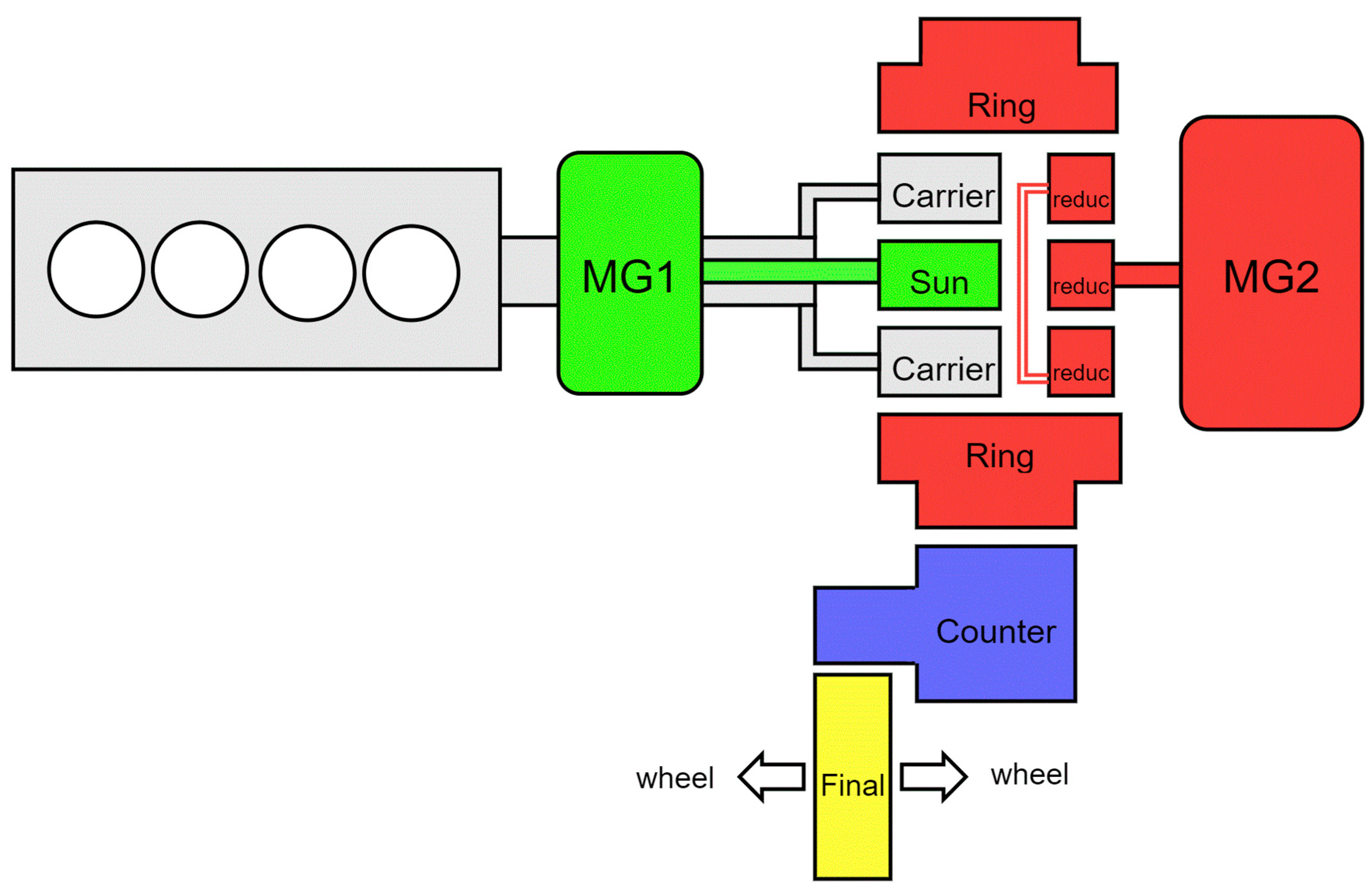
The Prius3′s powertrain configuration consists of three main powertrain components: Atkinson cycle engine, motor/generator 1 (MG1), and motor/generator 2 (MG2). MG1 is recognized as an electric generation motor, and MG2 is recognized as a propulsion motor. Power flows in these three components are integrated via a planetary gear set called a power-split device. Between the ring gear of the main planetary gear and MG2, Toyota added a speed-reduction gear, which is a planetary gear set with a fixed carrier to reduce MG2 speed and increase torque to be optimal for driving. The powertrain structure is shown in Figure 2. The engine is engaged with the carrier that holds all pinions inside the carrier case. MG1 and MG2 are mounted with the sun and ring gears, respectively.

The engine is considered as the primary power source for driving and battery recharging. Power from the engine is always split into two paths, sun and ring gear, via power-split device transmission. The engine power transmitted to the sun gear flows to MG1, which mainly generates engine power to electricity and distributes power to the battery, MG2, or auxiliary components, such as the air conditioner and pumps. MG1 also acts as a starter and engine-/vehicle-speed controller. The engine power transmitted to the ring gear flows directly to the wheel and/or to MG2, which acts as the main driving motor, regenerative braking generator, and driving-torque-assisting motor. In some situations, the MG2 is also used as a generator to absorb engine-power residue and store power in the battery. The concept of this hybrid configuration was to minimize poor engine-efficiency operation while providing a pleasant driving performance.

Due to the complexity of the operation of Prius3′s powertrain, torque transfer was analyzed in a free-body diagram to allow comprehensive visualization of powertrain activities, shown in Figure 3.

At the carrier, the engine exerts torque to the carrier, which creates the reaction torques on the sun gear (${\tau }_{C>S}$) and ring gear (${\tau }_{C>R}$). These reaction forces also represent the torque split from the engine being distributed to the sun and ring gear. The torque split to the sun gear is balanced with the electricity-generation torque from MG1. This MG1 generation torque also enables the engine torque to transfer to the ring and wheels. However, this hybrid system also utilizes MG1 as an engine-speed controller by operating MG1 in the motor mode. All the torque components from the powertrain are denoted in a positive direction. By applying Newton’s second law (∑τ = Iω) at the carrier and sun gear, the engine torque (${\tau }_{ice}$) and torque transferred from the engine to the sun (${\tau }_{C>S}$) can be expressed as Equations (5) and (6), respectively:

$${\tau }_{ice}={\dot{\omega }}_{ice}\left(I_{ice}+I_C\right)+{\tau }_{C>R}+{\tau }_{C>S},$$

(5)

$${\tau }_{C>S}={\dot{\omega }}_{MG1}\left(I_{MG1}+I_s\right)-{\tau }_{MG1}.$$

(6)

Assuming a steady-state torque split from the engine to the sun and ring gear, the torque transferred from engine to ring (${\tau }_{C>R})$ can be expressed as Equation (7):

$${\tau }_{C>R}=\frac{R}{\left(R+S\right)}{\tau }_{ice}=\frac{R}{S}{\tau }_{C>S}.$$

(7)

Equation (8) represents the engine torque and can be obtained by substituting Equations (6) and (7) in Equation (5). This equation indicates that engine torque is a product of both engine and MG1 motion:

$${\tau }_{ice}= {\dot{\omega }}_{ice}\left(I_{ice}+I_C\right)+\left(\frac{R+S}{S}\right)\left[{\dot{\omega }}_{MG1}\left(I_{MG1}+I_S\right)-{\tau }_{MG1}\right].$$

(8)

At the ring gear, the engine-torque split to the ring gear is combined with the torque from MG2. Between MG2 and ring gear, there is MG2 speed-reduction planetary gear of which the carrier is stationary; the gear ratio is expressed by $G_r$. Then, total powertrain propulsion torque is transferred to wheels passing through the counter gear and final gear. Gear ratios are denoted as $G_c$ and $G_f$. After applying ∑τ = Iω to the wheels, Equation (9) is yielded. To calculate wheel rotational speed $\left({\omega }_{wheel}\right)$, it is recommended to use MG2′s rotational speed, since MG2′s rotational speed sensor provides much higher precision than the vehicle-speed sensor does. The associated equation is expressed as Equation (10):

$$\begin{array}{c}\left(\frac{{\tau }_{MG2}}{(G_r·G_c·G_f)}\right)+\left[\left(\frac{R}{R+S}\right){\tau }_{ice}·\frac{1}{G_c·G_f}\right]-{\tau }_{drv\_resist}-{\tau }_{brake,mech}= \\ {\dot{\omega }}_{wh} \{\frac{I_R}{(G_c·G_f)}+\frac{I_{MG2}}{(G_r·G_c·G_f)}+I_{wh}\},\end{array}$$

(9)

$${\omega }_{wh}=\left(G_r·G_c·G_f\right){\omega }_{MG2}.$$

(10)

Thus, when mechanical braking is not being applied, powertrain driving torque (${\tau }_{PTdrv}$) must satisfy the required torque for driving acceleration and the required torque to overcome all driving resistances: rolling resistance, aerodynamic drag, road grade resistance, and other powertrain losses. This term aims to represent vehicle driving activity and is expressed by ${\tau }_{drv\_resist}$. Driving-torque and -power ($P_{PTdrv}$) equations are expressed as Equations (11) and (12), respectively:

$${\tau }_{PTdrv}\cong {\tau }_{dr{v}_{resist}}\cong \left(\frac{{\tau }_{MG2}}{(G_r·G_c·G_f)}\right)+\left[\left(\frac{R}{R+S}\right){\tau }_{ice}\times \frac{1}{G_c·G_f}\right]-{\dot{\omega }}_{wh} \left\{\frac{I_R}{\left(G_c·G_f\right)}+\frac{I_{MG2}}{(G_r·G_c·G_f)}+I_{wh}\right\},$$

(11)

$$P_{PTdrv}={\tau }_{PTdrv}{\omega }_{MG2@Wh}$$

(12)

$P_{PTdrv}$, calculated by the Prius3′s powertrain dynamic equation, is used in VSP coefficient calibration and optimization.

2.3. Vehicle-Driving-Power Equation Formulation and Coefficient Calibration

This section presents a methodology for driving-power equation formulation and Prius3 coefficient calibration. First, the stepwise algorithm was applied to analyze the significance of each term and select the significant terms into the final driving-power equation. This step aimed to simplify the equation, and minimize the complexity of data acquisition and model updating. Then, coefficients and specific vehicle constants were calibrated on the basis of the multiple regression method as expressed in Equation (13):

$$Y ={\beta }_1{x}_1+{\beta }_2{x}_2+{\beta }_3{x}_3+\dots +{\beta }_n{x}_n+ϵ.$$

(13)

To investigate the significance of the equation terms, the forward–backward stepwise algorithm was implemented with the multiple regression process. This algorithm automatically eliminates and selects variables in the model on the basis of quality of fitness. The process begins with regressing each variable term ($x_i$) with the independent term ($Y$). The term that provides the lowest p-value, which must be lower than a specified entrance tolerance, was initially included into the equation. Next, multiple regression was applied to test the next candidate term. The term was selected into the equation by the same p-value criteria; however, the removal process also took place at this stage. In the removal process, if any terms that were included into the model were found to have a p-value larger than the removal-tolerance level, the term that contained the largest p-value was removed from the model. In this study, the entrance tolerance and the removal tolerance were set at a p-value smaller than 0.1 and larger than 0.15, respectively.

According to the equation terms frequently used in the literature in Table 1, this study arranged the equation terms into two different combinations described as Independent Variables (Indt var.) 1 and 2 in

Table 2. Independent-variable (Indt var.) sets for stepwise variation process.

Terms	Coefficients		$\mathbf{Indt}\mathbf{var}.1\left({\mathbf{X}}_1\right)$	$\mathbf{Indt}\mathbf{var}.2\left({\mathbf{X}}_2\right)$
Acceleration	${\beta }_{acc}$	m	$v_{veh}{a}_{veh}$	$v_{veh}{a}_{veh}$
Road grade	${\beta }_{grd}$	mg	$v_{veh}sin\theta$	$v_{veh}sin\theta$
Aerodynamic drag	${\beta }_{aero}$	$\frac{1}{2}{\rho }_{air}A{C}_d$	$v_{veh}{\left(v_{veh}-v_{wind}\right)}^2$	$v_{veh}{\left(v_{veh}-v_{wind}\right)}^2$
Rolling resistance and road friction	${\beta }_{roll1}$	$mg{C}_r{C}_1$	-	$v_{veh}{}^{2}cos\theta$
	${\beta }_{roll2}$	$mg{C}_r{C}_2$	$v_{veh}cos\mathsf{\theta }$	$v_{veh}cos\theta$
Other road loads	${\beta }_{e1}$	-	-	$v_{veh}{}^3$
	${\beta }_{e2}$	-	-	$v_{veh}{}^2$
	${\beta }_{e3}$	-	-	$v_{veh}$

. Independent Variable 1 represents the basic driving-power equation that includes all conventional contribution terms. Independent Variable 2 represents the detailed estimation equation, which includes all contribution terms existing in the literature review. In the coefficients column, the left column describes the signs denoted for each coefficient term that is calibrated by the multiple regression method. The right column shows the definition of the derived coefficients from the theoretical conservative energy equation. The dependent variable ($Y_1$) was $P_{PTdrv}$. Data in this process excluded data from when reverse driving and mechanical braking were actuated. After the outliner was removed, the dataset obtained more than 98,000 samples. The best-candidate equation was selected on the basis of R-square and error-residue distribution.

3. Results and Discussion

Table 3. Coefficient calibration for Prius3 driving-power equations.

Equations	Coefficient		SD	p-Value	R2
Indt var. 1 (${\mathit{X}}_{\mathbf{1}}$)	${\beta }_{acc}$	1624	1.159	$\cong 0$	0.96 (<50 kW) 0.96 (≥50 kW)
	${\beta }_{grd}$	18,670	31.80	$\cong 0$
	${\beta }_{aero}$	0.912	0.0011	$\cong 0$
	${\beta }_{roll2}$	206.41	1.597	$\cong 0$
	$DrvP{w}_{Indt var1}={\beta }_{acc}{v}_{veh}{a}_{veh}+{\beta }_{grd}{v}_{veh}sin\theta +{\beta }_{aero}{v}_{veh}{\left(v_{veh}-v_{wind}\right)}^2$ $+{\beta }_{roll}{v}_{veh}cos\theta$
Indt var. 2 (${\mathit{X}}_{\mathbf{2}}$)	${\beta }_{acc}$	1624	1.175	$\cong 0$	0.96 (<50 kW) 0.96 (≥50 kW)
	${\beta }_{grd}$	18,900	36.87	$\cong 0$
	${\beta }_{aero}$	0.2567	0.0054	$\cong 0$
	${\beta }_{roll1}$	1163	284.5	4.379 × 10−5
	${\beta }_{roll2}$	12320	6068	0.0424
	${\beta }_{e1}$	0.3362	0.0094	1.373 × 10−279
	${\beta }_{e2}$	−1163	284.4	4.338 × 10−5
	${\beta }_{e3}$	−1.214	6068	0.0454
	$DrvP{w}_{Indt var2}= {\beta }_{acc}{v}_{veh}{a}_{veh}+{\beta }_{grd}{v}_{veh}sin\theta +{\beta }_{aero}{v}_{veh}{\left(v_{veh}-v_{wind}\right)}^2$ $+{\beta }_{roll1}{v}_{veh}{}^{2}cos\mathsf{\theta }+{\beta }_{roll2}{v}_{veh}cos\mathsf{\theta }+{\beta }_{e1}{v}_{veh}{}^3+{\beta }_{e2}{v}_{veh}{}^2+{\beta }_{e3}{v}_{veh}$
VSP LDV 1999	$VS{P}_{LDV1999} \left[watt\right]=m\times v_{veh}\left[1.1 a_{veh} + 9.81\times sin\left({tan}^{-1}\left(\frac{h}{l}\right)\right)+0.132\right]$ $+ m\times 0.000302v_{veh}{}^3$				0.93 (<50 kW) 0.79 (≥50 kW)
VSP Prius3Spec	$VS{P}_{Prius3}\left[watt\right]=m\times v_{veh}\left[a_{veh}\left(1+{\epsilon }_i\right)+g\times sin\left({tan}^{-1}\left(\frac{h}{l}\right)\right)+g\times C_{roll}\right]$ $+\frac{1}{2}{\rho }_{air}{C}_{drag}A\times v_{veh}{\left(v_{veh}-v_{wind}\right)}^2$				0.94 (<50 kW) 0.78 (≥50 kW)

shows the coefficient-calibration results found on the basis of $P_{PTdrv}$ data. Results include the equations’ coefficients, standard deviation (SD), and the p-value obtained from the two different sets of independent-variable equations (Indt var. 1 and 2). According to the results, p-values indicate that acceleration, road-grade climbing, and rolling resistance were the primary contributors to vehicle power utilization. This table also shows the comparison of the goodness of fit between Indt var. 1 and d 2′s coefficients, the conventional VSP for LDV’s coefficients (VSP LDV1999), and the conventional VSP with Prius3′s specific parameters’ coefficients (VSP Prius3Spec) by using R-square. R-square results were separated into light-load-driving (<50 kW) and heavy-load-driving (≥50 kW) ranges to clarify the prediction accuracy of the four equations.

In the light-load-driving range, all four equations provided a high R-square at a satisfying level. R-squares associated with Indt var. 1 and 2 equations were found at 0.96, while the R-squares of VSP LDV 1999 and VSP Prius3Spec were found at 0.93 and 0.94, respectively. Nevertheless, this study discovered that the conventional VSP equation of VSP LDV1999 and VSP Prius3Spec provided significantly lower R-squares once they were under the heavy-driving load. The R-squares of VSP LDV 1999 and VSP Prius3Spec were reduced to 0.79 and 0.78, respectively, while the R-squares of Indt var. 1 and 2 remained at 0.96 throughout the light- and heavy-load-driving ranges. In other words, the new coefficient sets for Prius3 obtained in Indt var. 1 and 2 improved driving-power prediction during heavy-load driving by 21% to 22% compared to the conventional VSP equations.

Since Indt var. 1 and 2 provided R-squares at the same level during both light- and heavy-load driving, this study selected the Indt var. 1 equation to represent the Prius’ driving-power estimation equation for further analysis, called $DrvP{w}_{Prius3}$. Furthermore, Indt var. 1 seemed to provide a good balance between prediction accuracy and calculation complexity. The newly calibrated driving-power equation is expressed as Equation (14). To some extent, results indicated that applying complex rolling-resistance terms $mgcos\theta C_r(C_1{v}_{veh}{}^2$+ $C_2{v}_{veh})$, and the other road-load term, ${\beta }_1{v}_{veh}{}^3+{\beta }_2{v}_{veh}{}^2+{\beta }_3{v}_{veh}$, included in Indt var. 2, did not seem to provide significant prediction improvement compared to Indt var. 1:

$$\begin{array}{c}DrvP{w}_{Prius3}=0.9963 m\times v_{veh}\times a_{veh}+1.168mg\times v_{veh}sin\theta +\\ 1.523 {\rho }_{air}{v}_{veh}{\left(v_{veh}-v_{wind}\right)}^2+0.0129 mg\times v_{veh}cos\mathsf{\theta }.\end{array}$$

(14)

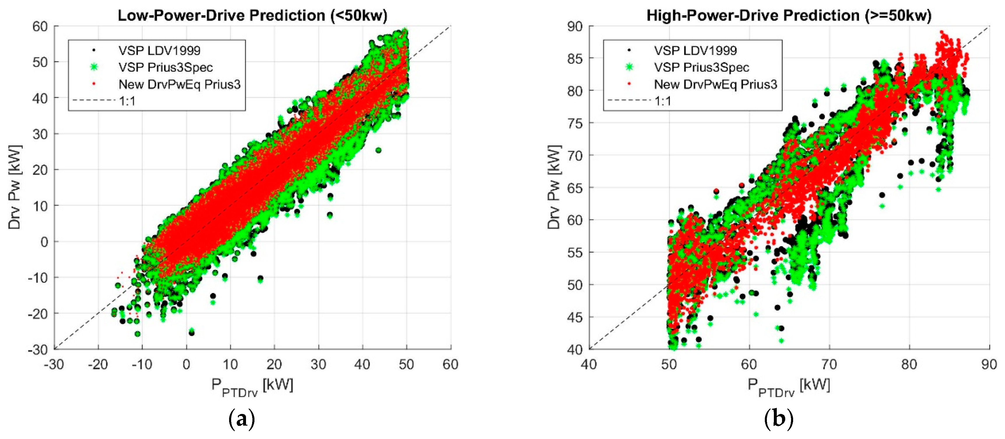
Figure 4 shows the validation results of the three driving-power estimation equations: $DrvP{w}_{Prius3}$, VSP Prius3Spec, and VSP LDV 1999, as compared to $P_{PTdrv}$. The validation results are from two different driving ranges: (a) light-load driving, in which driving power was less than 50 kW; and (b) heavy-load driving, in which the driving power was equal to or greater than 0 kW. Data incorporated in this analysis were data that had prediction error within the 95% confidential interval. The prediction error was calculated by the residue between prediction results and $P_{PTdrv}$.

In the light-load-driving condition, the data cloud from all three equations of VSP LDV 1999, VSP Prius3Spec, and ${\mathrm{DrvPw}}_{\mathrm{Prius}3}$ showed high correlation with $P_{PTdrv}$. The data clouds were densely aligned on the 1:1 diagonal line. VSP LDV 1999 and VSP Prius3Spec data showed similar alignment while $DrvP{w}_{Prius3}$ provided slightly less scattering and more symmetric results around the 1:1 line.

During heavy-load driving, these driving conditions were found in several driving scenarios, such as high-speed driving, aggressive driving, steep road gradient, strong head wind, or heavy cargo load. Even though these data do not represent typical driving situations in some countries or regions, heavy-load-driving conditions are the major factors that cause vehicles’ energy consumption and emissions to dramatically increase. Results from Figure 4b illustrate that, during heavy-load driving, $DrvP{w}_{Prius3}$ provided more critically predictable results compared to both the VSP LDV 1999 and VSP Prius3Spec equations. Results from VSP LDV 1999 and VSP Prius3Spec showed significant discrepancy from the main diagonal line when compared to $DrvP{w}_{Prius3}$.

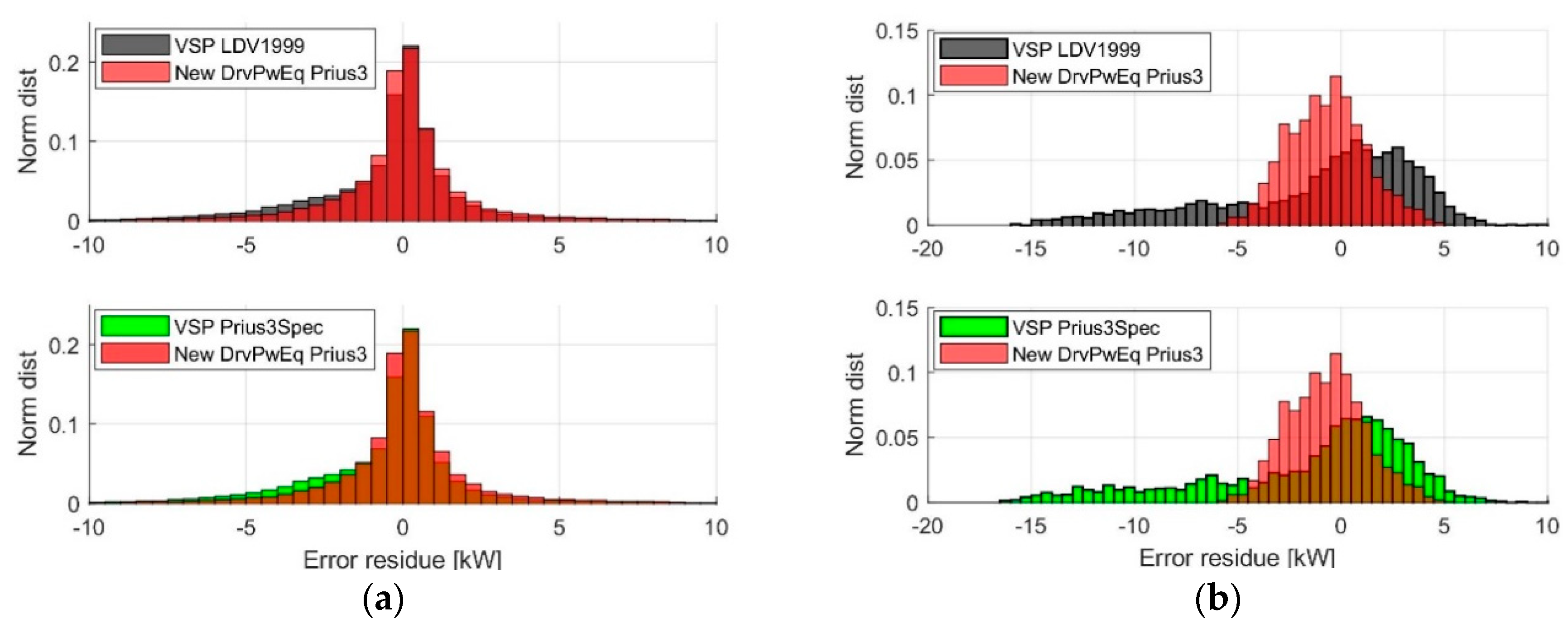
Due to the large size of the database plotted on Figure 4, it was difficult to distinguish the data-alignment concentration in the three datasets. Thus, Figure 5a,b presents the distributions of prediction-error residue of the three different driving-power estimation methods: $DrvP{w}_{Prius3}$, VSP Prius3Spec, and VSP LDV 1999, separated into light- and heavy-load-driving ranges. Error residues were computed on the basis of $P_{PTdrv}.$

In the light-load-driving condition, the error distributions of VSP LDV 1999, VSP Prius3Spec, and $DrvP{w}_{Prius3}$ presented normally shaped distributions. Nevertheless, the error distributions of VSP LDV 1999 and VSP Prius3Spec tended to shift to the left, which means that these conventional equations provided slightly underpredicted results. In the heavy-load-driving condition, $DrvP{w}_{Prius3}$ produced the prediction error in normally shaped distribution, and the peak was located at 0 kW. Maximal error was found at ±5 kW. On the other hand, the error distributions of VSP LDV 1999 and VSP Prius3Spec covered the range of −15 to 10 kW, which was 2.5-fold wider than the error range of $DrvP{w}_{Prius3}$. Moreover, the distribution peaks of VSP LDV 1999 and VSP Prius3Spec slightly shifted to the right and were located at approximately 1.25 kW.

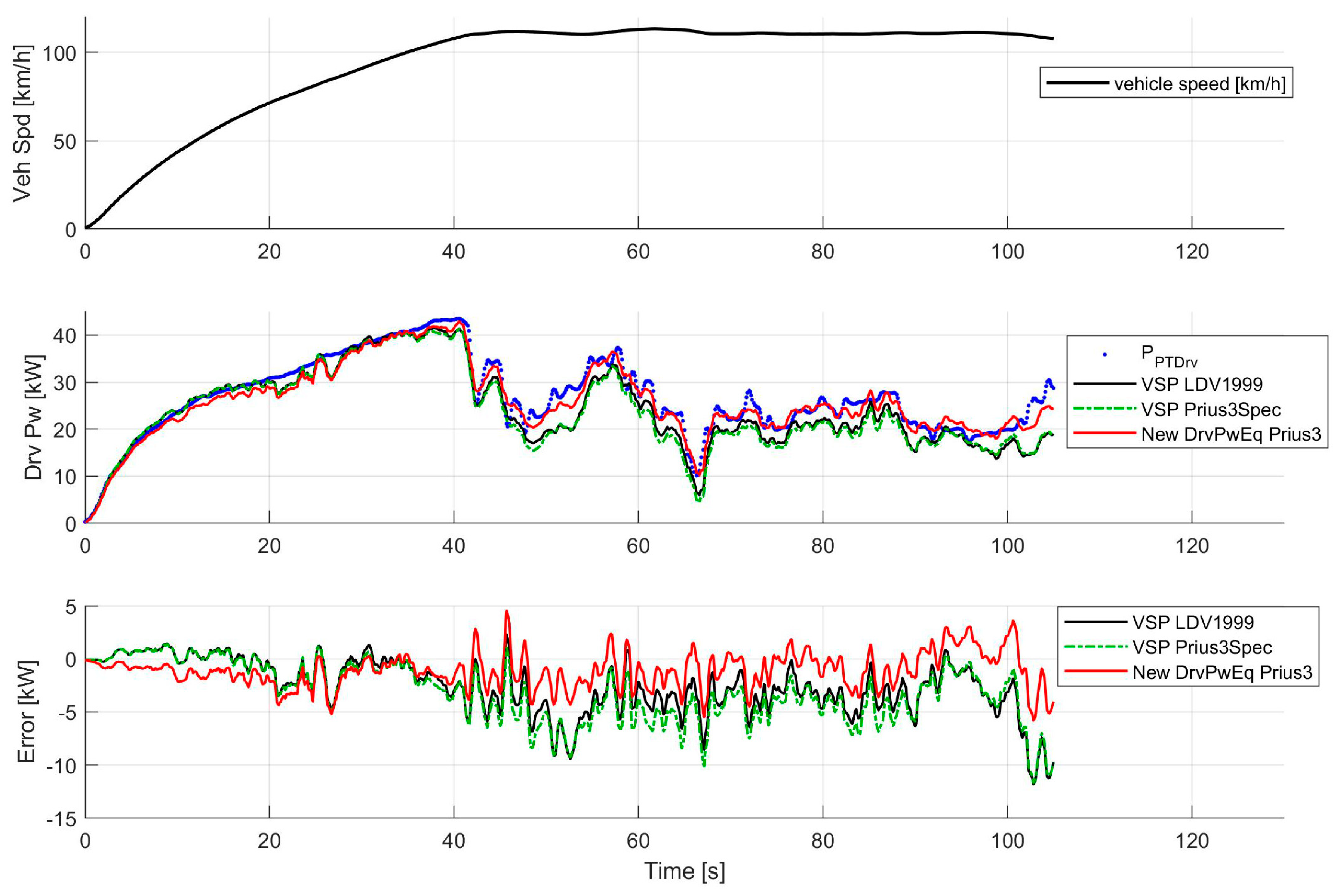
Furthermore, this study performed validation by analyzing prediction results and error analysis on the basis of actual driving datasets. Figure 6 shows the obtained results from naturalistic acceleration and a high-speed cruising speed profile. This dataset represents the light-load-driving condition in which driving-power utilization was less than 50 kW. Figure 6 is divided into three parts, namely, vehicle-speed profile, comparison between predicted driving powers to $P_{PTdrv}$, and prediction-error residues. At the initial naturalistic acceleration duration, all three equations provided slightly underpredicted results. However, the power-utilization trajectories still captured the major driving-power utilization trend. Once speed became constant at around 110 km/h, $DrvP{w}_{Prius3}$ seemed to provide the best prediction results. There were some small fluctuations at some local spikes, but it still captured the tendency well. VSP LDV 1999 and Prius3Spec tended to provide underpredicted results at the high-speed- and light-load-driving conditions. For error-residue analysis, results showed that $DrvP{w}_{Prius3}$ produced an error fluctuating at around 0 kW, while VSP LDV 1999 and Prius3Spec produced an error fluctuating approximately at −3 kW, which accounts for 15% of driving-power level.

Figure 7 presents the prediction results in the heavy-load-driving condition during the maximal-acceleration test. For Prius3, 0 to 60 km/h is the speed range in which the vehicle can provide the most powerful acceleration. As a result, driving power escalated sharply at the beginning. At this section, overshoots were found from the VSP LDV 1999 and Prius3Spec prediction results. These conventional equations provided similar prediction results, which were underpredicted during the first half of the acceleration. As vehicle speed increased, results became more underpredicted. Between the three equations, $DrvP{w}_{Prius3}$ was potentially the most accurate and reliable prediction. Through $DrvP{w}_{Prius3}$ produced some error, it fluctuated around the zero-error line.

This study also analyzed the impact of vehicle speed on the magnitude of prediction errors, discovering that the error generated by VSP LDV 1999 and VSP Prius3Spec is not only subject to the driving-power level, but also driving speed. When driving speed increased, VSP LDV 1999 and VSP Prius3Spec were prone to produce exponentially underpredicted results, as seen in the two top charts in Figure 8. Error residues started to deviate from the zero error line after vehicle speed reached 80 km/h. The data show that the prediction error of both conventional could can increase up to −20 kW. Unlike $DrvP{w}_{Prius3}$, there was no significant deviation found from the driving-power prediction results shown in Figure 8 in the third chart from the top. The error was populated on the zero-error line from zero to maximal speed of 160 km/h. Furthermore, the width of the error cloud was also significantly reduced compared to both the VSP LDV 1999 and VSP Prius3Spec results.

In the bottom chart in Figure 8 is typical driving-speed distribution, recorded in Nagoya, Japan. The experiment was conducted for city (Sakae area) and highway (Tomei expressway from Hongo and Komaki) driving. The data showed that driving speed in city traffic was between 0 and 30 km/h, while top speed was recorded at roughly 55 km/h. On the highway, vehicle driving-speed range increased to between 80 and 100 km/h.

Results from Figure 8 indicated that, in the case of city driving, the three equations were appropriate for driving-power estimation. $DrvP{w}_{Prius3}$ only provided slightly higher prediction accuracy. Nevertheless, in the case of highway driving or higher-speed driving conditions, estimating driving power with VSP LDV 1999 and VSP Prius3Spec may cause a significant driving-power prediction error of up to −20 kW.

This study also provides an analysis on the cause of the error. Figure 9 shows the relationship between total prediction error and power-utilization magnitude of aerodynamics and rolling-resistance terms. Strong correlation implies that the particular term had significant influence on prediction-error occurrence, which was only found in aerodynamics and rolling-resistance terms. Results showed that the aerodynamics and rolling-resistance terms were the primary factors that contributed to the underpredicted error of VSP LDV 1999 and VSP Prius3. As the magnitude of the power utilizations of these two terms became larger, it resulted in the exponential growth of the total prediction error.

For the aerodynamics term, the prediction by VSP LDV 1999 and VSP Prius3 showed error deviation after the magnitude became larger than 15 kW. The possible maximal error caused by this term was found to be up to 15 kW. On the other hand, $DrvP{w}_{Prius3}$ was prone to mitigating the underprediction problems of the conventional methods. Prediction results only showed slight deviation after magnitude reached 23 kW. Maximal error was also effectively reduced to 3 kW.

The power utilization of the rolling-resistance term was found in the range of 0 to 8 kW, which was less than that of the aerodynamics term. The prediction by VSP LDV 1999 and VSP Prius3 showed a similar deviation trajectory. The error began to deviate at magnitudes larger than 5 kW. $DrvP{w}_{Prius3}$ significantly reduced the error caused by this term; however, it began to deviate after 7 kW.

Acceleration and road-grade terms could be considered as minor error contributors compared to the aerodynamics and rolling-resistance terms. No significant correlation was found between error and magnitude, which implies that the road-grade terms were not major factors that caused the driving-power prediction error.

For further improvement of the proposed $DrvP{w}_{Prius3}$ equation formulated by Indt var. 1, this study found that the trajectory of the error curve established a polynomial trend that could be properly fitted by a quadratic function of vehicle speed. In the case that high accuracy of driving-power estimation is required, this study recommends using the $DrvP{w}_{Prius3}$ equation formulated by Indt var. 2, which contains the quadratic function of the vehicle-speed terms. This study also confirmed that the $DrvP{w}_{Prius3}$ equation formulated by Indt var. 2 is capable of suppressing the error caused by the aerodynamics and rolling-resistance terms. However, higher accuracy also comes with higher calculation complexity. The best practice is to select the equation that provides acceptable accuracy in a particular driving condition.

Additionally, this study provides a summary of the impact of energy utilization classified by each acceleration and driving-resistance term based on Nagoya’s city- and highway-driving conditions. Figure 10 shows the comparison of Prius3′s driving energy utilization between city and highway driving. Data were classified into each contributor term: acceleration, road grade, aerodynamic, and rolling resistance, which were estimated by the terms in Equation (14). In the city, more than 70% of energy was utilized for acceleration, which mostly took place during a stop-and-go situation. Approximately 20% of the energy was used to overcome rolling resistance. The effect of the road-grade and aerodynamic terms was comparatively small at 6% and 2%, respectively. On the other hand, energy utilization during highway driving showed that the proportion of the utilized energy by the acceleration term was decreased by half, while the effect of the road grade and aerodynamics increased 4- and 10-fold, respectively. In addition, only the acceleration and road-grade terms, which are surplus to the aerodynamic and rolling-resistance terms, could be recuperated during regenerative braking.

According to the impact of the energy utilization classified by each term, as shown in Figure 10, it can be concluded that, during city driving, it is recommended to ensure the accuracy of the acceleration and rolling-resistance terms. However, during highway driving, the contribution of all four terms fairly shares this significance. Thus, all coefficients in front of the four equation terms should be deliberately calibrated for accuracy of driving-power prediction.

More importantly, this analysis also indicates two different vehicle driving-power calculation approaches, which are a direct calculation of powertrain propulsion output power and vehicle-specific power approaches. These two approaches require different sets of input parameters. One directly calculates driving power from the hybrid powertrain ($P_{PTdrv}$), and requires ${\omega }_{MG1}$, ${\tau }_{MG1}$, ${\omega }_{MG2}$, ${\tau }_{MG2}$, and ${\omega }_{Ice}$ as input parameters. The other calculates driving power from the vehicle’s external observable parameters (VSP and $DrvP{w}_{Prius3}$), and requires $v_{veh}$, $v_{wind},a_{veh}, and \theta$ as input parameters. However, these two approaches established a significantly high correlation degree, thus confirming that these two calculation approaches are valid for hybrid-vehicle driving-power estimation. Moreover, it is reasonable to conclude that the driving-power equation-coefficient calibration method proposed in this study is capable of providing an appropriate set of coefficients for any interested vehicle model or fleet.

4. Conclusions

Vehicle driving power is one of the most substantial parameters in vehicle energy-consumption modeling and analysis. This study developed a vehicle driving-power estimation equation for hybrid vehicles and proposed a procedure to calibrate an optimal set of vehicle-specific coefficients for acceleration, road-grade, rolling-resistance, and aerodynamics terms.

The approach utilized the power-split hybrid powertrain’s accessible OBD dataset and its dynamic model to estimate the total propulsion power of the power-split hybrid powertrain in Prius3. Then, propulsion power was utilized as a key parameter for driving-power equation development and vehicle-specific coefficient calibration. The stepwise algorithm was introduced to determine the significance of each equation term. Then, this study implemented the multiple regression method to calibrate a set of coefficients that were optimal for a particular vehicle model or fleet.

Results showed that conventional driving-power equations VSP LDV 1999 and VSP Prius3Spec suffer from prediction error, particularly under heavy-load- and high-speed-driving conditions. During heavy-load driving, when power was greater than 50 kW, the correlation between VSP LDV 1999 and VSP Prius3Spec with $P_{PT\_drv}$ was found at an R-square of 0.79 and 0.78, respectively. During light-load driving, VSP LDV 1999 and VSP Prius3Spec also tended to deliver slightly underpredicted results. Furthermore, at driving speeds higher than 80 km/h, VSP LDV 1999 and VSP Prius3Spec also caused underestimated prediction error. As speed increased, the error became more severe; maximal error ranged up to −20 kW. This error was primarily generated by the aerodynamics and rolling-resistance terms.

However, the new driving-power equation, $DrvP{w}_{Prius3}$, dramatically improved estimation accuracy over the two conventional VSP equations. It provided a consistent R-square of 0.96 in both light- and heavy-load-driving conditions. The error also established normally shaped distributions, which showed better reliability for prediction results. Moreover, $DrvP{w}_{Prius3}$ was also capable of suppressing error during high-speed driving, and significantly reduced the error generated by the aerodynamics and rolling-resistance terms. According to analysis, $DrvP{w}_{Prius3}$ is appropriate for application to all driving conditions, since it consistently provided a low prediction error from light- to heavy-driving power, and low- to maximal-speed driving compared to VSP LDV 1999 and VSP Prius3Spec.

For such an application, this study recommends that the coefficients be calibrated for the specifically studied vehicles or fleet, whether in city or highway driving. The reason is that, in city driving, the rolling-resistance term dominates 21% of total energy consumption. In highway driving, the aerodynamics and rolling-resistance terms dominate 23% and 24%, respectively, of energy consumption. Particularly during heavy-load driving, $DrvP{w}_{Prius3}$ can provide much more accurate prediction.

Lastly, results in this study showed that both of the approaches used to establish the $P_{PTdrv}$ and $DrvP{w}_{Prius3}$ equations are rational for power-split hybrid-vehicle driving-power estimation. For the coefficient-calibration part, the stepwise and multiple regression method introduced in this study was capable of providing an appropriate set of coefficients that were optimal for a specific vehicle model or fleet. This coefficient-calibration method could be applied through all kinds of powertrains and vehicle types as long as driving power can be measured or estimated from the vehicles.