Numerical Investigation on the Flow Characteristics in a 17 × 17 Full-Scale Fuel Assembly

Abstract

In a previous study, several computational fluid dynamics (CFD) simulations of fuel assembly thermal-hydraulic problems were presented that contained fewer fuel rods, such as 3 × 3 and 5 × 5, due to limited computer capacity. However, a typical AFA-3G fuel assembly consists of 17 × 17 rods. The pressure drop levels and flow details in the whole fuel assembly, and even in the pressurized water reactor (PWR), are not available. Hence, an appropriate CFD method for a full-scale 17 × 17 fuel assembly was the focus of this study. The spacer grids with mixing vanes, springs, and dimples were considered. The polyhedral and extruded mesh was generated using Star-CCM+ software and the total mesh number was about 200 million. The axial and lateral velocity distribution in the sub-channels was investigated. The pressure distribution downstream of different spacer grids were also obtained. As a result, an appropriate method for full-scale rod bundle simulations was obtained. The CFD analysis of thermal-hydraulic problems in a reactor coolant system can be widely conducted by using real-size fuel assembly models.

1. Introduction

Currently, reactor fuels are developing toward using high power and having long cycles. It is necessary to improve the safety analysis of the heat transfer on fuel rod surfaces and increase the power of the bundle. To enhance the heat transfer performance, the main aim is to improve the fuel assembly structure design. The spacer grid is the only device installed in the heating section of the fuel assembly. Hence, changing the spacer grid configuration and the shape of the mixing vanes on the grid is vital to improving the heat transfer performance of the fuel assembly.

Starting from the late 1990s, researchers began to study the flow characteristics of the rod bundle channel through a spacer grid in Particle Image Velocimetry (PIV) and Laser Doppler Velocimetry (LDV) experimental studies. McClusky [1] used PIV to measure the lateral velocity of the typical sub-channel with the mixing vanes in the fuel assembly. The transverse kinetic energy, the maximum lateral velocity, the vortex center position, and the circumferential velocity distribution were obtained. Holloway [2,3] carried out single-phase flow and heat transfer experiments with 5 × 5 rod bundles. They measured the pressure loss of all grid sections and rod bundles, as well as the change of the Nu number along and around the rod. They calculated the pressure loss coefficient caused by the mixing vanes and fitted the Nu number change of the rod bundles under the two working conditions of Re = 28,000 and 42,000. Conner [4] measured the lateral velocity distribution of a rod bundle cross-section using PIV technology. They also measured the average heat transfer coefficient, circumferential heat transfer coefficient, and fully developed heat transfer coefficient using the positioning grid rod bundle test section, similar to Holloway.

Compared with the cost of experimentation, most nuclear energy manufacturers use numerical methods to analyze the results and modify the design. A large number of numerical results have also been verified using experimental data. Karoutas [5] studied the mixing characteristics of mixing vanes and compared the difference of axial and lateral velocities between LDV measurements and computational fluid dynamics (CFD) simulations. The results showed that the mixing phenomena in the experiments and simulations were in agreement. Seok [6] used two-dimensional LDV to study the flow field structure of a 5 × 5 rod bundle and investigated the typical split-type and swirl-type mixing vanes. The split type had no significant swirling flow and lateral flow while there was a relatively small lateral flow in the swirl type. Sang [7] studied the mixing effect of tandem arrangement vane (TAV) mixing vanes and compared the results of LDV and CFD. The results showed the applicability of CFD to design fuel rod spacer grids. Conner [8] used PIV to carry out experimental tests. The results showed that the geometrical shape and axial velocity components of mixing vanes can effectively improve the secondary flow and heat transfer performance. The test technology was based on the benchmark data of CFD and pressurized water reactor (PWR) bundles.

At the same time, CFD was also widely used to study refined turbulence phenomenon to provide a more detailed geometric optimization of a spacer grid. Wang [9] used CFD to simulate three spacer grids with different kinds of mixing vanes: split vane, swirl vane, and twisted vane. The results predicted that the split vane had better coolant mixing characteristics. Cui [10] used CFD to study a three-dimensional split-vane spacer grid. The turbulence models they used to calculate were the standard k-ε, standard k-ω, and Reynolds stress model. The study showed that the analysis and prediction of the standard k-ε turbulence model is better than standard k-ω and RSM. Holloway’s [11] research showed the importance of choosing appropriate turbulence models and the shear stress transport (SST) k-ω turbulence model obtained a successful simulation of a low Reynolds number area near the wall. Nematollahi [12] evaluated the effects of flow and heat transfer intensity with different mixing vanes on spacer grids. The vanes were divided into split vane, ripped open shape, trumpet shape, and split trumpet shape. The standard k-ε turbulence model was used and the results showed that the heat transfer coefficient was increased by 14% with split trumpet vanes. Yan [13] investigated the heat transfer and turbulence phenomena in four groups of fuel assemblies using large eddy simulation (LES) and unsteady Reynolds-averaged Navier–Stokes (URANS) simulation. The results showed that the average wall shear stress and the friction resistance both increased with the decrease of the rolling period. The URANS turbulence results were similar to the experimental results. Liu [14] further utilized different turbulence models and a near-wall mesh treatment. Through the comparison with experimental results, it was found that the flow field and heat transfer distribution were effectively obtained by using a realizable k-ε model and a near-wall treatment. Ikeno [15] used the LES method to simulate the flow in fuel rods using three different fuel rod bundle distance ratios. With the increase of the bundle distance ratio, the LES turbulence model can accurately simulate the flow phenomena in the fuel but heat transfer was not included in the study. Bae [16] investigated the friction coefficient of fuel rods using an SST k-ω turbulence model. The triangular and quadrangular arrangements were used to measure the shear stress distribution on the fuel rods. Therefore, it can be seen from the above literature that CFD will be effective in the design and research of nuclear energy components.

However, the current results were only for small-scale or simplified components and the calculation results for full-scale fuel components were scarce. The flow field distribution in the whole assembly and the secondary flow vortices generated by the spacer grid were not fully assessed. Numerical simulation research for the whole fuel assembly and even the whole PWR will allow for the pressure distribution and resistance levels to be evaluated during reactor operations, while also obtaining flow details that were not available in the experiments. In this study, a CFD simulation for the full-scale 17 × 17 fuel assembly was the focus. The polyhedral and extruded mesh was generated using Star-CCM+ 13.02 software and the total mesh number was about 200 million. The lateral velocity distribution and pressure drop in the full-scale fuel assembly sub-channels was investigated. A CFD simulation scheme to achieve a complete full fuel assembly simulation was obtained that will be a prerequisite for a refined numerical simulation of the nuclear reactor’s thermal hydraulics.

2. Mathematical Model

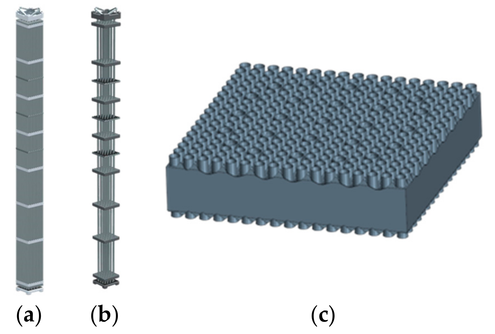
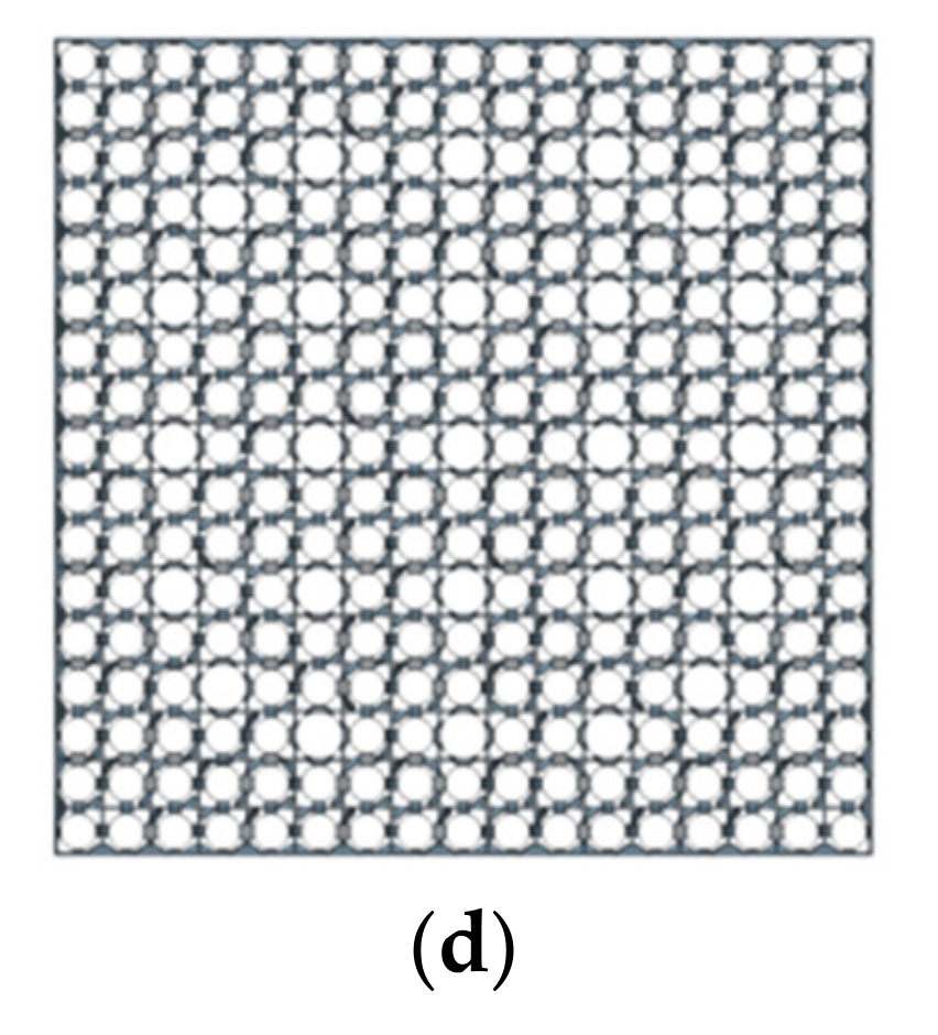
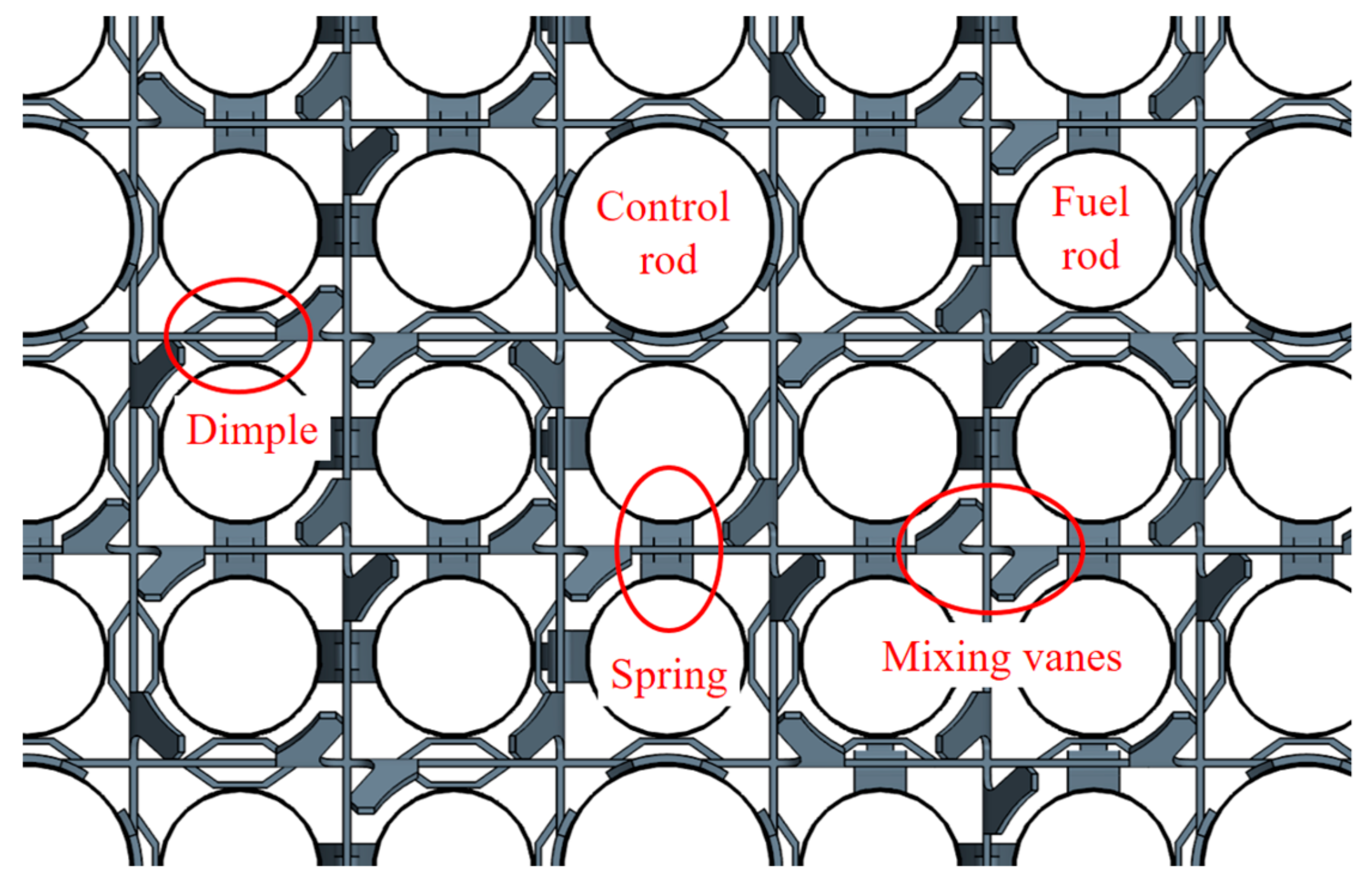
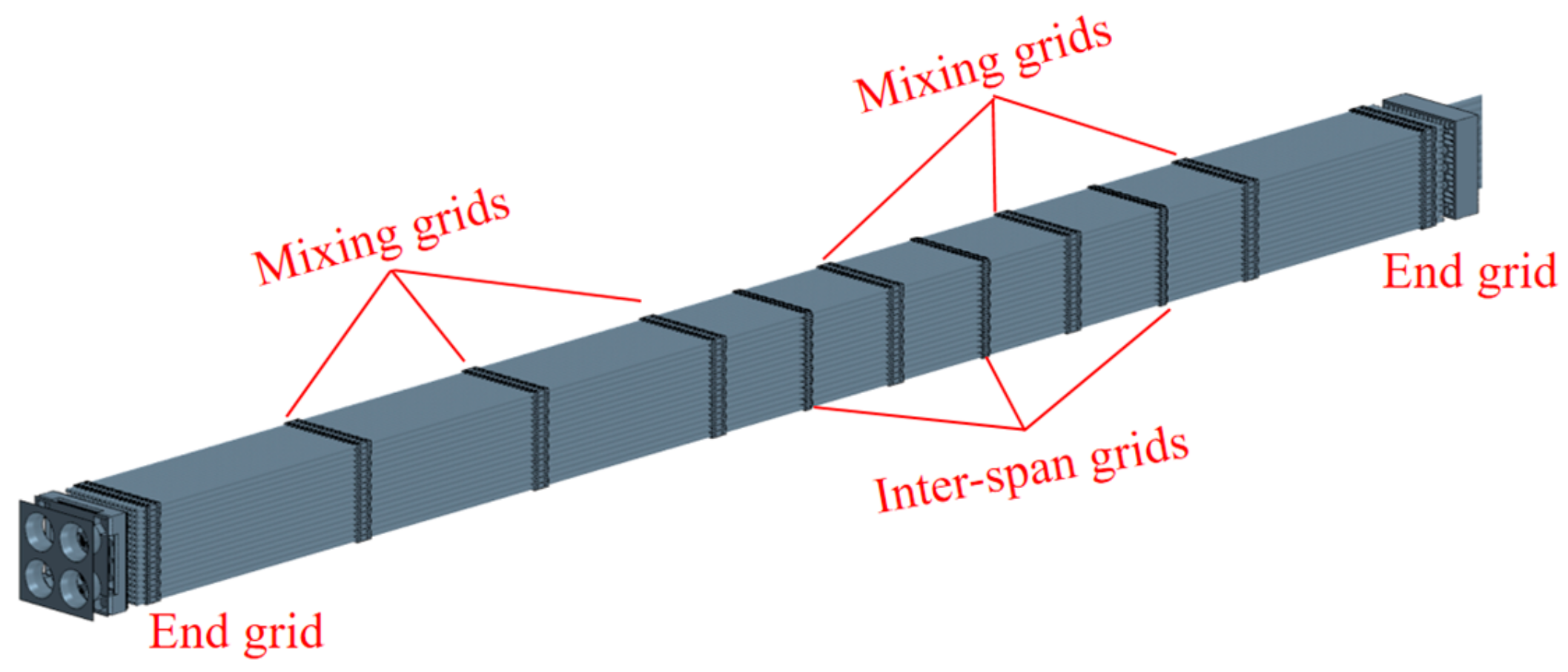
A 3D CFD methodology was developed in this paper to investigate the thermal-hydraulic characteristics in a rod bundle with split-vane pair grids. The RANS equations with the SST k–ω turbulence model were adopted after being verified by experiments. The mathematical model can be described as follows:

Continuity equation:

$$\frac{\partial }{\partial x_i}\left(\rho u_i\right)=0.$$

(1)

ρ is the density and u_i is the velocity vector in i direction.

Momentum equation:

$$\frac{\partial }{\partial x_i}\left(\rho u_i{u}_j\right)=-\frac{\partial p}{\partial x_i}+\frac{\partial {\tau }_{ij}}{\partial x_j}+\rho g_i,$$

(2)

τ is the shear stress tensor and is defined by

$${\tau }_{ij}={\mu }^{*}\frac{\partial u_i}{\partial x_j};{\mu }^{*}=\mu +{\mu }_t.$$

(3)

μ is the viscosity and μ_t is the turbulence induced viscosity.

Energy equation:

$$\frac{\partial }{\partial x_i}\left(\rho Cp{u}_{i}T\right)=\frac{\partial }{\partial x_i}\left({\lambda }^{*}\frac{\partial T}{\partial x_i}\right),$$

(4)

Cp is the specific heat and λ is the thermal conductivity that defined by

$${\lambda }^{*}=\mathrm{total}\mathrm{conductivity}=\lambda +{\lambda }_t,$$

(5)

$${\lambda }_t=Cp\frac{{\mu }_t}{{\sigma }_t}.$$

(6)

λ_t is the turbulence induced thermal conductivity.

3. Geometric Model

The model used in this study was a full-scale fuel assembly geometric model, as shown in Figure 1. The assembly consisted of 244 fuel rods and 25 control rods, which were arranged in 17 × 17 layout. It consisted of 11 spacer grids, including 2 end grids without a mixing vane, 6 mixing grids, and 3 inter-span grids. The geometric model of the mixing grid is shown in Figure 2.

4. Mesh and Turbulence Model Verification

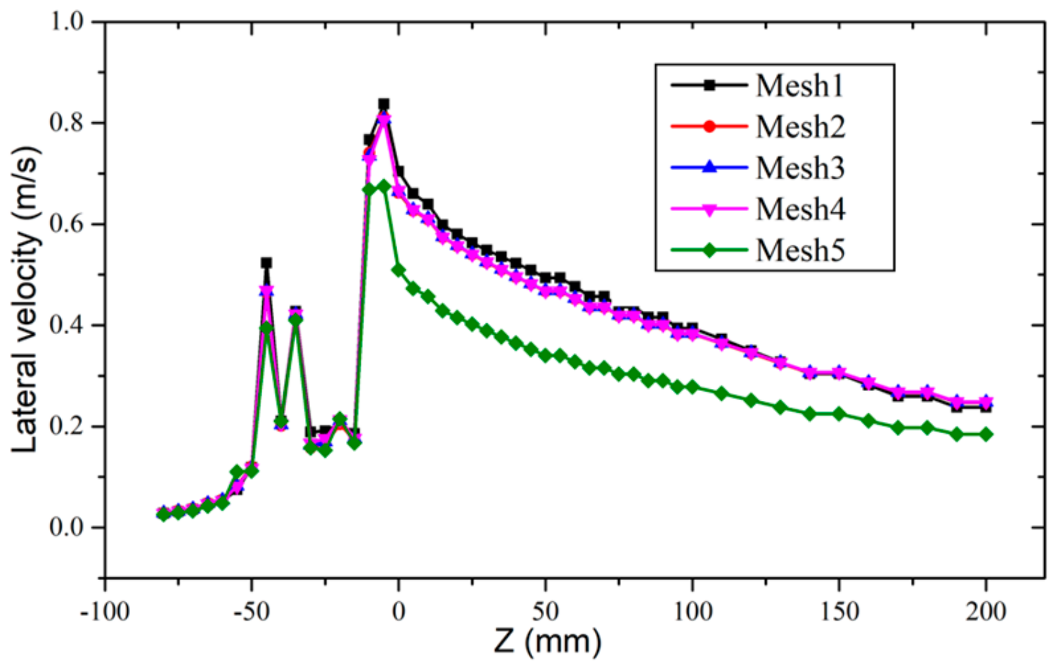
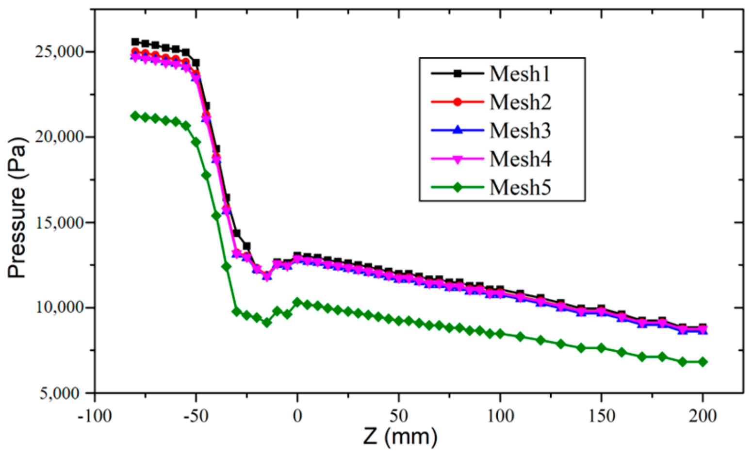
4.1. Mesh Independence Investigation

It is very difficult to verify the mesh independence of the whole fuel assembly model. Because of the very complex geometry, the number of meshes will reach hundreds of millions. Due to the geometric repeatability of the spacer grids, the mesh independence that is established for a single spacer grid will also be established for all the spacer grids. Therefore, the mesh independence study was performed on a single complete spacer grid and its upstream and downstream fuel rod regions were also considered. A 17 × 17 rod bundle model was built in NX UG 9.0 software, which contained a standard AFA-3G spacer grid, 264 fuel rods, and 25 control rods. The spacer grid was composed of strips, mixing vanes, springs, and dimples. In order to make the fluid fully developed in the flow channel, the length of the upstream and downstream rod regions were sufficiently long. According to the geometric structure of the computational domain, the polyhedral mesh and extruded mesh were used to generate the mesh in Star-CCM+ software. The number of mesh and local refinement were controlled by the base size and the minimum size. The minimum cell size and the fluid boundary layer thickness were set as a percentage of this value. The extruded surface was located at 10 mm upstream and 10 mm downstream of the spacer grid. The upstream extruded volume was 400 mm long and the downstream extruded volume was 600 mm long. The extruded mesh is shown in Figure 3a,c and Figure 3b shows the polyhedral mesh.

Five groups of mesh were selected to study the effects of different base sizes and boundary layer heights on the calculation results, as shown in Figure 4. A SST k-ω model was used for the grid independence verification. When the thickness of the first layer was 0.05 mm, 0.075 mm, and 0.1 mm, the average y+ of the rods were 6.6, 10.2, and 13.3, respectively. The size parameters and the number of grids are shown in

Table 1. Mesh parameters.

No.	Base Size (mm)	Min Size at Grid (mm)	First Height of Prism (mm)	Ratio	Prism Layers	Mesh Number
1	2	0.2	0.1	1.2	3	17.17 × 106
2	4	0.4	0.05	1.2	3	8.95 × 106
3	4	0.4	0.075	1.2	3	8.82 × 106
4	4	0.4	0.1	1.2	3	8.69 × 106
5	8	0.8	0.1	1.2	3	3.71 × 106

.

The boundary condition of the mesh independence investigation was consistent with the maximum sub-channel Reynolds number condition of a fuel assembly that had an inlet mass flow of 102 kg/s. The Reynolds number in the sub-channel was 500,000, the temperature of 310 °C was set at the inlet, and the atmospheric pressure was set at the outlet. The water physical property was set to be 15.5 MPa and 310 °C. The upper surface of mixing vanes was taken as the reference plane and z = 0 was set at this surface. The lateral velocity and pressure of the average mass flow in different height surfaces were summarized. The variation of the lateral velocity and pressure along the flow direction were plotted in Figure 5 and Figure 6. Compared with meshes 1, 4, and 5, it was found that all the meshes with a base size of 4 mm were in good agreement with the mesh with a base size of 2 mm. The mesh with a base size of 8 mm had a large deviation from the refined mesh. Compared with meshes 2, 3 and 4, it was found that the thickness of the boundary layer had little effect on the results. Therefore, it was considered that the mesh was independent when the base size was 4 mm and the height of the first boundary layer was 0.1 mm.

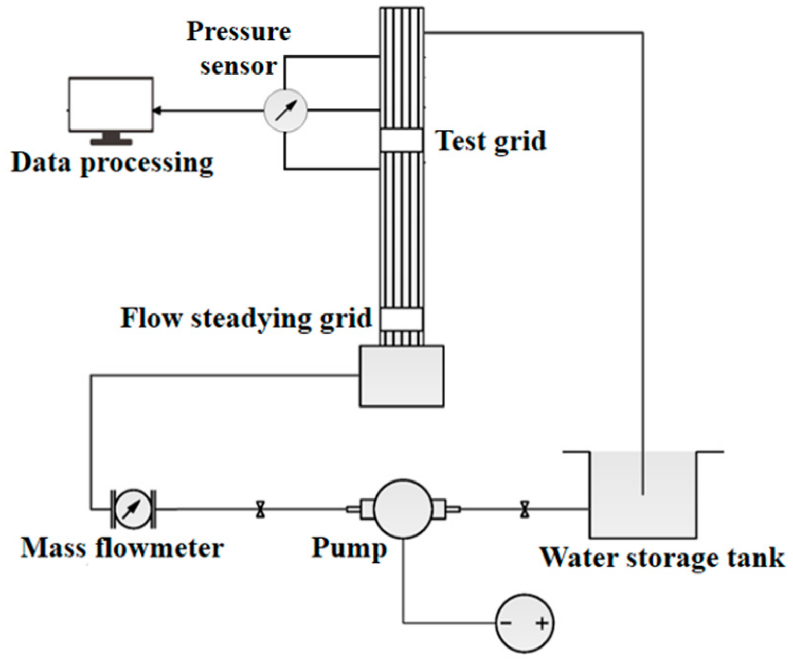
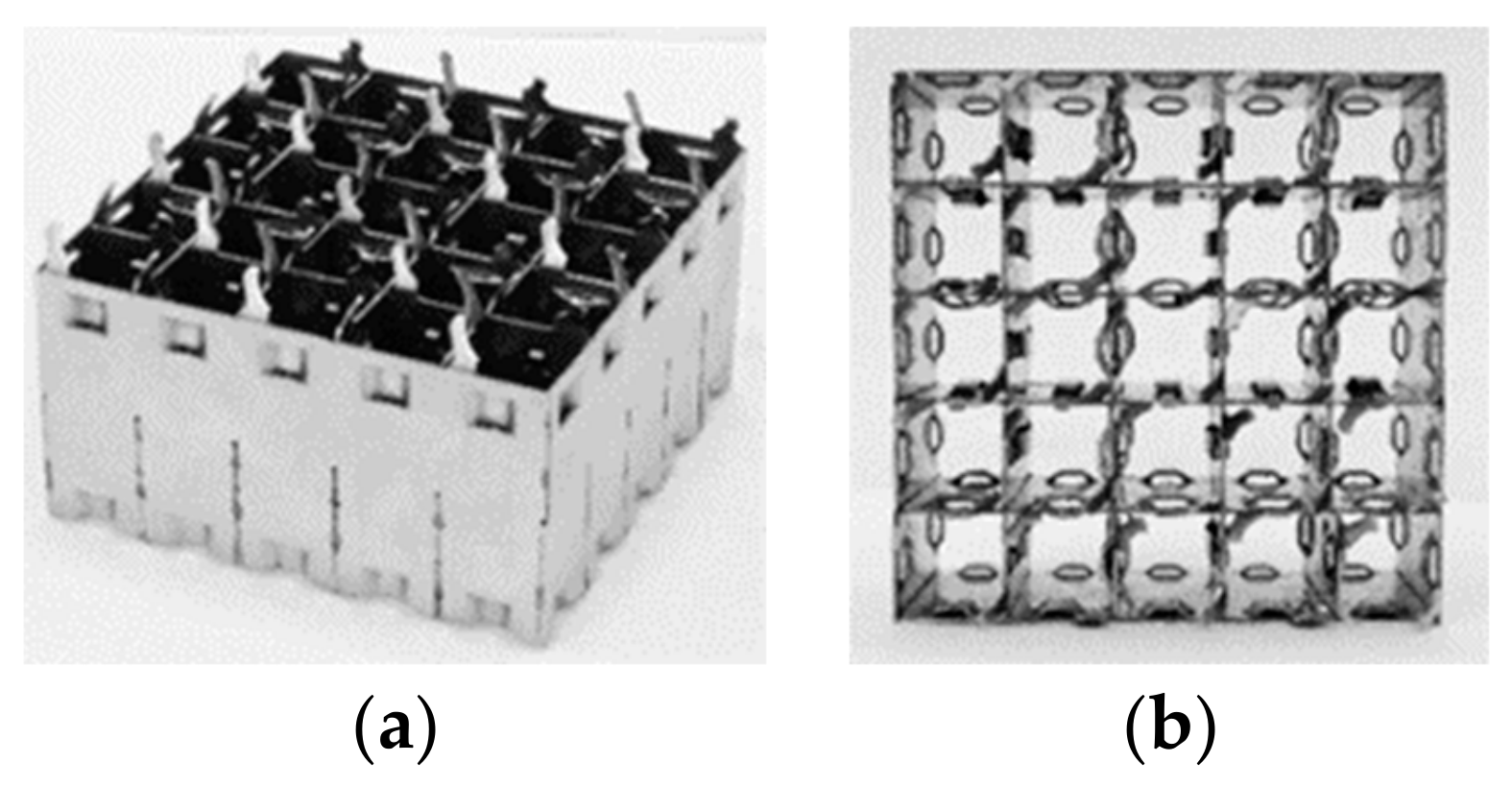
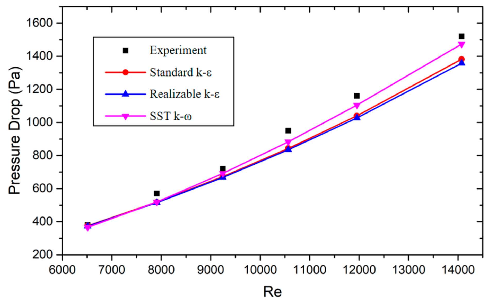
4.2. Turbulence Model Verification

The experimental system consisted of a water storage tank, pipeline centrifugal pump, mass flowmeter, and pressure test section, as shown in Figure 7. The test section consisted of two spacer grids. The first one was the grid of steady flow, which counteracted the flow instability generated by the entrance. The length of the stable flow section was 800 mm. The second one was a 5 × 5 standard AFA-3G spacer grid, which contained springs, dimples, and mixing vanes, as shown in Figure 8. The experiment was carried out at normal temperature and pressure. The deionized water was used as a working fluid and operating conditions were Reynolds numbers 6510 to 14,074 in the sub-channels. After a period of stable operation of the system, the pressure drop data between 10 mm upstream and 10 mm downstream of the spacer grid were measured using a pressure sensor under different working conditions. The average values were repeatedly taken as the reference data and the verification basis for numerical simulations.

A 5 × 5 rod bundle model was built in NX UG software, which contained a standard AFA-3G spacer grid and 25 fuel rods. The spacer grid was composed of strips, mixing vanes, springs, and dimples. The side length of the flow channel was 65 × 65 mm and the diameter of the rod bundle was 9.5 mm. The mesh parameter settings were consistent with the grid independence verification in the previous section. The calculated boundary conditions were consistent with the experiment, as shown in the

Table 2. Boundary conditions.

Position	Parameter	Value
Inlet	Mass flow (t/h)	5.07	6.16	7.20	8.23	9.31	10.96
	Reynolds number	6510	7910	9246	10,568	11,955	14,074
Outlet	Relative pressure (Pa)	0 (Reference-pressure was 101,325 Pa)
Spacer Grid	No slip wall
Wall	No slip wall

.

The flow in the sub-channel of the fuel assembly had a high Reynolds number turbulence and the selection of the turbulence model had a significant influence on the calculation results. This section gives the calculation results of the pressure drop of the spacer grid region under different Reynolds numbers based on the experimental operating conditions, as shown in Figure 9. The results of the SST k-ω model with a low y+ wall treatment mesh and two kinds of k-ε model with a high y+ wall treatment mesh were compared. In addition to the boundary layer, the mesh size parameter settings were completely the same. From the figure, it can be seen that all the calculation results were smaller than the experimental results and the pressure drop obtained by the SST k-ω model was the closest to the experimental results. Combined with previous studies on the applicability of the turbulence model in the flow field of spacer grids, it was also shown that the calculation results of the SST k-ω model were in good agreement with the experimental values [17]. In summary, the SST k-ω model was used for the following calculations.

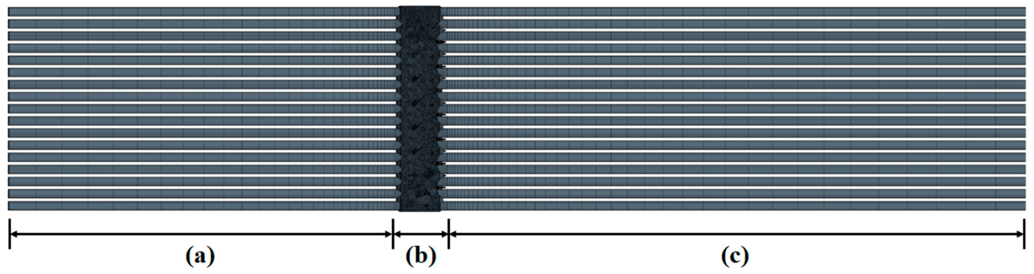
4.3. Mesh Generation for the Whole Fuel Assembly

There is no doubt that the mesh generation of the whole fuel assembly is very difficult. In previous studies, it was even very difficult to generate one 17 × 17 spacer grid with mixing vanes, springs, and dimples, which will occupy a lot of computing resources. In this section, due to the excellent pre-processing and post-processing parallel mechanism of Star-CCM+ software, a complete set of technical methods to generate mesh of the whole fuel assembly has been proposed. The problem that it is difficult to realize the whole fuel assembly CFD simulation has been solved.

The polyhedral mesh was used to capture the flow details of the complex flow field in the grid area, which ensured the accuracy of turbulence calculation. The extruded mesh was used in the fuel rod area without grids because of the regular shape of the sub-channels. Compared with the polyhedral mesh, an extruded mesh will not make the number of meshes particularly large. The flow area between the upstream 10 mm and the downstream 10 mm of the grid was taken for both the mixing grid and the inter-span grid. All components were positioned in the software, as shown in the figure. The polyhedral mesh was used in all areas shown in Figure 10, and the mesh parameter setting was the same as the independence verification mesh. The blank area between each two areas was the fuel rod area without grids and an extruded mesh was used in these areas. Before the generation of the extruded mesh, two surfaces of each of two adjacent areas were set as a periodic repetition to ensure that the mesh nodes on the interface were completely coincident. The base surface of the extruded mesh was the upper surface of each spacer grid region, as shown by the red arrow.

After generating the polyhedral and extruded meshes, there were still interfaces between all regions. In the Star-CCM+ software, adjacent mesh areas can be connected into a continuous and complete area through an interface fusion operation. The fuse command can be used to combine a pair of boundaries from the same volume mesh region and replace them with interior faces. The advantage of removing boundaries by fusing is that there is no additional overhead involved in the calculation (as might be incurred at an interface). Hence, all regions were fused after mesh generation and a set of complete and continuous meshes of the whole fuel assembly was finally obtained, as shown in Figure 11. The mesh quantity is showed in

Table 3. Mesh quantity.

Type	Quantity
Cells	193,023,023
Interior Faces	920,902,717
Vertices	701,831,537

.

4.4. Boundary Conditions and Calculations

The Reynolds number in the sub-channel was 500,000, a temperature of 31 °C was set at the inlet and atmospheric pressure was set at the outlet. The water physical property was temperature-independent and set to 15.5 MPa and 310 °C. The heat flux on the rods’ surfaces was 500 kW/m². A 64-core CPU was used for parallel computation for 72 h. The residual converged to below 10⁻⁴.

5. Results and Discussion

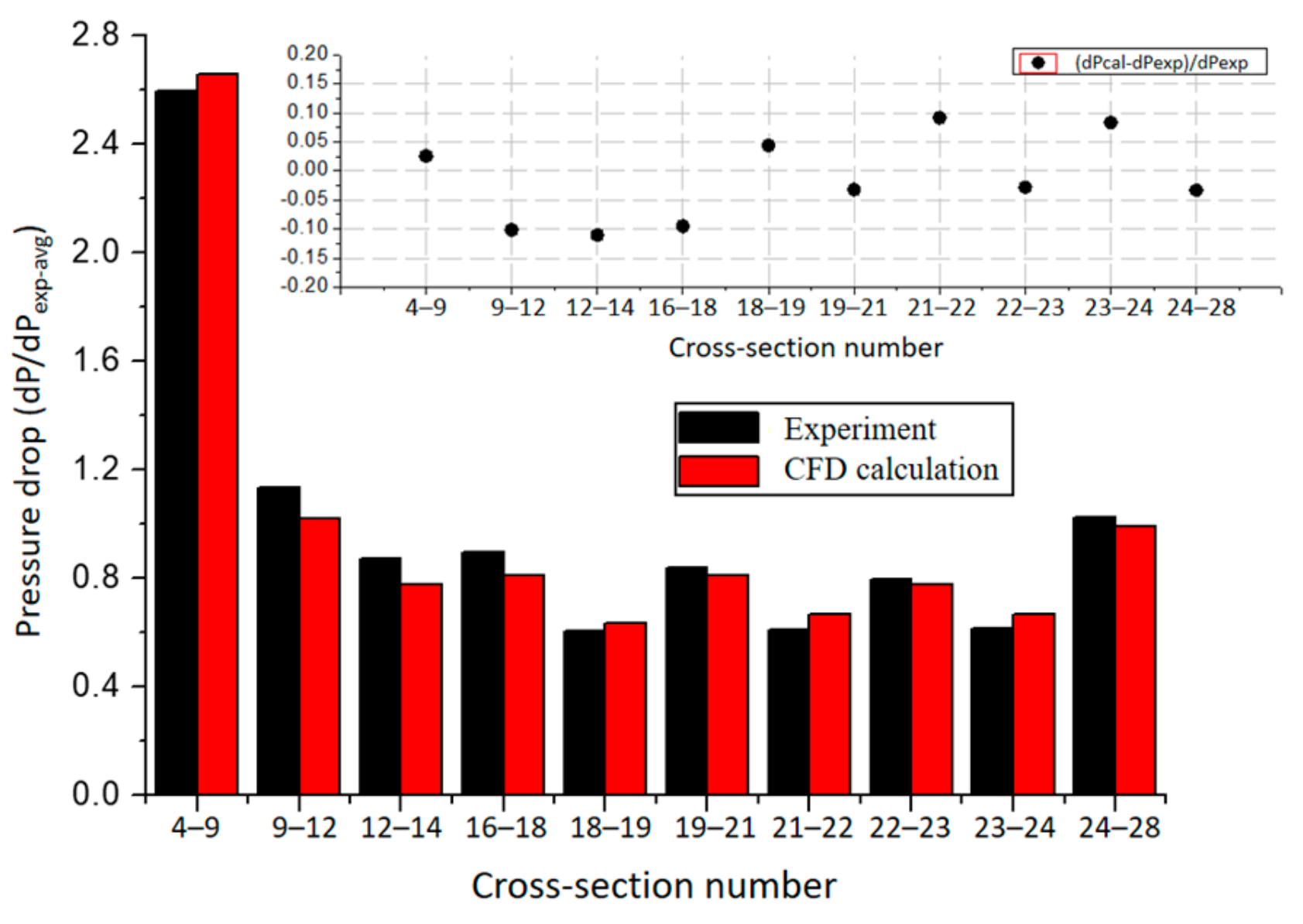
5.1. Pressure Verification

The research condition for the pressure distribution was a 500,000 Reynolds number in the sub-channel, which is the highest Reynolds number condition in the fuel assembly. The velocity in the sub-channel exceeded 6 m/s and the range of the velocity changes also had the maximum range in the reactor operation. According to the momentum equation, the pressure change was also very significant. The significance of the whole fuel assembly numerical simulation was the ability to get the pressure range along the flow direction and to get the pressure drop values of different positions and different types of grids. The integer hydraulic test data of the fuel assembly was used as the benchmark. As shown in Figure 12, the pressure drop between different monitoring planes were obtained. The difference between the calculated and experimental pressure drop was less than 10%, as shown in Figure 13. The calculated pressure drop of the inter-span grids were larger than the experimental results and the calculated pressure drop of the mixing grids were smaller than the experimental results.

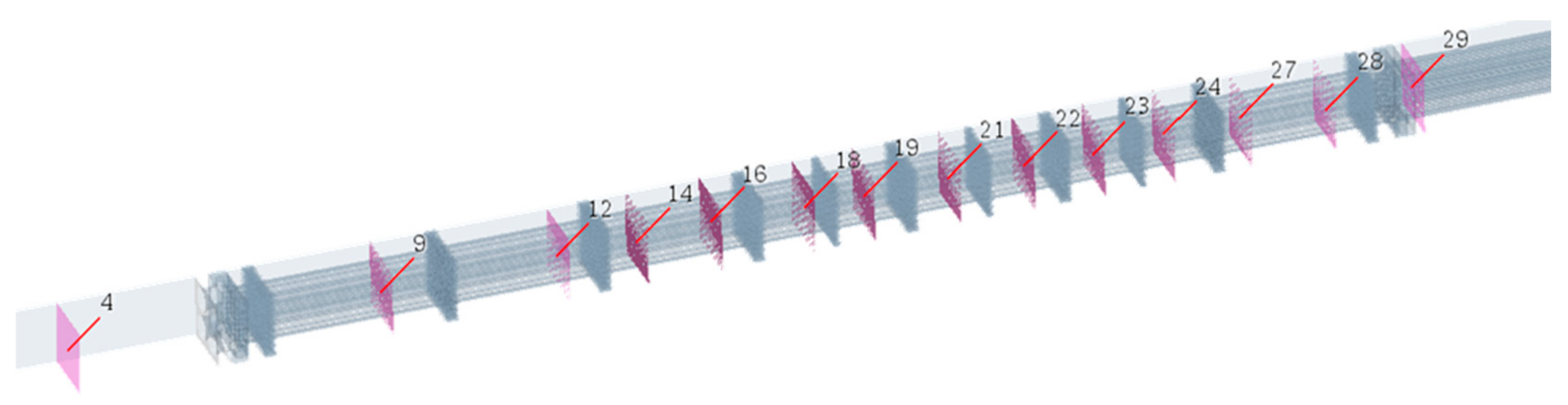
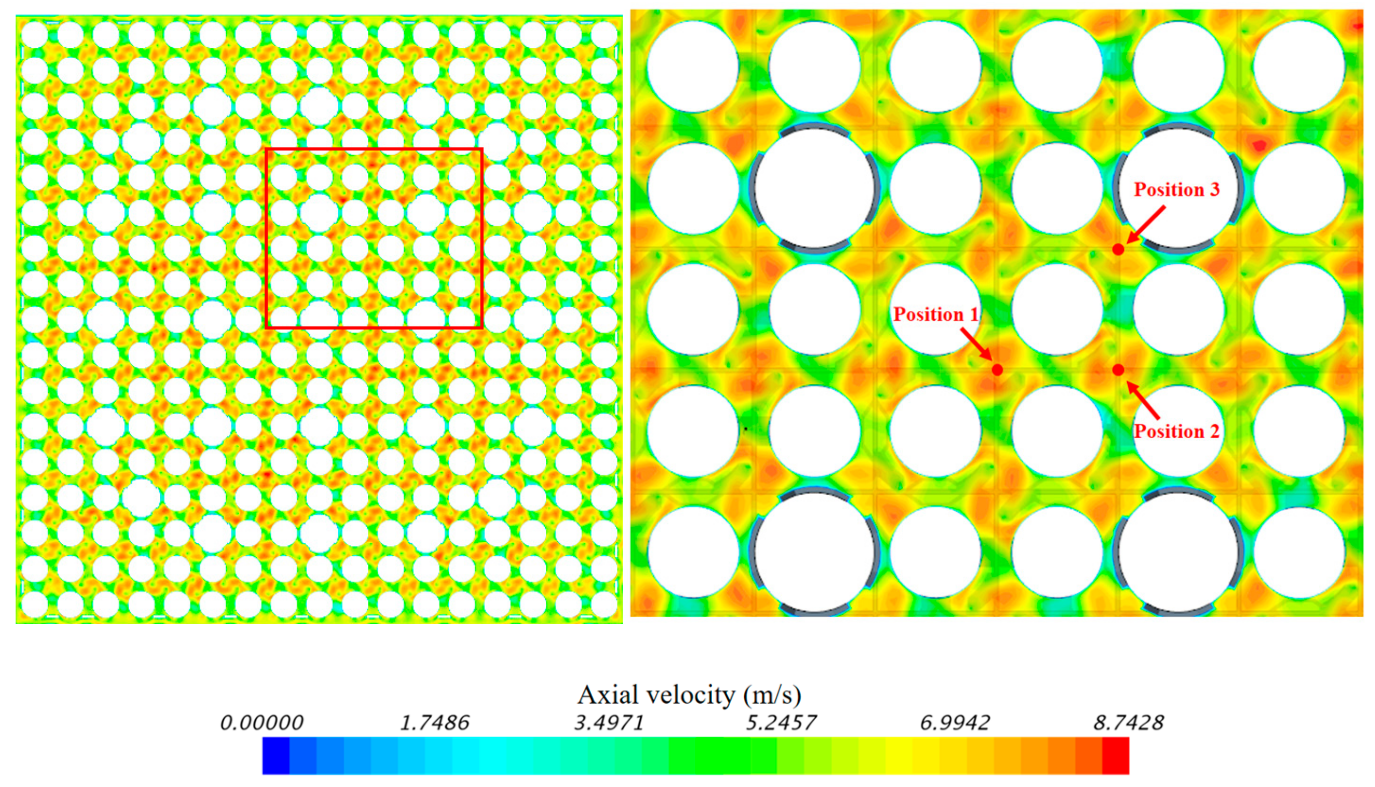
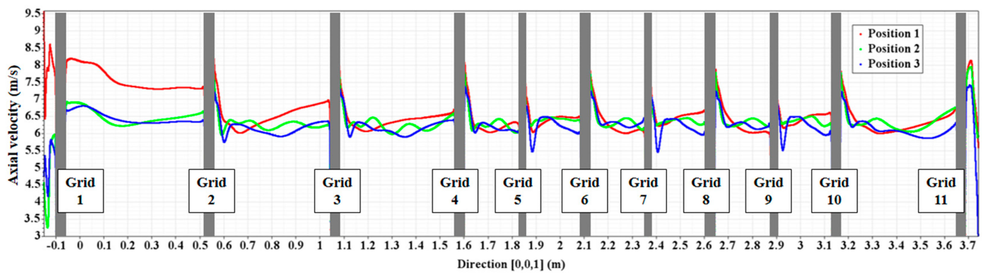
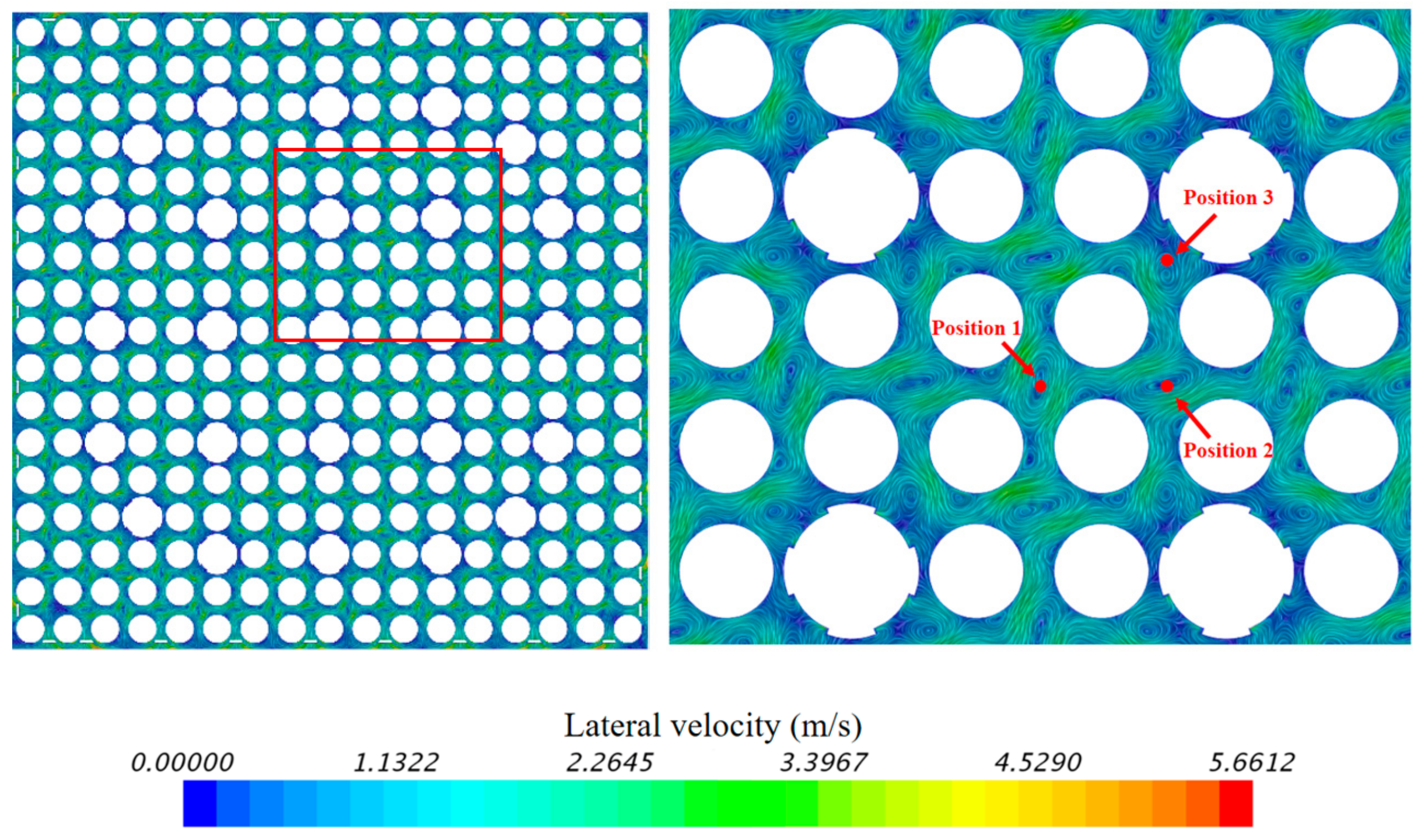
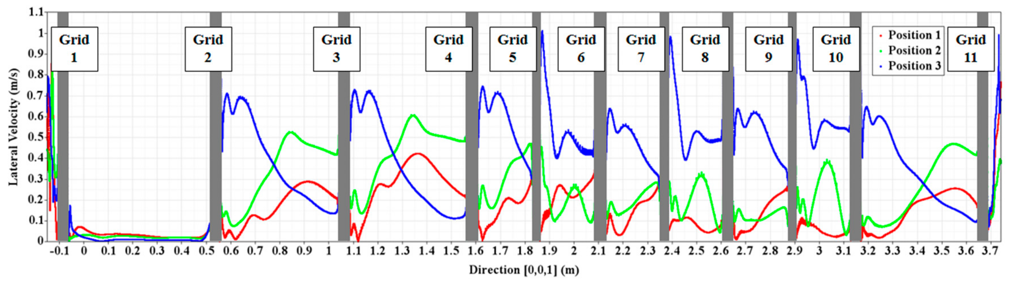
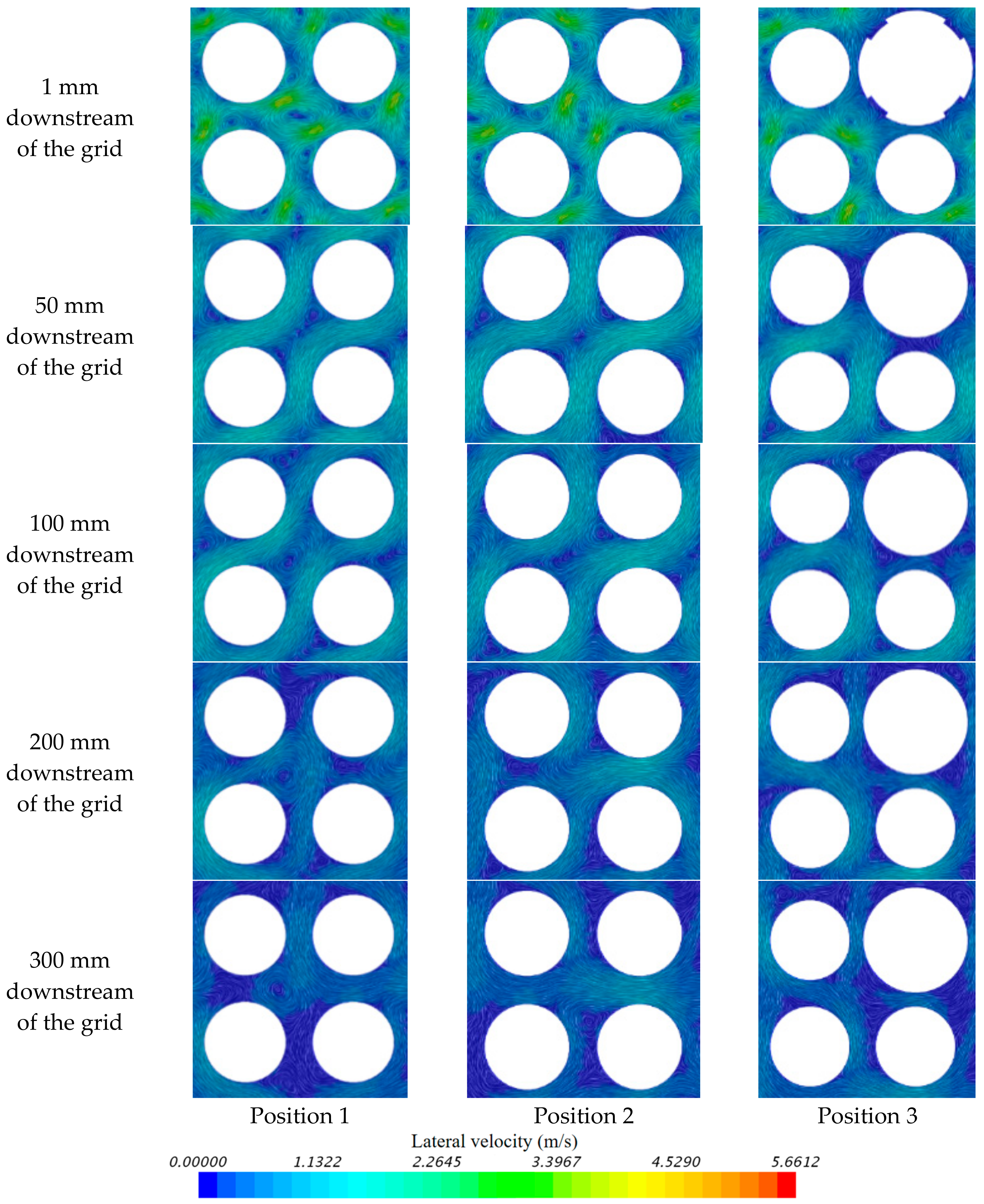
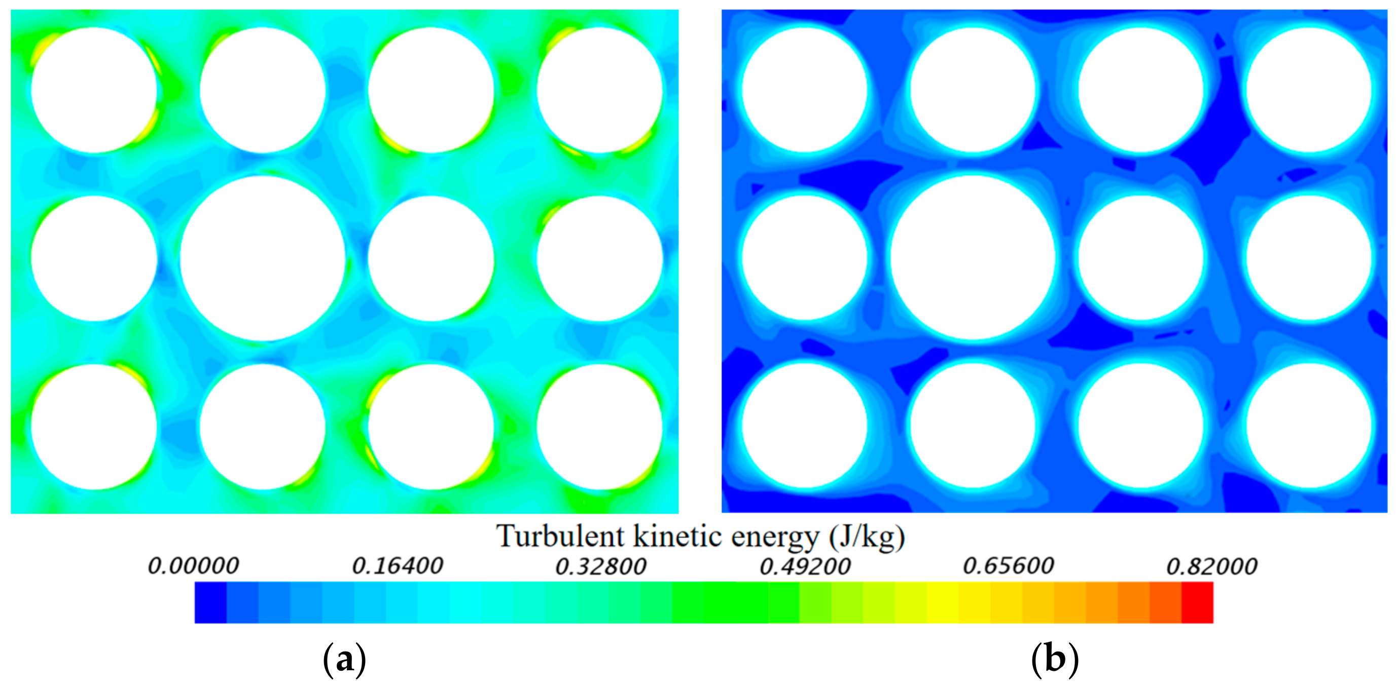
5.2. Velocity Distrubution

The axial velocities at different positions in the sub-channel of the whole assembly were monitored and are shown in Figure 14. The relationship between the axial velocities and the height is shown in Figure 15. When the fluid flowed through the first spacer grid, the axial velocity of position 1 reached 8.25 m/s, which was much higher than that of positions 2 and 3. The velocity decreased slightly after 0.2 m downstream of the grid but the axial velocity of the three sub-channels was still very large. The first grid was the end spacer grid without mixing vanes, which produced a weak lateral flow. Therefore, the flow transfer phenomenon between sub-channels was not obvious and had little effect on the numerical value and distribution of the axial velocity.

After flowing through the second and third grids, the axial velocity of the fluid reached a maximum at the center of the three positions. Then, it decreased rapidly to the lowest at the region of five hydraulic diameters and then increased gradually.

This phenomenon was particularly obvious at the position downstream of the second grid. The axial velocity of position 1 first decreased to 15% lower than that of positions 2 and 3, and then gradually increased to 11% larger than that of positions 2 and 3.

After the fourth, sixth, and eighth grids, which were mixing spacer grids, the change trend of the axial velocity at different locations were basically the same. It decreased rapidly at first, then changed gently, which was consistent with the change downstream of the second and third grids. However, the length of the rod region downstream of these three grids were short, such that the fluid reached the next downstream grid before the axial velocity of position 1 rose significantly. The fifth, seventh, and ninth grids were inter-span grids, which existed to enhance the convective heat transfer in the region with the highest power in the fuel rod bundle. It can be seen that the axial velocities of the fluids in all three positions dropped sharply after passing through these three grids and the axial velocity of position 3 was the lowest, 10% lower than those in positions 1 and 2. After that, the velocity of position 1 remained unchanged or rose slightly, while the velocities of positions 2 and 3 decreased. However, the axial velocity of position 3 decreased earlier than that of position 2. Hence, the axial velocity of position 3 was the lowest among the three positions before reaching the next downstream grid. The downstream axial velocity changing trend of the tenth grid was the same as the second and third grids, but the later velocity growth of position 1 was not obvious.

The lateral velocities at different positions in the sub-channel of the whole assembly were monitored and are shown in Figure 16. The relationship between the lateral velocities and the height is shown in Figure 17.

The lateral velocity downstream of the first grid was weak due to the absence of mixing vanes. The changing trend downstream of the second to tenth grids were similar when the flow was just flowing out of the grids. The lateral velocities of position 3 were much larger than those of position 1 and 2. The maximum lateral velocity of position 3 was twice that of positions 1 and 2, reaching 1 m/s. This was because positions 1 and 2 were located in the center of the sub-channel vortexes and the lateral velocity was much lower than that near the edge of the vortexes and the wall of the fuel rods. The vortex at position 3 was offset by the asymmetry of the sub-channel that was caused by the control rod and the single-mixing-vane structure. Hence, the lateral velocity of position 3 was higher. However, this phenomenon changed downstream for the second, third, and tenth grids, which had longer fluid domains downstream of the grids. After the 0.2–0.3 m area downstream of the grid, the lateral velocity of position 3 was exceeded by positions 1 and 2. At this time, the vortexes at positions 1 and 2 began to migrate and the lateral velocity in the center of the sub-channels increased.

The cross-sectional lateral velocities at different locations downstream of the third grid are shown in Figure 18 and the vortexes at the three locations were obviously different. Because of the long distance from the control rods, the vortexes of position 1 were obviously symmetrical. The maximum velocity was generated near the wall of the two diagonal fuel rods. With the increase of the distance along the flow path, the intensity of the vortexes decreased, forming a figure-eight-shaped flow field with the center located at position 1. The area of larger lateral velocity was generated near the rod wall surface and there was a vortex that was finally formed in the center of the sub-channel.

The form of the vortexes in position 2 was similar to position 1, but the two above and below the adjacent sub-channels were the control rod sub-channels, resulting in the deviation of the vortexes between the two rods in the upper and lower channels. With the increase of the distance along the channel, the vortexes in this position were independent of the figure-eight-shaped flow field and eventually formed a unidirectional flow pattern in the center of the sub-channel. Position 3 was the center of the control rod sub-channel where eccentric vortexes were generated. The lateral velocity was the largest in the three positions, but the intensity of the vortexes decreased rapidly. At 300 mm downstream of the grid, the lateral velocity began to be lower than that at positions 1 and 2. In the process of the development and change of the secondary flow, it could not cover all areas of the rod wall. There was a velocity shadow at local positions near the wall. The flow and heat transfer of these positions were weakened, which was not affected by the secondary flow, resulting in an uneven local temperature distribution, and even produced hot spots.

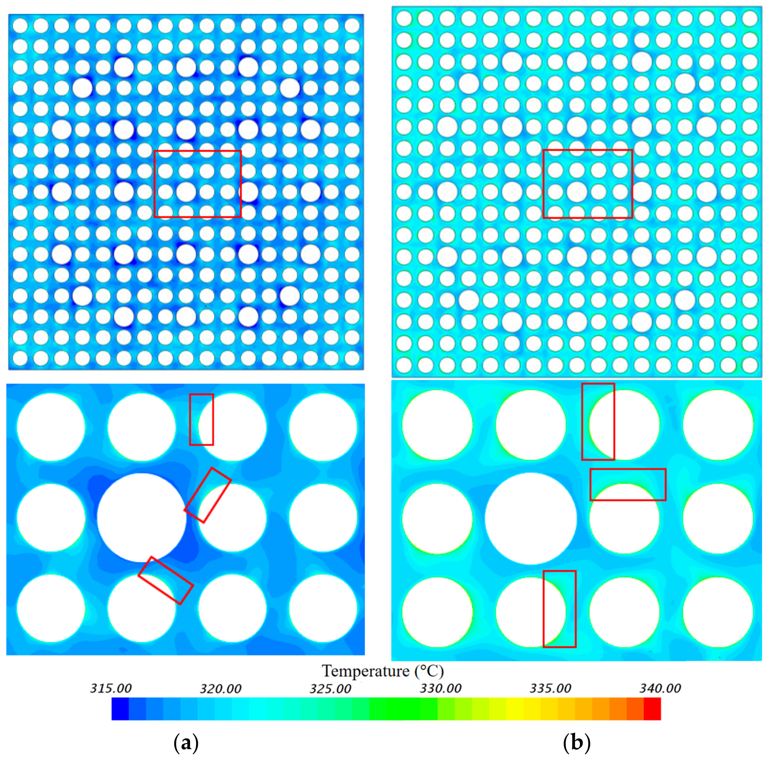
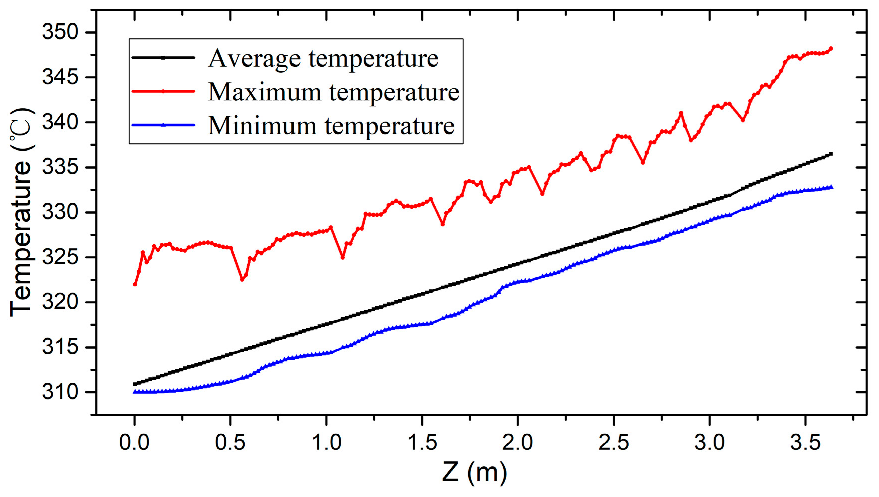
5.3. Temperature Distribution

In this section, the results of the temperature distribution of the fluid is presented. The mass transfer between the sub-channels decreased with the decrease of the lateral flow downstream of the spacer grid. Therefore, the lateral velocity intensity on the rod surface was weakened. The fluid temperature near the rod surface rose. Because there was no heating on the control rod, the temperature distribution in the downstream area near the control rod was very uneven. The temperature field on the plane that was 5 mm and 400 mm downstream of the third mixing grid are shown in the Figure 19. It can be seen that the temperature distribution at different distances downstream were different. In particular, the temperature of the fluid near the rod surface was very high at position z = 400 mm downstream of the spacer grid.

It can be seen from the velocity field of the last section that the mass transfer between adjacent sub-channels was significant when the fluid was just out of the grid. The flow velocity on the fuel rod wall reached the extreme values and the turbulent kinetic energy near the wall clearly increased, as shown in Figure 20. At this time, the heat transfer between the fuel rod wall and flow was significantly enhanced and the fluid took more heat away. Therefore, the temperature growth of the fluid near the fuel rod wall was not significant; only a small increase existed in the velocity shadow of the secondary flow mentioned in the last section.

At 400 mm downstream of the grid, the lateral velocity decayed to a very low level and the turbulent kinetic energy near the wall was greatly reduced. The heat taken away by the fluid was reduced such that the local fluid near the wall was rapidly heated to a high temperature.

The changes of the average temperature, maximum temperature, and minimum temperature in different height sections are shown in Figure 21. It can be seen that the effect of the spacer grids on the maximum temperature was very significant. In particular, for the area that was just outside of the grid, the maximum temperature downstream of the mixing grid suddenly dropped by 3–4 °C and the maximum temperature downstream of the inter-span grid suddenly dropped by 1–2 °C. The minimum temperature rose steadily and was always distributed near the control rod.

6. Conclusions

In this study, a numerical study of the turbulence flow in a full-scale 17 × 17 fuel assembly was carried out. The main conclusions are summarized as follows:

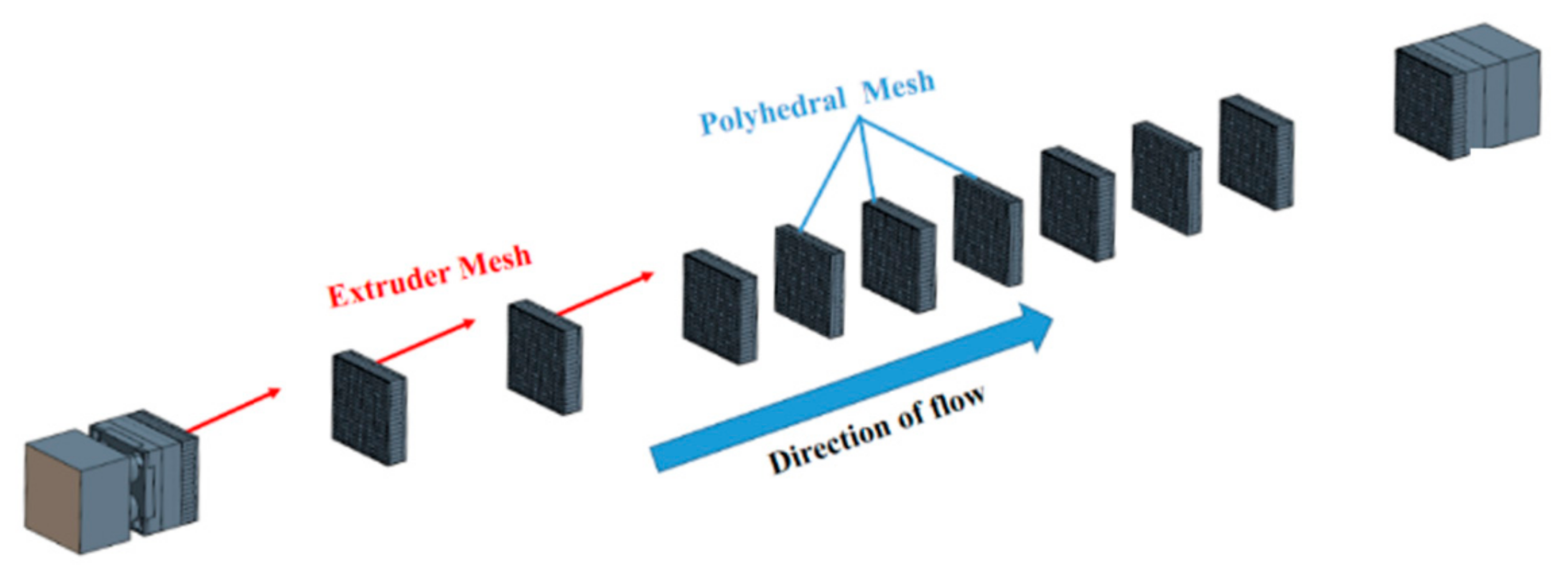
• In the Star-CCM+ software, the full-scale fuel assembly could be simulated and analyzed using using polyhedral and extruded meshes. The total number of meshes for the complete fuel assembly was 193 million. The mesh model was verified using independent verification and the SST turbulence model was verified by small-scale experiments.
• The results of the pressure drop in the whole fuel assembly was verified by the integer hydraulic test data of the fuel assembly. The calculation and experiment pressure drop difference was less than 10%.
• The difference in the axial velocity between the different sub-channels occurred only when the rod region downstream of the grid was longer. On the contrary, the lateral velocity in the control rod sub-channel was clearly higher than that in other channels, which was caused by the generation and migration of different vortexes in the sub-channels.
• There was a velocity shadow at local positions near the wall, resulting in an uneven local temperature distribution, and even produced hot spots. The presence of the spacer grid had a significant effect on the maximum temperature of the fluid near the fuel rod wall, but had little effect on the minimum temperature.

References

1. McClusky, H.L.; Holloway, M.V.; Conover, T.A.; Beasley, D.E.; Conner, M.E.; Smith, L.D. Mapping of the lateral flow field in typical sub-channels of a support grid with vanes. J. Fluids Eng. 2003, 125, 987. [Google Scholar] [CrossRef]
2. Holloway, M.V.; McClusky, H.L.; Beasley, D.E.; Conner, M.E. The effect of support grid features on local, single-phase heat transfer measurements in rod bundles. J. Heat Transf. 2004, 126, 43. [Google Scholar] [CrossRef]
3. Holloway, M.V.; Conover, T.A.; McClusky, H.L.; Beasley, D.E.; Conner, M.E. The effect of support grid design on azimuthal variation in heat transfer coefficient for rod bundles. J. Heat Transf. 2005, 127, 598. [Google Scholar] [CrossRef]
4. Conner, M.E.; Baglietto, E.; Elmahdi, A.M. CFD methodology and validation for single-phase flow in PWR fuel assemblies. Nucl. Eng. Des. 2010, 240, 2088–2095. [Google Scholar] [CrossRef] [Green Version]
5. Karoutas, Z.; Gu, C.Y. 3-D flow analyses for design of nuclear fuel spacer. In Proceedings of the Seventh International Meeting on Nuclear Reactor Thermal-Hydraulics, New York, NY, USA, 10–15 September 1995. [Google Scholar]
6. Seok, K.C.; Sang, K.M.; Won, P.B.; Young, D.C. Phenomenological investigations on the turbulent flow structures in a rod bundle array with mixing devices. Nucl. Eng. Des. 2008, 238, 600–609. [Google Scholar]
7. Sang, Y.H.; Jeong, S.S.; Min, S.P.; Young, D.C. Measurements of the flow characteristics of the lateral flow in the 6 × 6 rod bundles with Tandem Arrangement Vanes. Nucl. Eng. Des. 2009, 239, 2728–2736. [Google Scholar]
8. Conner, M.E.; Hassan, Y.A.; Dominguez-Ontiveros, E.E. Hydraulic benchmark data for PWR mixing vane grid. Nucl. Eng. Des. 2013, 264, 97–102. [Google Scholar] [CrossRef]
9. Wang, K.I.; Dong, S.O.; Tae, H.C. Flow Analysis for Optimum Design of Mixing Vane in a PWR Fuel Assembly. J. Korean Nucl. Soc. 2001, 33, 327–338. [Google Scholar]
10. Cui, X.Z.; Kim, K.Y. Three Dimensional Analysis of Turbulent Heat Transfer and Flow through Mixing Vane in A sub-channel of Nuclear Reactor. J. Nucl. Sci. Technol. 2003, 40, 719–724. [Google Scholar] [CrossRef]
11. Holloway, M.V.; Beasley, D.E.; Conner, M.E. Investigation of swirling flow in rod bundle sub-channels using computation fluid dynamics. In Proceedings of the ICONE 14 International Conference on Nuclear Engineering, Miami, FL, USA, 17–20 July 2006. [Google Scholar]
12. Nematollahi, M.R.; Nazifi, M. Enhancement of heat transfer in a typical pressurized water reactor by different mixing vanes on spacer grids. Energy Convers. Manag. 2008, 49, 1981–1988. [Google Scholar] [CrossRef]
13. Yan, B.H.; Gu, H.Y.; Yang, Y.H.; Yu, L. Effect of rolling on the flowing and heat transfer characteristic of turbulent flow in sub-channels. Prog. Nucl. Energy 2011, 53, 59–65. [Google Scholar] [CrossRef]
14. Liu, C.C.; Ferng, Y.M.; Shih, C.K. CFD evaluation of turbulence models for flow simulation of the fuel rod bundle with a spacer assembly. Appl. Therm. Eng. 2012, 40, 389–396. [Google Scholar] [CrossRef]
15. Ikeno, T.; Kajishima, T. Analysis of dynamical flow structure in a square arrayed rod bundle. Nucl. Eng. Des. 2010, 240, 305–312. [Google Scholar] [CrossRef]
16. Bae, J.H.; Park, J.H. Analytical prediction of turbulent friction factor for a rod bundle. Ann. Nucl. Energy 2011, 38, 348–357. [Google Scholar] [CrossRef]
17. Li, Q.; Chen, J.; Jiao, Y.H. Research on Resistance Features of a 5 × 5 Rod Bundle with Spacer Grid. Nucl. Power Eng. 2015, 36, 28–32. [Google Scholar]
Figure 1. Geometric model of a full-scale fuel assembly: (a) the fuel assembly with fuel rods, (b) the fuel assembly without fuel rods, (c) the main view of the spacer grid, and (d) the top view of the spacer grid.
Energies 13 00397 g001aEnergies 13 00397 g001b
Figure 2. Geometric model of a mixing grid.
Energies 13 00397 g002
Figure 3. Different kinds of mesh: (a) extruded mesh; (b) polyhedral mesh; (c) extruded mesh.
Energies 13 00397 g003
Figure 4. Meshes used for independence verification. (a) Mesh1, (b) Mesh2, (c) Mesh3, (d) Mesh4, (e) Mesh5.
Energies 13 00397 g004
Figure 5. Distribution of the lateral velocity for different meshes.
Energies 13 00397 g005
Figure 6. Distribution of the pressure for different meshes.
Energies 13 00397 g006
Figure 7. Experimental system.
Energies 13 00397 g007
Figure 8. A 5 × 5 standard AFA-3G spacer grid: (a) the main view of the spacer grid and (b) the top view of the spacer grid.
Energies 13 00397 g008
Figure 9. Pressure drop by different turbulence models.
Energies 13 00397 g009
Figure 10. Mesh generation of the full-scale model.
Energies 13 00397 g010
Figure 11. Mesh of the whole fuel assembly.
Energies 13 00397 g011
Figure 12. Pressure drop monitoring planes.
Energies 13 00397 g012
Figure 13. Pressure drop compared to experiment.
Energies 13 00397 g013
Figure 14. Location of the monitoring points.
Energies 13 00397 g014
Figure 15. Change of the axial velocity along the flow direction.
Energies 13 00397 g015
Figure 16. Location of the monitoring points.
Energies 13 00397 g016
Figure 17. Change of the lateral velocity along the flow direction.
Energies 13 00397 g017
Figure 18. Cross-sectional lateral velocities at different locations.
Energies 13 00397 g018
Figure 19. Temperature field in the plane downstream of the third mixing grid: (a) 5 mm downstream of the grid and (b) 400 mm downstream of the grid.
Energies 13 00397 g019
Figure 20. Turbulent kinetic energy in the plane downstream of the third mixing grid: (a) 5 mm downstream of the grid and (b) 400 mm downstream of the grid.
Energies 13 00397 g020
Figure 21. Changes in temperature with height.
Energies 13 00397 g021