Article

Thermofluid Modelling of Large-Scale Orchards for Optimal Design and Control of Active Frost Prevention Systems

1
Department of Electrical and Electronics Engineering, Imperial College London, London SW7 2AZ, UK
2
Department of Rural and Biosystems Engineering, Chonnam National University, Gwangju 61186, Korea
3
Dipartimento di Ingegneria Industriale e Scienze Matematiche, Università Politecnica delle Marche, DIISM, via Brecce Bianche 1, 60131 Ancona, Italy
*
Author to whom correspondence should be addressed.
Energies 2020, 13(2), 378; https://doi.org/10.3390/en13020378
Submission received: 9 December 2019 / Revised: 9 January 2020 / Accepted: 9 January 2020 / Published: 13 January 2020
(This article belongs to the Section B: Energy and Environment)

Abstract

:
Accurate modelling and simulation of temperature dynamics in large-scale orchards is important in many aspects, including: (i) for the calculation of minimum energy required to be used in optimal design of active frost prevention energy systems (fully renewable or partially renewable) to prevent freezing of fruit flowers, buds, or leaves; (ii) for testing frost prevention control systems before real-implementation which regulate active heating systems inside orchards targeted to prevent frost. To that end, in this study, first, a novel and sophisticated parametric computational thermofluid dynamics (CTFD) model for orchard air thermal dynamics for different orchard parameters (such as fruit type, climate, number of trees, their sizes, and distance between them) and boundary/initial conditions was developed and validated with field data from the literature. Next, the use of the developed parametric CTFD model was demonstrated through a case study to calculate the minimal thermal energy required to prevent frost under different frost levels in a test Prunus armeniaca orchard located in Malatya, Turkey, which is the world capital for dry apricot production.

1. Introduction

High quality and diversity horticulture outputs (fruits) contribute to national health and wealth through providing a rich nutrition content and export incomes (for example, ≈€15–20 billion for EU member states [1]). However, the horticultural activity and diversity level in each country is different, depending on climate and land properties. For many fruit types which are vulnerable to low temperature levels, frost occurrence is a serious issue affecting both quantity and quality of yield. Although withering of fruit buds/flowers due to frost is dependent not only on temperature levels below 0 C, but also on humidity, wind, whether the period is budding, flowering or early fruit period, and varieties of fruit trees, temperature levels below 0 C have the potential to cause frost events, and hence are the main parameters to control for prevention of yield loss due to frost [2,3].
Active frost prevention methods (such as use of wind machines and heaters [4]) are widely used methods with better frost protection capabilities compared to passive ones (such as site selection, selection of species, and soil management [5]). For any active frost prevention method, it is vital to predict the orchard air and/or canopy temperature to determine the minimum energy requirement to prevent the frost, and to optimally design and control the associated energy providing system in order to minimize the investment and operational costs. Accurate prediction of orchard air and/or canopy temperature in large-scale orchards, in turn, requires modelling thermofluid dynamics of the canopy and the air surrounding trees, which is a daunting task.
In this paper, our contributions are as follows. We develop a detailed parametric computational thermofluid dynamics (CTFD) model to simulate the orchard air and canopy temperatures and airflow in large-scale orchards under different parameters (such as fruit type, climate, the number of trees, their sizes, and distances between trees) and initial/boundary conditions. The developed model is simulated under different frost levels and the temperature prediction results are compared with field measurements under similar conditions from the literature. Next, the use of the developed model is demonstrated through calculation of minimal thermal energy required to prevent frost in a test Prunus armeniaca orchard. Finally, the potential uses of the developed model for optimal design and control of renewable energy-based active frost prevention systems are briefly discussed, and an example framework is given.
In the literature, the problem considered in this paper has been rarely reported. However, there exist some streams of studies on closely related problems. For example, some numerical studies have been done to simulate the potential risk of the frost in order to investigate the influence of the related factors. In an early study, Avissar and Mahrer [6] developed a three dimensional model to simulate the local scale microclimate near the ground during radiative frost events at night considering topography, vegetation, soil humidity, wind speed and direction, and air humidity of the site. In Robinson and Mort [7], for the prediction of frost occurrence, an artificial neural network model was developed and tested in an Italian citrus orchard. The developed system produced two false alarms and one failure of prediction over 50 days, showing that the prediction system still needs some degree of human judgment. In Prabha and Hoogenboom [8], a meso-scale weather forecast was used for the frost prediction. Rahimi and Eccel [9] developed a multiple regression model that predicts the frost occurrence and expected damages on apple trees from meteorological and geographical characteristics of the sites, such as minimum temperature, terrain slope, and frost duration.
Another closely related stream of works evaluated the performance of frost prevention measures numerically. In Issa [10], a simplified heat transfer model was developed to simulate the frost protection of a single citrus fruit using a water spray system. The simulation investigated the effect of air temperature, air speed, and spraying frequency on the solidification of ice layers on the fruit. The recent study by Wenye et al. [11] used a computational fluid dynamics simulation model to develop a wind machine impeller for frost protection, but the simulation model was used to investigate the impeller’s aerodynamic performance rather than to evaluate its performance of frost protection. Although this numerical study can complement troublesome tasks of experimental works, it has limited ability to mimic the temporal variation of complicated microclimate during potential frost events.
The third stream of works (and the most related) in the literature considered air flow around and through trees [12,13,14]. For example, Hong et al. [14] investigated airflow inside tree canopies discharged from air-assisted sprayers through a sophisticated CFD modelling.
The following sections detail the CTFD model development for air dynamics in large-scale fruit orchards, an example demonstrating its use, and a brief discussion for its other potential uses. The nomenclature for the acronyms and symbols used in the paper is provided at the end of the paper.

2. Parametric Computational Thermofluid Dynamics Model Development

2.1. Orchard Parameters and Computational Domain

A generic rectangular prism type fruit orchard with dimensions L m × W m × H m (H is the height of trees) and consisting of n subzones is considered. We assume one hot air blower per zone to heat air around the trees in each zone for frost prevention during frost periods. The distance between roots of trees is s m. The 2-D geometry of the described generic orchard is given in Figure 1. We assume the diameter (the diameter of the approximately circular region covered by branches of a tree) to be d m. The climate data (consisting of wind speed, wind direction, and sky and ground temperatures) are also taken as model inputs.
A computational domain with a size of 2 L m × 2 W m × 5 H m was designed by giving minimum L / 2 m and W / 2 m for buffer zones on longitudinal and transverse edges of the orchard, respectively. Additionally, these buffer zones should be greater than 10 H , which is the minimum relative distance required between the objects and nearby boundaries, according to Bjerg et al. [15], to ensure computational stability against the propagation of pressure between the objects and nearby boundaries. The height of the computational domain should be at least 5 H (suggested by Bjerg et al. [15]); again, for computational stability. The computational domain consisted of millions of structured hexaedron cells. Horizontal dimensions of cells were 1 m within the orchard zones, while they increased gradually in the buffer zones with a geometric ratio of 1.04. At cells adjacent to the ground, the cell height was designed to be 0.01 m and increased gradually upward. The fruit trees were modelled by porous media with a curved cone shape, which is a reasonable approximation for the shape of most fruit trees. The trees were modelled in the computational domain by setting appropriate source terms for momentum loss and turbulence generation to grid cells. These source terms were calculated only for the grid cells located within the trees. This modelling method and the details of the source terms for momentum loss and turbulence generation due to tree canopies are described well by Hong et al. [14,16]. The CFD simulations were performed using ANSYS Fluent CFD code (version 18.2, Ansys, Inc., Canonsburg, PA, USA).

2.2. CFD for Canopy Air Flows

Air flows within and around the orchard were solved by conservation equations for mass, momentum, and energy. For the mass and momentum equations, this study uses the Reynolds-averaged Navier–Stokes (RANS) equations, which is a CFD approach to decompose the Navier–Stokes equations into the mean and fluctuating components. The RANS equations are given as:
ρ t + ( ρ u i ) x i = 0
( ρ u i ) t + ( ρ u i u j ) x j = p x i + x j μ u i x j + u j x i ρ u i u j ¯ + S u i ,
where ρ is the density of air, u is the mean air velocity, u is the fluctuating part of air velocity, p is the air pressure, μ is the air viscosity, and S u i is the source term for the momentum loss due to tree canopies.
The Reynolds stresses, ρ u i u j ¯ , were modelled by the mean velocity gradients using the Boussinesq hypothesis [17] in order to close the RANS equations:
ρ u i u j ¯ = μ t u i x j + u j x i 2 3 ρ k + μ t u k x k δ i j ,
where μ t is called the turbulent air viscosity and it was computed as a function of k (turbulent kinetic energy) and w (specific dissipation rate), which were modelled by the k w turbulence transport model [18].
The source term for the momentum loss due to tree canopies was modelled by the pressure loss coefficient, C i r , as:
S u i = C i r 1 2 ρ | u i | u i , if c g C g , t r e e 0 , if c g C g , t r e e .
Here the pressure loss coefficient C i r is inversely proportional to the density of the tree canopy; c g is the specific grid cell for which the source term is calculated; and C g , t r e e is the group of grid cells located within trees [14].
Transport of energy in the canopy flow is calculated by:
t ρ E + · u ρ E + p = · k e f f T h J + S h
where E is the total air energy (sum of internal and kinetic energy) and calculated as E = h p ρ + u 2 2 with h denoting the sensible air enthalpy (absolute enthalpy minus enthalpy of formation); k e f f is the effective air conductivity, which is the sum of thermal conductivity and turbulent thermal conductivity; T is the air temperature; J is the diffusion flux of any species which arises due to gradients of concentration and temperature; and S h is the air source term which can be decomposed into the sum two sub-terms:
S h = S s e + S s h ,
where S s e is the sensible heat exchange term between the plant and the air ( W / m 3 ); and S s h is the sensible heat generation from space heaters located in each zone ( W / m 3 ). The hot air blowers were not modelled geometrically in the CFD model, but their sensible heat addition to the air was considered as S s h term in Equation (6).

2.3. CFD-Based Thermophysics Analysis of Frost in Fruit Orchards

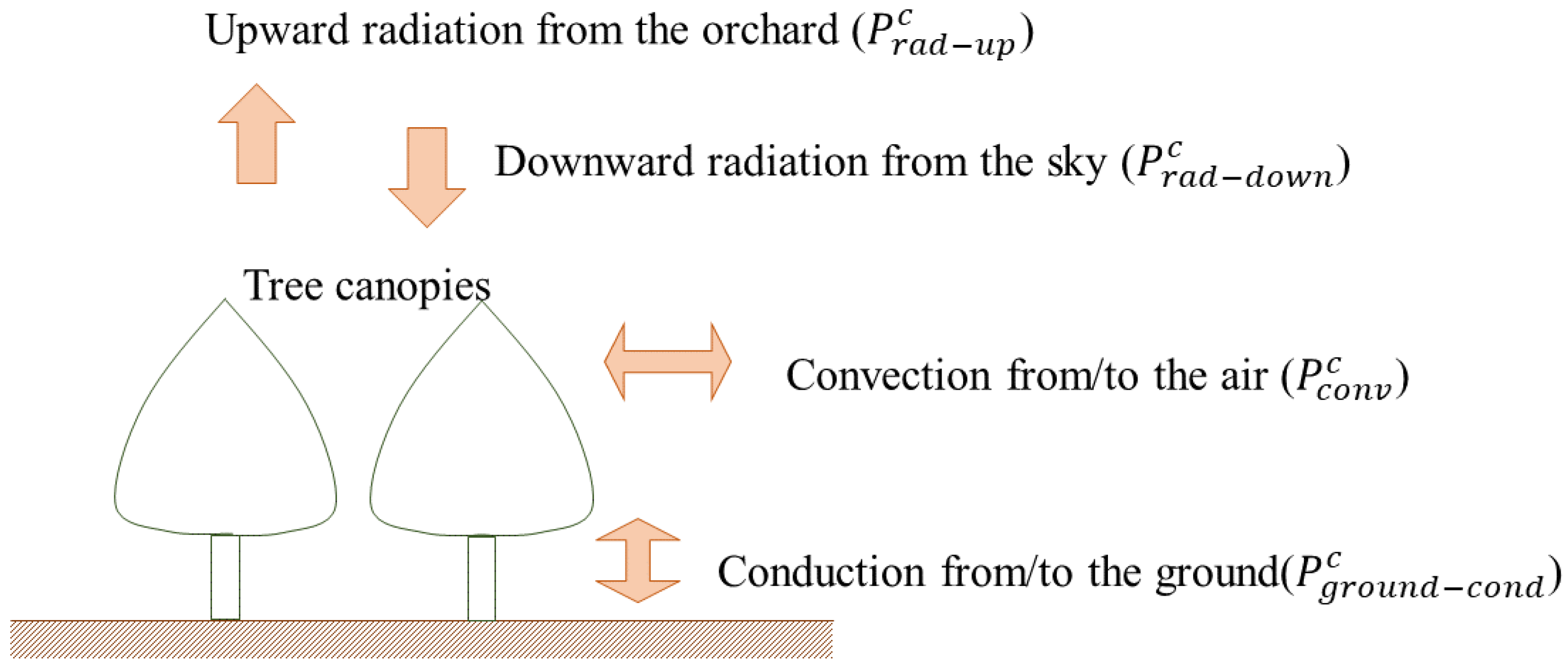
As shown in Figure 2, the thermophysics of fruit orchards involves complicated energy fluxes between trees and their surroundings. During the night time, trees in the orchard lose energy through radiation upward, and at the same time gain the energy downward from the sky. During frost periods, the trees lose more energy than they gain from the sky because at these times the sky temperature is always lower than the temperature of the tree or the ground. Under a clear sky, more heat is lost than gained, while cloudy or foggy skies decrease the energy loss because the temperature of the clouds is higher than the sky temperature. Besides the radiation transfer, trees also exchange their energy with the ground through conductive heat transfer, and with the surrounding air through convective heat transfer. The combined heat transfer to and from the trees determines the variation of their canopy temperature.
Physical parameters associated with the canopy of a fruit orchard are described in Table 1. While these parameters vary by individual trees and their growth conditions, this study assumed that all trees were identical with respect to the shape and canopy condition, which are, in general, reasonable assumptions for typical trees in an orchard.
Next, the expressions for each of the energy transfers in Figure 2 using the canopy parameters in Table 1 are given. The outgoing radiation from the tree canopy can be calculated using the Stefan–Boltzmann law as:
P rad - up c = 1 L A I ϵ σ T c 4 ,
where P rad - up c is the radiation heat flux from the tree canopy to the sky per leaf area ( W / m 2 ); L A I is the leaf area index of the tree ( m 2 / m 2 ); ϵ is the emissivity and approximately 0.74 for the night sky; σ is the Stefan–Boltzmann constant, 5.67 × 10 8 W / ( m 2 K 4 ) ; and T c is the temperature of the tree canopy (K).
Similarly, the downward radiation flux from the sky to the tree canopy can be calculated by applying the sky temperature to the Stefan–Boltzmann law. However, atmospheric and cloud conditions disturb the exact calculation of the downward radiation. In addition, water vapour in the atmosphere absorbs the radiation and creates another source of radiation. This complexity has been solved through empirical formulas, one of which is the downward radiation model of Goforth et al. [19], a modified version of the Swinbank model [20]:
P rad - down c = 8.78 × 10 12 L A I 1 + K C 2 T 5.852 R H 0.07195 ,
where P rad - down c is the radiation heat flux from the sky to the tree canopy per leaf area ( W / m 2 ); K is a constant, 0.34 for cloud height ≤ 2 km, 0.18 for 2 km < cloud height < 5 km, and 0.06 for cloud height ≥ 5 km; C is the cloud cover constant varying 0.0 for clear sky through 1.0 for totally overcast; T is the air temperature (K); and R H is the relative humidity (%).
The convective heat exchange between the tree canopy and the surrounding air occurs on individual leaves, which is calculated based on the temperature difference between air and canopy, and the aerodynamic resistance of the boundary layer created on the leaf surfaces. In Roy et al. [21], the convective heat flux from/to the leaves (from the leaves when T c > T to the leaves when T c < T ) was calculated as:
P conv c = ρ C p T T c r leaf - res ,
where P conv c is the convective heat flux from/to the tree canopy per leaf area ( W / m 2 ); ρ C p is the air specific heat ( J / ( m 3 K ) ); and r leaf - res is the aerodynamic resistance of the leaf boundary layer (s/m) calculated as:
r leaf - res = 305 L c | u | + | u 0 | with | u 0 | = 0.5 g | T c T | L c T c ,
where g is the gravitational acceleration, 9.81 m / s 2 ; L c is the characteristic length of leaves (m); | u | is the air speed (m/s); and | u 0 | is the buoyancy air speed (m/s).
The conductive heat exchange between the trees and the ground happens when the temperature difference between two bodies drives the heat flow. The heat transfer through the tree stem is calculated by a general thermal conduction theory and can be adapted with respect to the tree canopy as follows:
P ground - cond c = U A t A C L A I T g T c ,
where P ground - cond c is the conductive heat flux from the ground to tree canopy (when it is positive) per leaf area (W/m2); U is the conductance of the tree stem (W/(m2K)); A t is the area of the tree stem (m2); A c is the ground area of the tree canopy (m2); and T g is the temperature of the ground (K).
The temperature of the tree canopy changes by gaining or losing energy from or to the surroundings, as shown in Figure 2. Therefore, it can be calculated dynamically as:
ρ c C p , c d T c d t = 1 t c P rad - up c + P rad - up c + P conv c + P ground - cond c ,
where ρ c is the density of the tree canopy (kg/m3); C p , c is the specific heat of the leaves, 4186 J/(kgK) for fresh and dry leaves (Jayalakshmy and Philip [22]); and t c is the thickness of the leaves, assuming 0.3 × 10 3 m .
At the same time, the surrounding air will gain or lose energy by convective heat transfer from/to the tree canopy (which will affect the air temperature slightly) according to:
S s e = L A D P conv c , if c g C g , t r e e 0 , if c g C g , t r e e ,
where S s e is the sensible heat source from the plant to the air (W/m3) and L A D is the leaf area density. S s e is included in the energy source term, S h , of the energy equation for air flow in the canopy (see Equation (6)).

2.4. Boundary Conditions

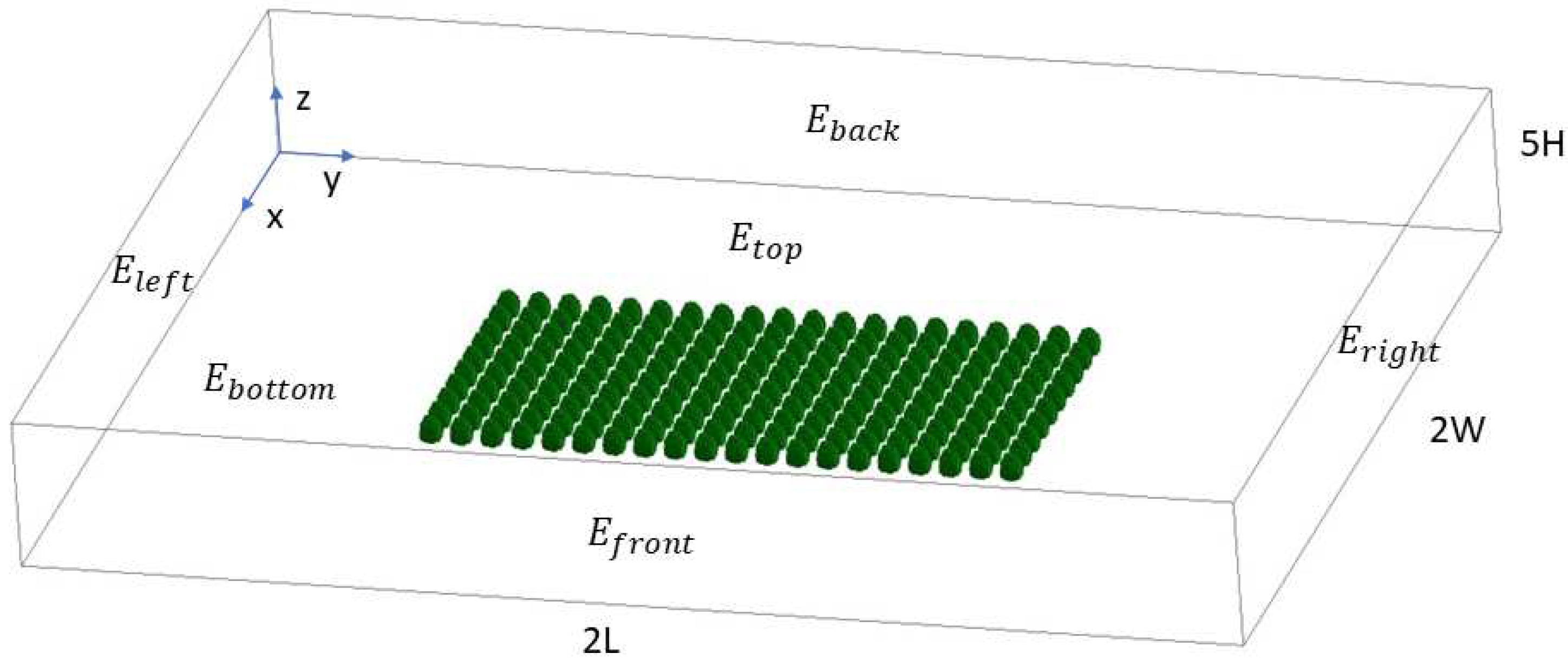
As shown in Figure 3, the computational domain for the fruit orchard is taken as a rectangular prism. The temperature boundary conditions for the ground and the sky are specified as constants, assuming their surfaces are maintained at fixed temperatures during the frost event. Four side boundaries, including left, right, front, and back, are set as an inlets or outlets depending on the wind direction. The temperature boundary condition for the inlet is specified as a logarithmic temperature profile where the temperature at the bottom end (the ground) and at the top end (the sky) are set to T ground and T sky , respectively. The temperature boundary condition for the outlet is set as a no-flux boundary.
With reference to Figure 3, we have the following set of boundary conditions:
T | E b o t t o m = T g r o u n d , T | E t o p = T sky
T | E i n l e t = f ( z ) = c 1 log ( z + 1 ) + c 2
T n | E o u t l e t = ( T · n ) | E o u t l e t = 0 ,
where n denotes the wind direction; E i n l e t and E o u t l e t are the edges associated with the inlet and outlet, respectively; f ( z ) is the temperature profile (K) with respect to the altitude, z; and c 1 and c 2 are constants to satisfy the condition that temperature at the ground and the sky are T ground and T sky , respectively.

2.5. Validity of the Developed Model

The airflow patterns in a fruit orchard induced by external winds and drag effect of tree canopies were validated well by Hong et al. [14,16]. In these studies, air velocity distributions inside and around tree canopies were predicted by CFD simulations integrated with the source terms introduced in Section 2.2 and showed a relative error of 29.2% when the simulation results were compared to field measurements. Considering the high variations of crop characteristics in field conditions, the simulation results were quite reasonable. All details regarding the simulations of airflow patterns can be found in Hong et al. [14]. The same CFD models were also used for SAAS, a computer program for estimating pesticide spray drift from orchards [23]. In the SAAS program, the CFD models predicted canopy air flows according to various fruit types and wind conditions with a reasonable accuracy.
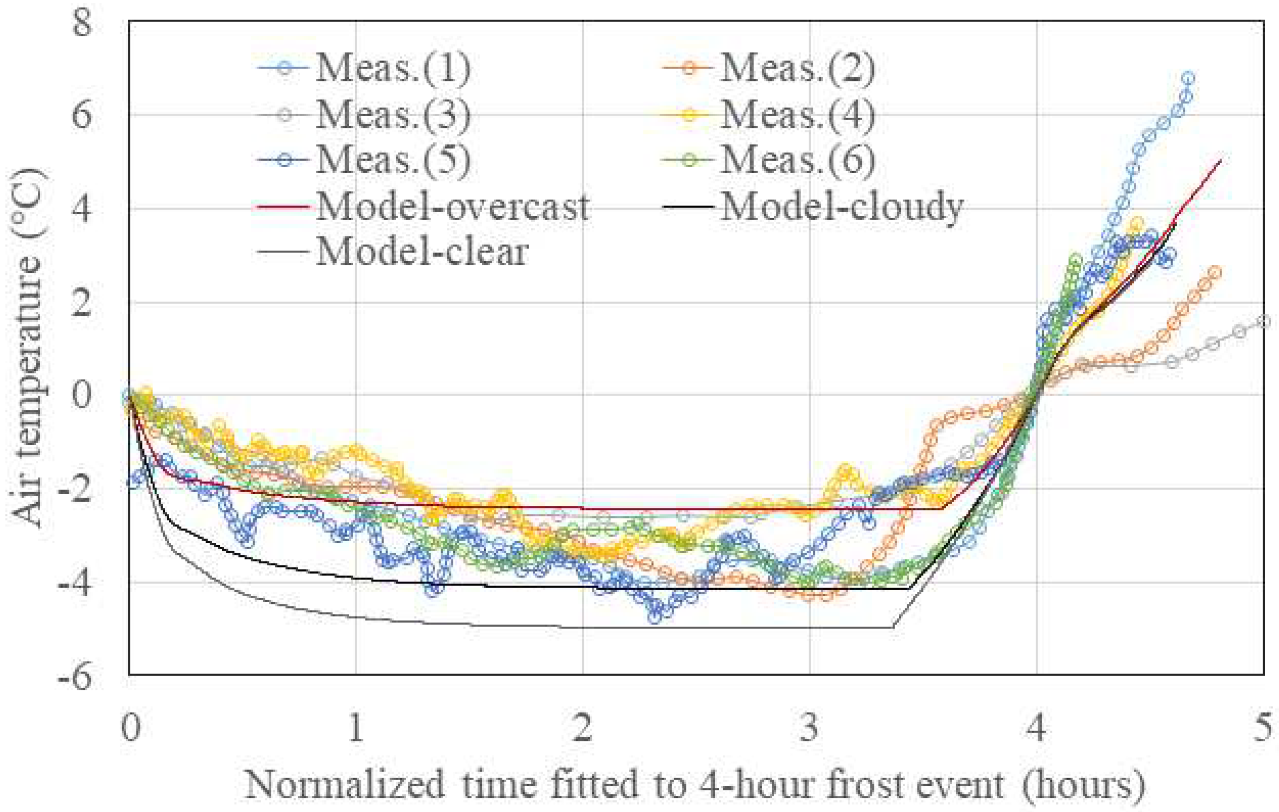
The thermophysics models described in Section 2.3 predicted the temporal variation of air temperature in an orchard. For the validation of the thermophysics models, the air temperature determined by heat exchanges with the canopy, ground, and sky was compared to the field measurements conducted in a peach orchard and an orange orchard by Ghaemi et al. [24]. As shown in Figure 4, the air temperatures in the orchards during six frost events were compared to the CFD simulation results for three frost episodes (mild, medium, and severe frost levels), which are described in detail in the case study given in Section 3. The simulated air temperatures decreased at the beginning of the frost events due to radiative cooling and increased at the end of the frost events due to solar heating. The frost intensity of the six frost events was not determined by Ghaemi et al. [24], and, therefore, the simulated air temperature variations of three frost cases cannot be directly compared with those of the six measured frost events. In Figure 4, some measured air temperatures dropped to the simulated ones of the “clear” (severe) case, while most measured air temperatures ranged between the “overcast” (mild) and “cloudy” (medium) cases. Therefore, we believe that the simulated air temperatures of the three frost events were in the range of real frost events. Although the air temperatures decreased slightly steeply compared to the field measurements, the overall air temperature variations were in good agreement with the actual frost events because in the simulations the temperature drop when the frost occurred and radiation balance at the time of frost were more important than the steep air temperature drop before the frost occurred.

2.6. Parametric CTFD Model Simulation Procedure

The simulation procedure of the parametric CTFD model is as follows. First, we need to set the orchard parameters (fruit type, orchard size, etc.) and boundary/initial conditions (which are considered part of climate data). Second, to run the model we need to specify the operational principle of the control unit of hot air blowers in zones of the fruit orchard (see Figure 1). Here, the controller type we use is a rule-based controller whose operational principle is based on the following rules:
  • For each zone in Figure 1, a separate controller is to be used for controlling blow of heated air on trees. Let us denote the controller for the i-th zone as C i , i = 1 , 2 , , n , where n is the number of zones.
  • Controllers must work independently of each other.
  • Set the control-time step t s (which is the time interval at which a controller provides a fixed control input of either zero heat flux or the possible maximum heat flux to the orchard) to t s = 60 s . In fact, t s can be considered as a “simulation parameter” and can be set to different values depending on the frost scenario. For example, in case of severe frosts t s can be set to lower values, such as to 10 s.
  • In principle, t s can be different for each C i , but better to be the same to simplify the simulation procedure.
  • Let the heat flux provided to each zone by C i be Q i ( t ) with minimum and maximum values of Q min and Q max , respectively. Q min can be set to zero simply and Q max depends on the capacity of air heaters. Let the control period over which to control the orchard be divided into a set of N intervals where the length of each interval is t s . Let us denote the time points at the beginning of each interval by t 1 = 0 < t 2 < t 3 < < t N = ( N 1 ) × t s . Q i ( t k ) , i = 1 , , n , k = 1 , , N , is determined as follows. For zone i at time t k , calculate the average temperature of each tree in the zone and let T i min avg be the minimum of all these calculated average tree temperatures. Then, determine Q i ( t k ) as:
    Q i ( t k ) = 0 , if T i min - avg 0 C Q max , otherwise .

3. Case Study: Use of Parametric CTFD Model for Frost Preventing Energy Calculations

In this section, we demonstrate, among many, one useful application of the developed parametric CTFD model: to calculate the required minimum frost prevention energy for three frost episodes (corresponding to a mild level frost, medium level frost, and severe level frost) for a test on a Prunus armeniaca orchard located in Malatya, Turkey. With reference to Figure 1, the test orchard dimensions are given as L = 200 m , W = 100 m , H = 9 m , s = 10 m , and we assume that there are 10 zones ( n = 10 ). The parameters associated with the Prunus armeniaca tree canopy are given in Table 2.
The three frost episodes have identical conditions except the cloud cover constant because the fraction of the sky obscured by clouds influences the rate of radiative cooling, and thus the degree of frost. The common conditions for the three episodes are the ground temperature ( T g r o u n d ) of −5 C, the upper-boundary temperature ( T s k y ) of 7 C, and air relative humidity of 50%. The boundary condition parameters c 1 and c 2 of the inlet air temperature profile in (15) were determined to be 3.494 and −5.0, respectively. The air temperature and canopy temperature were calculated transiently based on the thermophysical processes. Since a strong wind does not promote the formation of frost, the wind speed in the case study was assumed to be 0.3 m/s at a height of 10 m in the form of the log-law wind profile. The wind blew in + y direction (with reference to Figure 3), and, thus, E l e f t and E r i g h t were set as inlet and outlet, respectively.
The cloud cover constants (C, see Equation (8)) were set to 1.0, 0.6, and 0.0 for mild, medium, and severe-level frost episodes, respectively. The severe frost condition occurs due to extreme radiative cooling for clear sky ( C = 0.0 ), while the mild frost is due to low radiative cooling for a totally overcast sky ( C = 1.0 ). Finally, it is assumed that a frost episode lasts 4 h. The simulation of each such frost event took around 5 days using a computer with an Intel i7-7800X (3.5 GHz) CPU and 64 GB RAM.

Results and Discussions

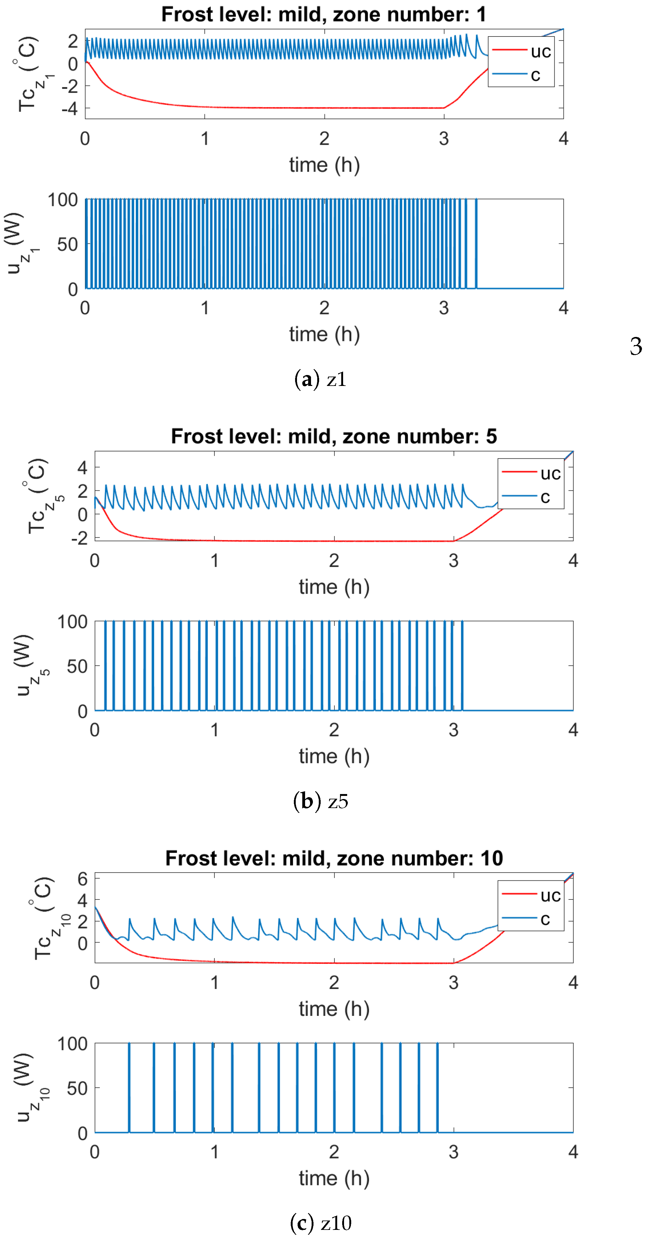
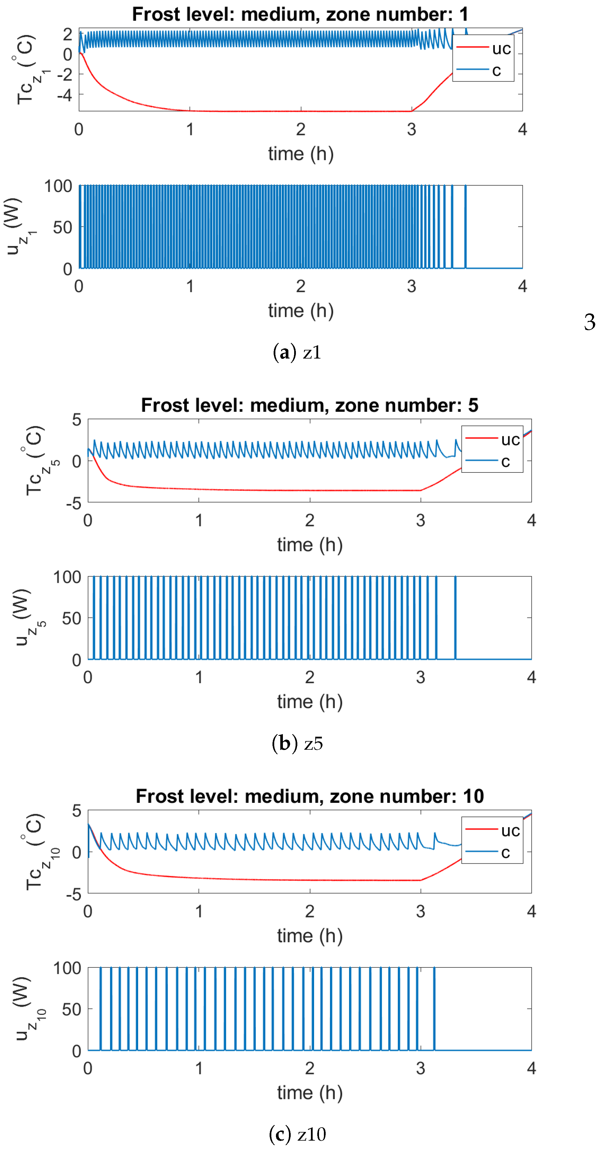
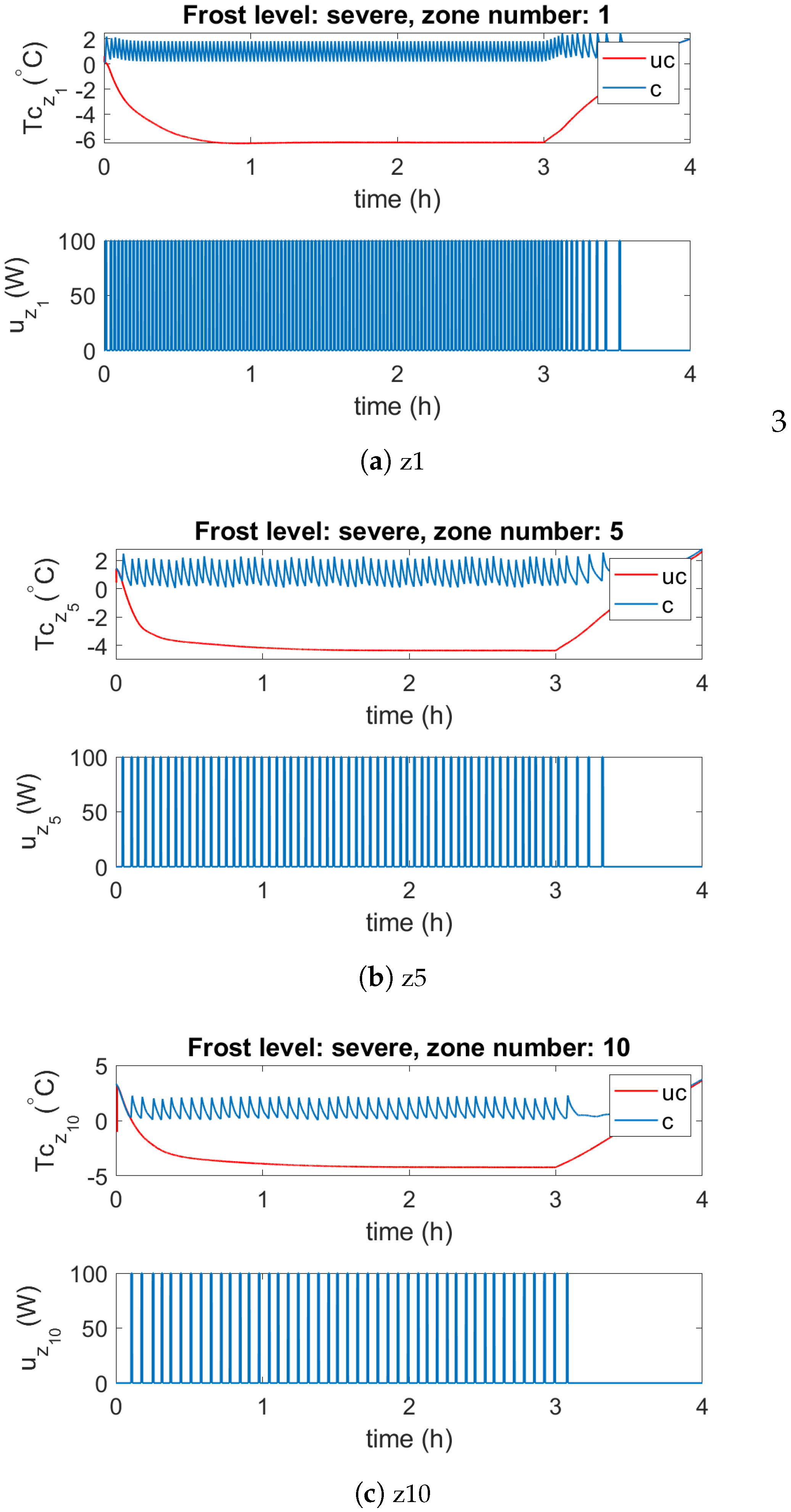
A snapshot showing horizontal spatial temperature variations at the vertical cross section (z = 1.5 m) for each frost episode when no heating is applied (uncontrolled frost case) is given in Figure 5. The simulations results of the uncontrolled orchard and controlled orchard for three frost levels are given through Figure 6, Figure 7 and Figure 8 and Table 3. The results in Figure 6, Figure 7 and Figure 8 show the successful control of the canopy temperature (which is always above 0 C) in the considered three frost episodes. The windward zones, such as zone 1, were more vulnerable to frost than the leeward zones, such as zone 10, and required more frequent operations of hot air blowers than the leeward zones, as shown in Figure 6, Figure 7 and Figure 8. As a result, the heaters were operated approximately six times longer in total in zone 1 and 2 compared to zone 9 and 10, causing more energy demands. The internal zones, such as zones 3-8, needed moderate energy demands compared to the boundary zones, such as the windward and leeward zones. Therefore, considering that wind can blow from any direction, the boundary zones needed more careful concern compared to the internal zones.
The results in Table 3 indicate that the total energy required to prevent frost for a duration of 4 h in a test orchard consisting of 200 trees located in Malatya, Turkey changes in the range 734–1250 kWh, which is not large. Moreover, note that the controlled temperatures in Figure 6, Figure 7 and Figure 8 are obtained through an on-off controller, which can be suboptimal compared to a PID (proportional–integral–derivative) or a model-based controller. As a result, by employing a better controller, the range 734–1250 kWh can be further reduced.

4. Thermofluid Modelling for Optimal Design and Control of Active Frost Prevention Systems Integrating Renewable Energy

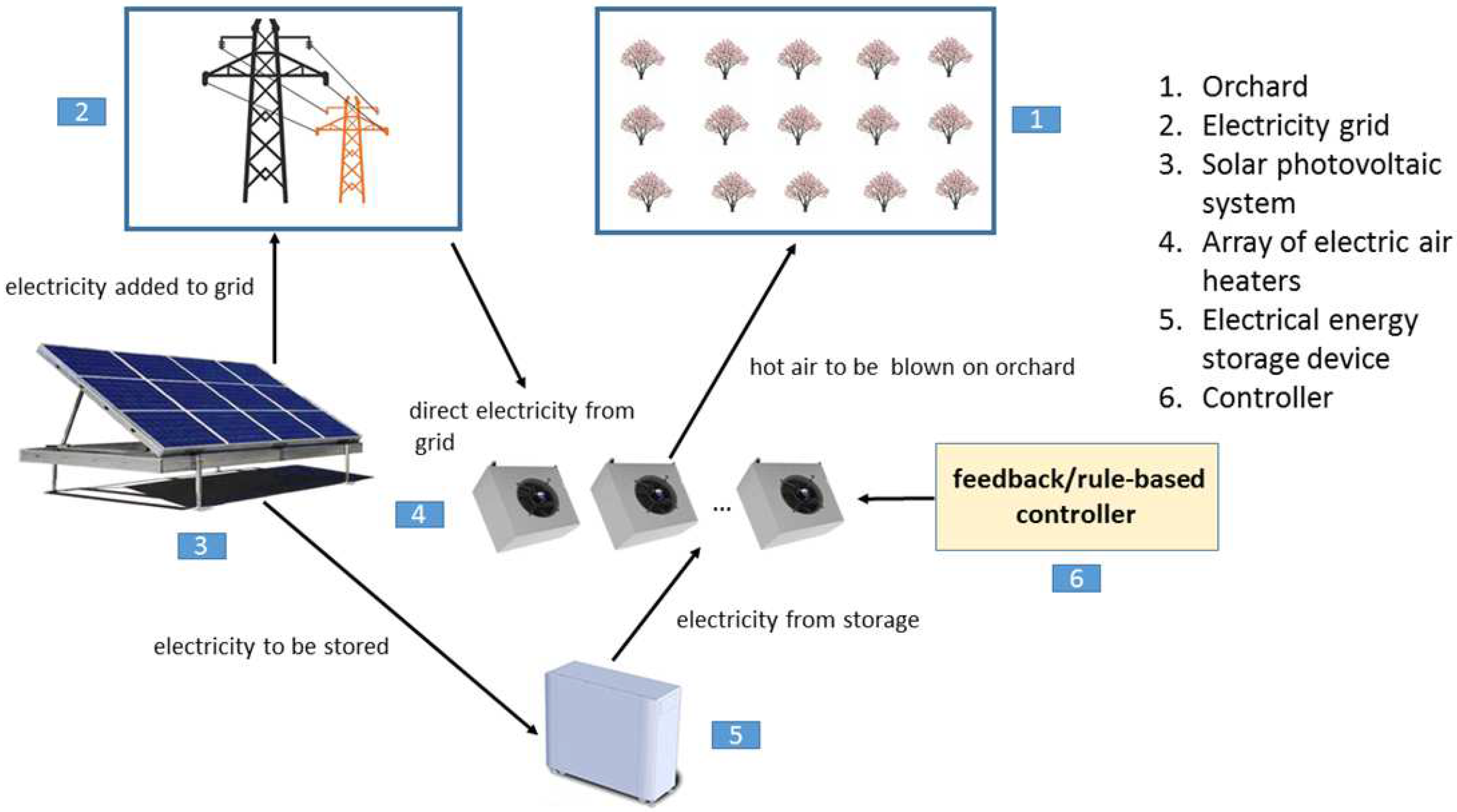
Using the developed parametric CTFD model, we showed in the previous section that the minimum energy required to prevent a frost episode in a test Prunus armeniaca orchard consisting of 200 trees is in the range 734–1250 kWh. Active frost prevention systems integrating renewable energy sources (for example, photovoltaics, solar-thermal, and geothermal) can be designed to partially or fully provide this energy. An example, a photovoltaics-based (PV) system, is illustrated in Figure 9. Here, in the PV-assisted framework, solar energy is used as a secondary application for frost prevention (the primary application is electricity production for the grid). The PV-based system is mainly be used to produce electricity to be added to the grid. It is necessary to store some of the electricity produced when the frost periods approach. The size of storage unit depends on the size of the fruit orchard and the predicted frost level. The electricity from the grid or storage device is used to heat air by an array of electric air heaters where, again, the capacity of heaters in the array depends on the size of the orchard and the frost level. The heated airis blown by fans on fruit trees during freezing days. The frost prevention control system controls the blowing time and the mass flow rate of the heated air. The PV-based frost prevention system is a good choice for regions with a rich solar radiation level.
The framework in Figure 9 is just one possibility among many. For example, solar-thermal, geothermal systems with/without thermal energy storage are also possible. In all such renewable energy-integrating active frost prevention systems, the developed CTFD model can be used extensively for optimal design and control of such a system. For example, using the CTFD model a simulation-based optimisation can be done to optimally size the frost prevention system to minimise the investment cost and payback time, the CTFD model can be used to obtain control-oriented models to design model-based control systems controlling the frost prevention system and to test them before testing on the real system. Optimal control system deign is a must for minimisation of operational costs. As a result, the development of a CTFD model for the air thermal dynamics of large-scale fruit orchards is the key step before frost prevention system optimisation and control.

5. Conclusions and Recommendations

In this paper, a parametric CTFD model was developed for air thermal dynamics simulation of heated fruit orchards. The developed parametric CTFD model can be very useful (i) to determine the required minimal energy to be provided by an active frost prevention energy system for a given orchard; (ii) to optimally size the active frost prevention energy system to minimise the investment cost and payback time; (iii) to develop reduced-order control models for model-based control approaches (such as nonlinear model predictive control) to minimise the operational cost of active frost prevention energy system; and (iv) to test the developed control systems on the parametric CTFD model under different parameters and climates before testing the controller on the real system. The orchard air temperature predictions from the developed CTFD model agreed well with the experimental data from field measurements under similar conditions. The use of developed parametric CTFD model was demonstrated through simulation of the canopy thermal dynamics of a heated test Prunus armeniaca orchard located in Malatya, Turkey, which is the world capital for dry apricot production. This test case considered different frost levels and we calculated the required minimum thermal energy to prevent frost in each case, where a rule-based control system was used to control the operation of hot air blowers. The computation time needed to simulate a frost event lasting 4 h was around 5 days. The calculated energy levels, using the developed parametric CTFD model, showed that frost can be prevented in large-scale orchards at an acceptable operational cost, which is the main conclusion of this study.
There are many other research avenues and/or practical applications to be derived from this study. Some of them can be listed as follows. (i) developing a control-oriented model and using this model to design a nonlinear model predictive control (NMPC) system for frost prevention; (ii) determining the optimal number and distribution of hot air blowers; (iii) development of optimised, rule-based controllers from NMPC-type controllers through machine learning; (iv) consideration of synergistic effects by using hot air blowers and other alternatives, such as water sprayers around the perimeter of the orchard, and mulching or coverage of the fruit trees, which could significantly reduce the required minimum frost prevention energy from the use of hot air blowers; (v) development of different active frost prevention systems, including renewable energy sources and their economic feasibility analyses: for example, photovoltaics systems [25] and ground-coupled heat pumps [26,27,28] to fully or partially heat/warm the hot air to be blown.

Author Contributions

Conceptualization, methodology, simulation, formal analysis, writing, review and editing, E.A. and S.-W.H.; Feedback, A.A. All authors have read and agreed to the published version of the manuscript.

Funding

The first author would like to thank TÜBİTAK for funding (through the TÜBİTAK 1512 program) his project entitled “Development of tools for solar-energy assisted frost prevention systems in large-scale orchards”.

Conflicts of Interest

The authors declare no conflict of interest.

Nomenclature

Acronym/SymbolDescription
CFDComputational fluid dynamics
CTFDComputational thermofluid dynamics
PIDProportional-integral-derivative
RANSReynolds-averaged Navier–Stokes
A c Ground area of the tree canopy
A t Area of the tree stem
CCloud cover constant
C g , t r e e The group of grid cells located within trees
C i r Pressure loss coefficient
C p , c Specific heat of leaves
dTree diameter
ETotal air energy
gGravitational acceleration
hSensible air enthalpy
HHeight of trees
JDiffusion flux
kTurbulent kinetic energy
k e f f Effective air conductivity
LLength of the orchard
L c Characteristic length of leaves
pAir pressure
r leaf - res The aerodynamic resistance of the leaf boundary layer
sDistance between roots of trees
t c Thickness of leaves
uAir velocity
u 0 Buoyancy air velocity
v a Wind speed
P conv c The convective heat exchange between tree canopy and the surrounding air
P ground - cond c Conductive heat flux between the ground and tree canopy
P rad - down c Radiation heat flux from sky to tree canopy
P rad - up c Outgoing radiation from tree canopy
R H Relative humidity
S h Air source term
S s e Sensible heat exchange between the trees and air
S s h Sensible heat generation from heaters inside the orchard
S u Source term for momentum loss due to tree canopies
TAir temperature
T c Canopy temperature
T g Ground temperature
T s Sky temperature
UConductance of the tree stem
wSpecific dissipation rate
WWidth of the orchard
ϵ Emissivity
ρ Air density
ρ c Tree canopy density
μ Air viscosity
μ t Turbulent air viscosity
σ Stefan–Boltzmann constant

References

  1. The Fruit and Vegetable Sector in the EU—A Statistical Overview. 2018. Available online: http://ec.europa.eu/eurostat (accessed on 8 December 2019).
  2. Gunduz, O.; Ceyhan, V.; Bayramoglu, Z. Influence of climatic factors on apricot (Prunus armeniaca L.) yield in the Malatya province of Turkey. Asian J. Agric. Sci. 2011, 3, 150–155. [Google Scholar]
  3. Batmaz, M.F. Studies on Some Apricot Genotypes under Adana Ecological Conditions. Master’s Thesis, Cukurova University, Adana, Turkey, 2005. (In Turkish). [Google Scholar]
  4. Perry, K.B. Basics of frost and freeze protection for horticultural crops. HorthTechnology 1988, 8, 10–15. [Google Scholar] [CrossRef] [Green Version]
  5. De Melo-Abreu, J.P.; Villalobus, F.J.; Mateos, L. Principles of Agronomy for Sustainable Agriculture; Springer: Berlin, Germany, 2016; Chapter 29; pp. 443–457. [Google Scholar]
  6. Avissar, R.; Mahrer, Y. Mapping frost-sentive areas with a three-dimensional local-scale numerical model. Part I: Physical and numerical aspects. J. Appl. Meteorol. 1988, 27, 400–413. [Google Scholar] [CrossRef] [Green Version]
  7. Robinson, C.; Mort, N. A neural network system for the protection of citrus crops from frost damage. Comput. Electron. Agric. 1997, 16, 177–187. [Google Scholar] [CrossRef]
  8. Prabha, T.; Hoogenboom, G. Evaluation of the weather research and forecasting model for two frost events. Comput. Electron. Agric. 2008, 64, 234–247. [Google Scholar] [CrossRef]
  9. Rahimi, M.; Eccel, E. Modelling the effects of meteorological and geographical drivers on damage from late radiation frost on apple trees in Northeast Iran. Ital. J. Agrometeorol. 2016, 3, 13–22. [Google Scholar]
  10. Issa, R.J. Numerical heat transfer model for frost protection of citrus fruits by water from a spraying system. Therm. Sci. 2012, 16, 31–42. [Google Scholar] [CrossRef]
  11. Wu, W.; Hu, Y.; Yang, S.; Mao, K.; Zhu, X.; Li, P. Optimal design of wind machine impeller for frost protection based on CFD and its field test on airflow disturbance. Int. J. Agric. Biol. Eng. 2015, 8, 43–49. [Google Scholar]
  12. Green, R.S. Modelling turbulent air flow in a stand of widely-spaced trees. Phoenics J. 1992, 5, 294–312. [Google Scholar]
  13. Gros, G. Numerical Simulation of Canopy Flows; Springer: Berlin, Germany, 1993; pp. 34–91. [Google Scholar]
  14. Hong, S.W.; Zhao, L.; Zhu, H. CFD simulation of airflow inside tree canopies discharged from air-assisted sprayers. Comput. Electron. Agric. 2018, 149, 121–132. [Google Scholar] [CrossRef]
  15. Bjerg, B.; Cascone, G.; Lee, I.B.; Bartzanas, T.; Norton, T.; Hong, S.W.; Seo, I.H.; Banhazi, T.; Liberati, P.; Marucci, A.; et al. Modelling of ammonia emissions from naturally ventilated livestock buildings. Part 3: CFD modelling. Biosyst. Eng. 2013, 116, 259–275. [Google Scholar] [CrossRef]
  16. Hong, S.W.; Zhao, L.; Zhu, H. CFD simulation of pesticide spray from air-assisted sprayers in an apple orchard: Tree deposition and off-target losses. Atmos. Environ. 2018, 175, 109–119. [Google Scholar] [CrossRef]
  17. Tennekes, H.; Lumley, J.L. A First Course in Turbulence; The MIT Press: Cambridge, MA, USA; London, UK, 1972. [Google Scholar]
  18. Ansys, Inc. ANSYS Fluent 18 Theory Guide; Ansys, Inc.: Canonsburg, PA, USA, 2017. [Google Scholar]
  19. Goforth, M.A.; Gilcrest, G.W.; Sirianni, J.D. Cloud effects on thermal downwelling sky radiance. Proc. SPIE 2002, 4710, 203–213. [Google Scholar]
  20. Swinbank, W.C. Long-wave radiation from clear skies. Q. J. R. Meteorol. Soc. 1963, 89, 339–348. [Google Scholar] [CrossRef]
  21. Roy, J.C.; Boulard, T.; Kittas, C.; Wang, S. Convective and ventilation transfers in greenhouses, Part 1: The greenhouse considered as a perfectly stirred tank. Biosyst. Eng. 2002, 83, 1–20. [Google Scholar] [CrossRef] [Green Version]
  22. Jayalakshmy, M.S.; Philip, J. Thermophysical properties of plant leaves and their influence on the environment temperature. Int. J. Thermophys. 2010, 31, 2295–2304. [Google Scholar] [CrossRef]
  23. Hong, S.W.; Zhao, L.; Zhu, H. SAAS: A computer program for estimating pesticide spray efficiency and drift of air-assisted pesticide applications. Comput. Electron. Agric. 2018, 155, 58–68. [Google Scholar] [CrossRef]
  24. Ghaemi, A.A.; Rafiee, M.R.; Sepaskhah, A.R. Tree-temperature monitoring for frost protection of orchards in semi-arid regions using sprinkler irrigation. Agric. Sci. China 2009, 8, 98–107. [Google Scholar] [CrossRef]
  25. Atam, E.; Arteconi, A. Green energy-assisted frost prevention: A conceptual framework. Energy Procedia 2017, 141, 155–159. [Google Scholar] [CrossRef]
  26. Atam, E.; Helsen, L. Ground-coupled heat pumps: Part 1—Literature review and research challenges in modeling and optimal control. Renew. Sustain. Energy Rev. 2016, 54, 1653–1667. [Google Scholar] [CrossRef]
  27. Atam, E.; Helsen, L. Ground-coupled heat pumps: Part 2—Literature review and research challenges in optimal design. Renew. Sustain. Energy Rev. 2016, 54, 1668–1684. [Google Scholar] [CrossRef]
  28. Atam, E.; Patteeuw, D.; Antonov, S.P.; Helsen, L. Optimal control approaches for analysis of energy use minimization of hybrid ground-coupled heat pump systems. IEEE Trans. Control. Syst. Technol. 2016, 24, 525–540. [Google Scholar] [CrossRef]
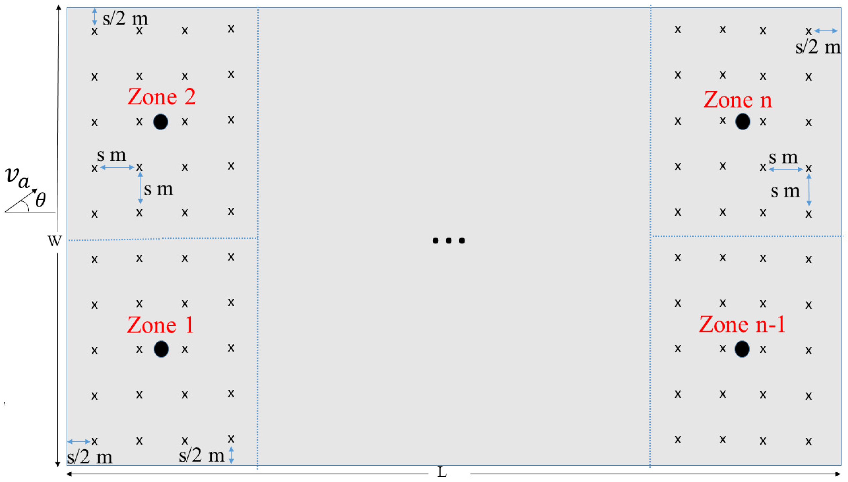
Figure 1. Two dimensional domain for a generic rectangular prism type fruit orchard. Here, “x” denotes trees, “●” hot air blowers, v a the wind speed, and θ wind direction.
Energies 13 00378 g001
Figure 2. Energy flows around trees in a fruit orchard.
Energies 13 00378 g002
Figure 3. Computational domain for the three dimensional rectangular prism-type orchard.
Energies 13 00378 g003
Figure 4. Comparison of air temperature simulation results of parametric CTFD model and field measurements from study [24].
Energies 13 00378 g004
Figure 5. Horizontal temperature variation contours (uncontrolled case) for the considered frost episodes at a height of 1.5 m.
Energies 13 00378 g005
Figure 6. Mild frost canopy temperature simulation results for selected zones z 1 , z 5 , and z 10 . Here, “uc” and “c” denote uncontrolled and controlled cases, respectively.
Energies 13 00378 g006
Figure 7. Medium frost canopy temperature simulation results for selected zones z 1 , z 5 , and z 10 . Here, “uc” and “c” denote uncontrolled and controlled cases, respectively.
Energies 13 00378 g007
Figure 8. Severe frost canopy temperature simulation results for selected zones z 1 , z 5 , and z 10 . Here, “uc” and “c” denote uncontrolled and controlled cases, respectively.
Energies 13 00378 g008
Figure 9. PV-integrated frost prevention system schematics.
Energies 13 00378 g009
Table 1. Physical parameters associated with the canopy of a fruit orchard modelled by a parametric CTFD model. The leaf area index is the total one-sided leaf area per the ground area occupied by the plant, while the leaf area density is the total leaf area per plant-occupied volume. The leaf characteristic dimension is a equivalent circular area diameter.
Variable DescriptionVariable Notation
Canopy width (m) w canopy
Tree height (m) h tree
Trunk diameter (m) d trunk
Trunk height (m) h trunk
Leaf area index ( m 2 × m 2 ) L AI
Leaf area density ( m 2 × m 3 ) L AD
Leaf characteristic dimension (m) L CD
Table 2. Physical characteristics of apricot trees modelled in CTFD model.
VariablesValues
Canopy width (m)6.0
Tree height (m)9.0
Trunk diameter (m)0.4
Trunk height (m)1.5
Leaf area index ( m 2 × m 2 )3.0
Leaf area density ( m 2 × m 3 )2.0
Leaf characteristic dimension (m)0.1
Table 3. Active heater operation times and required minimum energy to prevent frost under three frost scenarios.
Frost ConditionSky ConditionActive Heater Operation Times
z1z2z3z4z5z6z7z8z9z10Total
Mild frostOvercast484822222121111188220
Medium frostCloudy65653232292920211818329
Severe frostClear67673838343426262323376
Frost ConditionSky ConditionEnergy Demand of Each Zone (kWh) [Heating Rate Was 100W/ m 2 ]
z1z2z3z4z5z6z7z8z9z10Total
Mild frostOvercast1601607272717136362828734
Medium frostCloudy2172171071079696676960601096
Severe frostClear222222127127112112868678781250