Abstract
The state of health (SOH) and remaining useful life (RUL) of lithium-ion batteries are two important factors which are normally predicted using the battery capacity. However, it is difficult to directly measure the capacity of lithium-ion batteries for online applications. In this paper, indirect health indicators (IHIs) are extracted from the curves of voltage, current, and temperature in the process of charging and discharging lithium-ion batteries, which respond to the battery capacity degradation process. A few reasonable indicators are selected as the inputs of SOH prediction by the grey relation analysis method. The short-term SOH prediction is carried out by combining the Gaussian process regression (GPR) method with probability predictions. Then, considering that there is a certain mapping relationship between SOH and RUL, three IHIs and the present SOH value are utilized to predict RUL of lithium-ion batteries through the GPR model. The results show that the proposed method has high prediction accuracy.
1. Introduction
Lithium-ion batteries are the core power sources for electric vehicles (EVs), consumer electronics, and even spacecraft, etc. [1,2,3]. Therefore, the reliability and safety of lithium-ion batteries is a critical problem in the process of actual applications. The performance of batteries gradually deteriorates with the increase of service life, which might not only affect the normal operation of electrical equipment, but also bring about serious consequences [4]. For example, there was the cell explosion of the Samsung NOTE7, the spontaneous combustion of electric vehicles, and the explosion of battery energy storage boxes in some power plants in recent years [5].
In order to avoid such accidents, SOH and RUL prediction of lithium-ion batteries has become a hotspot and challenging subject in the prognostics and health management (PHM) of electronics. In fact, the battery management system (BMS) is designed for various instruments to ensure safe operating conditions. SOH determination and RUL prediction are the key functions of BMS in current practice. They need to be estimated using online measurement data including current, voltage, and temperature, etc.
The existing methods for SOH and RUL prediction of lithium-ion batteries can be roughly divided into two main categories: model-based approaches and data-driven approaches [6]. The electrochemical model (EChM) and the equivalent circuit model are two common models. The most popular EChM is Doyle–Fuller–Newman (DFN) model [7,8,9]. Safari et al. [10] developed a multimodal physics-based aging model for the capacity fade of the lithium-ion batteries. The model combined the solvent decomposition kinetics and solvent diffusion through the solid electrolyte interphase (SEI) layer. Considering desolvation as a rate-limiting step, in Ref. [11,12], the authors used a one-dimensional model to estimate the aging of the battery by considering both the calendar and cycle phenomena together [13]. Although the model has high simulation accuracy, it is very complicated to simulate in online applications. Thus, model reduction methods are used to reduce the order of these models. Ramadesigan et al. [14] employed reformulated models to efficiently extract the effective kinetic and transport parameters from experimental data. An alternative approach, using voltage-discharge curves measured during initial cycles to predict voltage-discharge curves during later cycles, is analyzed. Ashwin et al. [15] proposed a pseudo-two-dimensional electrochemical lithium-ion battery model to study capacity degradation under cyclic charging and discharging conditions, but this model was largely unable to achieve dynamic tracking, so its accuracy was poor. The major drawback of this method is that the reduction models are obtained under certain conditions, which will limit the achievable accuracy and introduce modeling errors.
Equivalent circuit models are less complicated than EChM, and are easy to implement for real-time applications with medium accuracy. Johnson et al. [16] developed two classical equivalent circuit models: the battery internal resistance equivalent (Rint) model and the impedance resistance–capacitance (RC) model. Although the implementation of the equivalent circuit model was strong, it was easy to ignore the implicit relationship between the internal state variables of the battery. In Ref. [17], the simplest Thevenin model with one RC branch is presented, and all the model parameters are constant. When equivalent circuit models are used to estimate battery aging, model parameters include lots of internal battery parameters and resistance aging parameters. Parameter identification requires a large and diverse data set obtained with time-consuming tests. However, due to the incomplete understanding of the capacity degradation mechanism of lithium-ion batteries, it is difficult to determine the main parameters involved in the model-based method. Some parameters of side reactions accompanying the main reaction are also difficult to determine through parameter identification. Moreover, model-based methods exhibit poor real-time performance.
With the rapid development of machine learning and artificial intelligence, data-driven methods have been receiving more and more attention [18,19,20]. In addition, a large number of performance data of lithium-ion batteries can be obtained from actual applications. This provides the foundation for applying data-driven methods to predict the aging life of lithium-ion batteries. Compared with the model-based methods, data-driven methods are nonparametric, and do not consider the electrochemical principles to some extent. Thus, degradation models of lithium-ion batteries are developed with various mapping and regression tools.
Existing approaches include time series analysis, artificial neural network (ANN), support vector machine (SVM), relevance vector machine (RVM), Gaussian process regression (GPR), and so on. Long et al. [21] applied an improved autoregressive (AR) model by particle swarm optimization (PSO) to make online predictions. The calculation of the AR model was simple, but the prediction results did not have an uncertain expression of the results. Andre et al. [22] used a structured neural network algorithm to reduce the complexity of network structure and improve the calculation speed, but the prediction results only gave point estimates. The prediction performance was poor when the number of samples was small. Gao et al. [23] proposed a multikernel SVM (MSVM) based on polynomial kernel and radial basis kernel function to predict RUL of the battery. But SVM easily suffered from the local optimum because of its characteristics.
In recent years, the GPR method has been favored by researchers because it is a probability prediction model under the Bayesian framework [24,25]. In order to realize multiple-step-ahead prognostics, Liu et al. [26] utilized an improved GPR model-combination Gaussian Process Functional Regression (GPFR) to capture the actual trend of SOH, including global capacity degradation and local regeneration. Although it had certain advantages in long-term predictions, the capacity was selected as the degradation data, which had some limitations for practical applications. In Ref. [27], Peng et al. proposed a fusion method of the wavelet denoising (WD) method and the GPFR model base on that of Liu et al. [26], where the WD was applied to remove the noise from the original data; the GPFR model was then employed to obtain higher accuracy RUL predictions. The prediction of RUL was improved, but the method only focused on the degradation trend of batteries, and ignored the regeneration phenomenon in battery rest life. Empirical mode decomposition (EMD) was used to extract global tendency and local fluctuations in the battery SOH series, which reduced the affection of the local regenerations in the battery charge procedure [28]. The multiscale logistic regression (LR) and GPR were further constructed for modeling the global tendency and local fluctuations, respectively. This method took battery capacity recovery into account, but indirect health indicators with more practical significance were not used for prediction. Generally speaking, some of the above methods use capacity degradation series or impendence to predict SOH and RUL. However, since measuring the impedance and the resistance is time-consuming, it is difficult to make online measurements using the capacity fade data to estimate SOH and RUL [28].
Therefore, some researchers have applied indirect features to substitute capacity data. These can be measured easily in real-time and online, including current, voltage, and temperature, etc. Compared with Ref. [26,27,28], Yang et al. [29] extracted four specific parameters from charging curves, and used them as an input of the GPR model instead of cycle numbers. This method was more meaningful in practical application, but by considering only the charging process voltage change curve, some parameters showed low correlation with capacity, which resulted in reduced prediction accuracy. The discharge process of lithium-ion batteries also plays an important role in aging life prediction. Therefore, to overcome the capacity unmeasurable problem in this paper, we will extract measurable degradation indicators from the charge and discharge process of lithium-ion batteries, which are highly relevant to the capacity fade. The main contribution of this paper is that the proposed method can predict the short-term SOH and long-term RUL of lithium-ion batteries with indirect health indicators (IHIs) and the GPR model. Firstly, in order to reduce the cost of the prediction method and improve the prediction accuracy, this paper proposes to extract indirect health indicators from the data that can be collected by ordinary sensors, such as voltage, current, temperature curves. Then, IHIs with high correlation with the capacity degradation curve are chosen as high-dimensional input by means of grey relation analysis, and the GPR model is developed to predict the short-term SOH of lithium-ion batteries. Finally, considering that there is a certain mapping relationship between SOH and RUL, three IHIs and the present SOH value are utilized to predict RUL of lithium-ion batteries through the GPR model.
The paper is organized as follows. The selection and extraction of IHIs are briefly introduced in Section 2. Section 3 discusses the prediction method based on Gaussian process regression. The simulation results of SOH and RUL are reported in Section 4. Finally, the conclusions are presented in Section 5.
2. Extraction of Indirect Health Indicators
2.1. Experimental Data
The lithium-ion batteries data set used in this paper is from the open data set of NASA Ames Prognostics Center of Excellence (PCoE) [30]. A set of experimental data of lithium-ion batteries including four lithium-ion batteries (Nos. 5, 6, 7, and 18) are used. They are charged and discharged, and the impedance measured under different operating conditions at room temperature (24 °C). The charging process was divided into two steps. The first step was to use 1.5 A constant current charging until the battery voltage reached 4.2 V. The second step was to use constant voltage charging to keep the battery voltage at 4.2 V and reduce the current to 20 mA. The discharging process was carried out under continued current 2 A until the voltage of Nos. 5, 6, 7, and 18 dropped to 2.7 V, 2.5 V, 2.2 V, and 2.5 V, respectively. The capacity degradation curve of each battery is shown in Figure 1.

Figure 1.
Capacity degradation curves of batteries.
2.2. Extraction of Indirect Health Indicators
The capacity of lithium-ion batteries is usually obtained by measuring their internal resistance to reflect the specific capacity [31]. This is because the impedance of the battery increases with the loss of battery life and capacity. But the condition of impedance measurement by impedance meter is harsh and time-consuming [32,33]. Therefore, it is more reasonable to estimate the SOH and RUL of lithium-ion batteries by using common sensors to measure some indirect parameters which are easy to obtain [34].
In this paper, IHIs reflecting the capacity of lithium-ion batteries are extracted from the charge and discharge voltage, current, and temperature curves. The discharge process voltage of lithium-ion batteries with different cycles is shown in Figure 2. It can be seen that the time needed to reach the lowest discharge point (named IHI1) decreases with the increase of cycle numbers, and the time decrement from 3.8 V to 3.5 V (named IHI3) is also shortened. The discharge temperature of lithium-ion batteries with different cycles is shown in Figure 3. When the battery temperature rises to the highest point (named IHI2), the time decreases with the increase of the number of cycles. Moreover, the research shows that the following five indicators can also be used as IHIs: IHI4 is the initial maximum slope of the voltage characteristic curve in the process of discharge; IHI5 is the time when the battery temperature reaches the peak value; IHI6 is the initial maximum curvature of the current curve in the process of constant voltage charging; IHI7 is the charging time; and IHI8 is the area under the current curve.
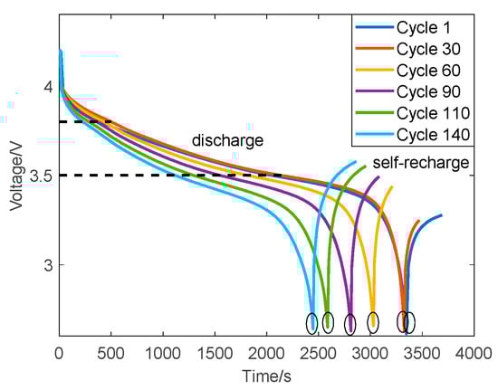
Figure 2.
Discharging voltage curves of No. 5 with different cycles.

Figure 3.
Discharging temperature curves of No. 5 with different cycles.
2.3. Grey Relational Analysis
The similarity between the development trend of the comparison sequence and the reference sequence is analyzed and compared with grey relational analysis (GRA) [35]. In this paper, eight IHIs are extracted as comparison sequences and a capacity degradation curve as the reference sequence. In order to avoid the validity and redundancy of the input eigenvectors, three IHIs with a high correlation degree are chosen as the final health indicators through GRA.
The steps of comprehensive evaluation using GRA are as follows:
Step 1 Make each group of comparative sequence data to form the following matrix:
where is the number of comparison sequences and is the number of data in each comparison sequence, where:
Step 2 Determine the reference data sequence :
Step 3 Calculate the difference of position elements corresponding to each comparison sequence and reference sequence one by one: , where ; .
Step 4 Determine the minimum difference and the maximum difference, and mark the minimum difference as and the maximum difference as .
Step 5 According to Formula (4), the correlation coefficients of location elements corresponding to each comparison sequence and reference sequence are calculated.
where and is resolution coefficients, and in general.
Step 6 Calculate the correlation degree:
For each comparison sequence, the mean value of the correlation coefficients corresponding to the reference sequence is calculated by Formula (5). The calculation result reflects the correlation degree between each comparison sequence and the reference sequence. The closer the value is to 1, the stronger the correlation.
Through a grey relation analysis of eight IHIs, the correlation coefficients between each IHI and the capacity degradation curve was obtained. Based on the results of batteries Nos. 5, 6, 7, and 18, the specific values of the eight IHIs are given in Table 1.

Table 1.
Grey relation grades between IHIs and the battery capacity.
As shown in Table 1, the mean value of the correlation coefficients of IHI1, IHI2, and IHI3 are greater than 0.9, whereas those of the other five IHIs are less than 0.9. There is a good correlation between the battery capacity and the three IHIs. Therefore, these IHIs can be used to replace the capacity to predict the SOH and RUL of the battery.
3. Method
3.1. Gaussian Process Regression
GPR is a nonparametric model based on Bayesian theory. Its output variables are uncertain [36]. A core idea is to regard the random process composed of multiple random variables as a high-dimensional joint normal distribution [37].
A typical GPR is used to approximate the target output f(x), where is the d-dimension input vector and the output function f(x) is the probability distribution:
where and are mean and covariance functions respectively. Considering the linear decline of battery capacity degradation trend in the Gaussian prediction model, the linear function is used as the mean value function, as in Formula (6); At the same time, we choose the squared exponential covariance function (SE), as in Formula (7):
For many real scenes, the observation output can be expressed as an implicit function, that is,
where is the observation vector , is the Gaussian noise and . Therefore, the prior distribution of observations is as follows:
where is an n-dimensional unit matrix and is a noise covariance matrix. is a symmetric positive definite matrix, which can be expressed as:
The similarity of variables and can be determined by Equation (11). The greater the similarity between the two variables, the greater the value of . According to the derivation process, the corresponding values can be obtained by optimizing the negative log marginal likelihood () as
is expressed as follows:
Equation (13) can be solved by using an effective gradient descent algorithm. The basic idea of the algorithm is to get the maximum value of the objective function by calculating the derivative of the log-likelihood function.
where is the element that sets the super parameter. By using the above calculation process, the GPR model is completed. Then, the GPR model is used to predict the task through posterior distribution. Because GP is a random process, the new input dataset follows the Gaussian distribution of the training dataset . Therefore, the joint prior distribution of the observed value and the predicted value at the predicted point are expressed as:
Considering the joint Gaussian prior distribution on , the posterior distribution is analytically derived as:
where the prediction mean and the prediction covariance are given as follows:
Here the mean prediction values are taken as the prediction value of the test datasets, and the covariance prediction values are used to reflect the uncertainty of the GPR model.
3.2. Overall Prediction Process
The indirect prediction process of SOH and RUL of lithium-ion batteries based on GPR is divided into the following seven steps:
Step 1 Extract data:
In the data set provided by NASA, the capacity data set C is collected, and the data sets of eight IHIs are extracted and collated, and recorded as H1~H8.
where is the capacity value corresponding to the number of cycles , and is the mth indirect indicator value corresponding to the ith cycle. ( is the number of cycles); .
Step 2 IHIs are selected by grey relation analysis:
Taking H1~H8 as the comparison sequence of each group and as the reference sequence, three IHIs with the highest correlation degree are determined as the input through the grey relation analysis and marked as .
Step 3 Data preprocessing:
Convert capacity series to SOH series:
Three selected IHIs are normalized:
Step 4 Construct the training set and test set of SOH prediction:
Record the training set predicted by SOH as , the test set as , and the number of cycles corresponding to the predicted starting position as .
Step 5 Training and prediction of SOH prediction model:
Put into the GPR model, and determine the SOH prediction model .
The prediction part will be used as input to get the prediction value .
where is the confidence intervals (CI) for the SOH prediction.
Step 6 Construct the training set and test set of RUL prediction:
Record the training set predicted by RUL as , the test set as , and the number of cycles corresponding to the predicted starting position as .
where is the number of cycles when the battery reaches the failure threshold.
Step 7 Training and prediction of RUL prediction model:
Put into the Gaussian process regression model, and determine the RUL prediction model .
The prediction part will be used as input to get the prediction value .
where is the confidence intervals (CI) for the RUL prediction.
Four indicators are used to evaluate quantitatively the performance of the proposed method: the mean absolute percentage error (MAPE) of SOH, the root mean square error (RMSE) of SOH, the absolute error (AE) of RUL, and the mean absolute error (MAE) of RUL.
The implementation flowchart of the proposed approach is illustrated in Figure 4.
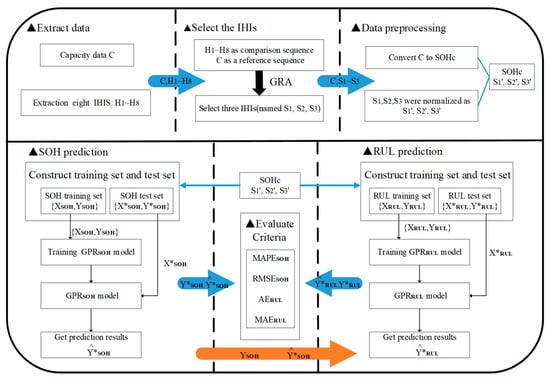
Figure 4.
Schematic diagram of the proposed GPR method for prediction.
4. Experimental Analysis
4.1. SOH Prediction
The feasibility of the proposed SOH prediction model is verified through comparative experiments. The specific meaning of various prediction methods is shown in Table 2. Model M1 uses the number of cycles as input data without using three IHIs; model M2 uses IHIs as input data without using a linear function as the mean function. In this comparison, M1 is tested to analyze the effect of IHIs in the proposed model M3. M2 is considered to illustrate the ability to use a linear function as the mean function. Experimental setting: select the data from cycle 1 to cycle 50 as the training set; the prediction starting point (SP) is 51.
Table 2.
Prediction models used in comparative experiments.
The comparison test results of batteries Nos. 5, 6, 7 and 18 are shown in Figure 5. In order to more accurately reflect the feasibility of the proposed method, the MAPE and RMSE values are shown in Figure 6. It can be observed that the prediction curve of model M3 is the closest to the real capacity degradation curve. Compared with model M3, the prediction result of model M1 is quite different from the real capacity, and it can’t reflect the nonlinear characteristics of capacity degradation. Comparative experiments show that using three IHIs as input data can solve the nonlinear characteristics of capacity degradation. Meanwhile, model M2 uses the IHIs as input data, but the prediction curve is farther away from the real capacity with the increase in cycle numbers. This phenomenon indicates that the GPR without using a linear function as the mean function fails to represent of the overall degradation trend. However, the model M3 has a good prediction performance for capturing the overall degradation trend and tracking the local nonlinear changes.

Figure 5.
Prediction results of comparative experiments: (a) battery No. 5; (b) battery No. 6; (c) battery No. 7; (d) battery No. 18.
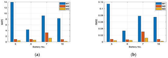
Figure 6.
MAPE and RMSE values in comparison experiments: (a) MAPE; (b) RMSE.
To further verify the feasibility of the proposed model M3, this paper selects the cycle point in the middle and late period as the prediction SP. The prediction results of batteries Nos. 5, 6, 7, and 18 are shown in Figure 7, Figure 8, Figure 9 and Figure 10, where (a) and (b) indicate that the prediction SP is 71 and 91, respectively. It can be observed that the predicted curves of batteries Nos. 5, 6, and 18 at prediction SP = 71 and SP = 91 are close to the real SOH; for battery No. 7, the later the prediction SP, the closer the prediction result to the real SOH.
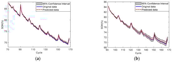
Figure 7.
SOH prediction results of battery No. 5: (a) SP = 71; (b) SP = 91.
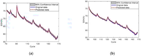
Figure 8.
SOH prediction results of battery No. 6: (a) SP = 71; (b) SP = 91.
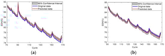
Figure 9.
SOH prediction results of battery No. 7: (a) SP = 71; (b) SP = 91.
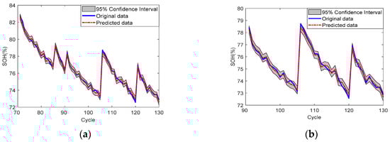
Figure 10.
SOH prediction results of battery No. 18: (a) SP = 71; (b) SP = 91.
Table 3 gives the prediction performance for each battery with different prediction SP. From the experimental results, it can be seen that the proposed model is less affected by the prediction SP in the middle and later stages, and that the prediction accuracy of each battery starting from the middle stage has reached a satisfactory effect. Because the initial experiment is based on battery No. 5, the prediction result of that battery is the best. The prediction effect of batteries Nos. 6 and 18 is not affected by the prediction SP from the middle stage, which reflects that the proposed model has a certain robustness after the middle stage of the prediction SP. However, the performance degradation of battery No. 7 is different from those of the other batteries, which degenerate to about 70% of their original capacities, while battery No. 7 only degenerates to 80%. So, the effect is slightly reduced, but it is also satisfactory, which shows that the proposed model has a good universality for the same kind of batteries.
Table 3.
Prediction performance at different prediction SP of each battery.
In order to prove the accuracy of SOH prediction model M3 proposed in this paper, a method described in [20] is introduced for comparison. A GPR combined with four IHIs from charging curves (named GPR-CF) was proposed in [29], where batteries Nos. 5, 6 and 7 were used, and the prediction SP was set to 81. In order to compare with the model in [29], experiments with model M3 at prediction SP = 81 were designed; the comparison results are shown in Table 4. It can be seen from the results that the accuracy of the proposed method M3 is at least 52.56% higher than the model GPR-CF in Ref. [29].
Table 4.
Comparison of different SOH prediction models for three batteries.
4.2. RUL Prediction
There is a certain mapping relationship between RUL and SOH of lithium-ion batteries, and SOH can be mapped with IHIs. Therefore, three IHIs and present SOH values are used to predict the RUL of lithium-ion batteries through the GPR model.
The end of life (EOL) cycle of lithium-ion batteries is set according to the cycle point corresponding to the battery capacity degradation to the failure threshold. The capacity failure threshold for batteries Nos. 5, 6, and 18 is 1.38 Ah. So, the EOL cycle of each battery is 129,113 and 100, respectively. Since the degradation of battery No. 7 did not reach the failure threshold, no research was done thereon for the time being [38].
The RUL prediction results of batteries Nos. 5, 6, and 18 are shown in Figure 11, Figure 12 and Figure 13, when the prediction SP was selected as 51. Figure 11a presents the RUL prediction results, and 11b the absolute error (AE) of RUL prediction. It can be seen that a slight deviation occurred between the RUL prediction curve and the real RUL curve, but that it remained within a certain range. For battery No. 5, the AE value of each cycle was less than or equal to 23. For batteries Nos. 6 and 18, the AE value of each cycle was less than or equal to 14 and 12, respectively.
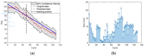
Figure 11.
RUL prediction results for battery No. 5 with SP = 51: (a) RUL; (b) RUL prediction Error.
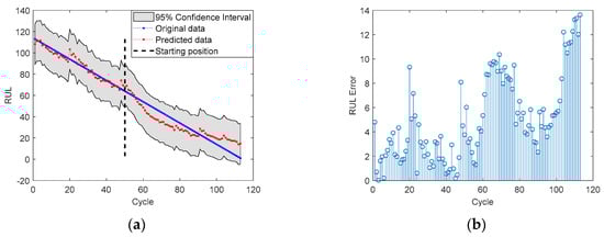
Figure 12.
RUL prediction results for battery No. 6 with SP = 51: (a) RUL; (b) RUL prediction Error.
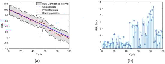
Figure 13.
RUL prediction results for battery No. 18 with SP = 51: (a) RUL; (b) RUL prediction Error.
Considering that the input of the RUL prediction model used the predicted SOH value as one of the inputs, from Table 3, it can be seen that the prediction SP is 71, and the prediction performance has improved significantly. Therefore, it is necessary to observe the performance of RUL prediction when the prediction SP is set to 71.
The prediction results of batteries Nos. 5, 6, and 18 are shown in Figure 14, Figure 15 and Figure 16 when the prediction SP was selected in the medium-term prediction. Figure 14a shows the RUL prediction results, and 14b the AE of RUL prediction. Compared with the prediction results of RUL with the prediction SP of 51, the AE values of batteries Nos. 5 and 18 decreased from not more than 23 and 12 to not more than 8, even though the two abnormal values of battery No. 5 also decreased to 14 and 12. For battery No.6, although the AE value was still in the range of 14 values, the prediction effect of 20 steps after the beginning of prediction was significantly improved.
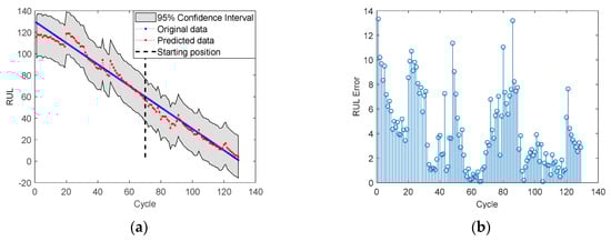
Figure 14.
RUL prediction results for battery No. 5 with SP = 71: (a) RUL; (b) RUL prediction Error.
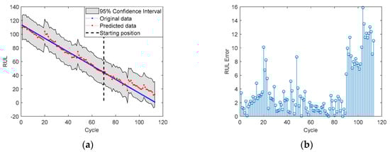
Figure 15.
RUL prediction results for battery No. 6 with SP = 71: (a) RUL; (b) RUL prediction Error.
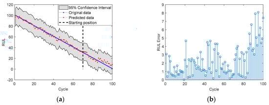
Figure 16.
RUL prediction results for battery No. 18 with SP = 71: (a) RUL; (b) RUL prediction Error.
The mean absolute errors (MAE) of RUL prediction are listed in Table 5. It can be observed that the MAE values with SP = 71 are better than those with SP = 51. Combined with the practical significance of RUL, it is suggested that RUL be predicted in the middle stage of lithium-ion battery life.
Table 5.
The MAE of RUL prediction at different prediction SP for each battery.
Multiscale logistic regression (LR) and GPR were constructed for the model (named MLR-GPR) in Ref. [28], where batteries Nos. 5, 6, and 18 were used. In order to compare with the MLR-GPR model, the prediction SP of RUL prediction model (named IHIs-GPR) proposed in this paper was set to 50, 60, 70, 80, and 90, and AE values were calculated for comparison. The AE value with different RUL prediction models for batteries Nos. 5, 6, and18 are shown in Table 6. It can be seen that the AE of IHIs-GPR was at least 50% less than that of MLR-GPR for batteries Nos. 5 and 6. For battery No. 18, the performance of IHIs-GPR was better than that of MLR-GPR for different prediction SP. All of the above experiments show that the IHIs-GPR model has higher accuracy.
Table 6.
Comparison of different RUL prediction models for three batteries.
In order to reflect the online application of the method proposed in this paper, the prediction time is calculated based on the laboratory environment. All computations were performed on an Intel Core i5-3337U processor (made by Intel Corporation in Santa Clara, California) with a clock speed of 1.8 GHz, two logical cores and 4 GB RAM. The results show that the online prediction time of SOH and RUL is about 40 ms, and that it is feasible to implement computation for actual practice.
5. Conclusions
This research focused on the fact that in some practical applications, battery capacity cannot be obtained through online measurement, so it is difficult to predict the SOH and RUL of the battery. A novel SOH and RUL prediction framework of lithium-ion batteries based on GPR with IHIs is developed. Firstly, IHIs replacing the battery capacity are extracted from the data of voltage, temperature, and current, collected by means of some common sensors. GRA is used to select the important IHIs with a high correlation with the battery capacity and to determine the best input. Then, a short-term SOH prediction model is established via the high-dimension GPR model with the linear function as the mean function. According to the predicted SOH and the determined IHIs, the RUL prediction model was developed. The experimental results show that the proposed method in this paper is accurate and effective in SOH and RUL prediction, and that it can significantly improve the prediction performance.
To verify the adaptability of the proposed method, experiments were prepared for lithium-ion batteries under different working conditions, such as different charging currents, changes in ambient temperature, different discharge voltages, etc. Meanwhile, we hope to have a better understanding of the physical model of lithium-ion batteries concerning the capacity degradation process, and will consider the combination of model-based and data-driven methods to further improve the prediction accuracy.
Author Contributions
J.J. and J.L. are co-first author of the paper. J.J. and J.L. conceived the theme and wrote the original manuscript; Y.S., J.W. and X.P. did the work of data curation; fund acquisition—Y.S., J.W. and J.Z. All authors have read and agreed to the published version of the manuscript.
Funding
This work was partially supported by National Natural Science Foundation of China under Grant 61533013, the key Program of Research and Development of Shanxi Province under Grand 201703D111011, the Natural Science Foundation of Shanxi Province under Grant 201801D121159, 201801D221208, 201801D121188, 201901D111164, and the Graduate Education Innovation Program of Shanxi Province under Grant 2019SY459.
Conflicts of Interest
The authors declare no conflict of interest.
References
- Lu, L.; Han, X.; Li, J.; Hua, J.; Ouyang, M. A review on the key issues for lithium-ion battery management in electric vehicles. J. Power Sources 2013, 226, 272–288. [Google Scholar] [CrossRef]
- Takami, N.; Inagaki, H.; Tatebayashi, Y.; Saruwatari, H.; Honda, K.; Egusa, S. High-power and long-life lithium-ion batteries using lithium titanium oxide anode for automotive and stationary power applications. J. Power Sources 2013, 244, 469–475. [Google Scholar] [CrossRef]
- Hu, X.; Zou, C.; Zhang, C.; Li, Y. Technological Developments in Batteries: A Survey of Principal Roles, Types, and Management Needs. IEEE Power Energy Mag. 2017, 15, 20–31. [Google Scholar] [CrossRef]
- Doughty, D.H.; Roth, E.P. A General Discussion of Li Ion Battery Safety. Interface Mag. 2012, 21, 37–44. [Google Scholar]
- Wang, Q.; Mao, B.; Stoliarov, S.I.; Sun, J. A review of lithium ion battery failure mechanisms and fire prevention strategies. Prog. Energy Combust. Sci. 2019, 73, 95–131. [Google Scholar] [CrossRef]
- Su, C.; Chen, H.J. A review on prognostics approaches for remaining useful life of lithium-ion battery. IOP Conf. Ser. Earth Environ. Sci. 2017, 93, 012040. [Google Scholar] [CrossRef]
- Doyle, M.; Fuller, T.F.; Newman, J. Modeling of Galvanostatic Charge and Discharge of the Lithium/Polymer/Insertion Cell. J. Electrochem. Soc. 1993, 140, 1526–1533. [Google Scholar] [CrossRef]
- Doyle, M.; Newman, J. Modeling the performance of rechargeable lithium-based cells: Design correlations for limiting cases. J. Power Sources 1995, 54, 46–51. [Google Scholar] [CrossRef]
- Doyle, M.; Newman, J.; Gozdz, A.S.; Schmutz, C.N.; Tarascon, J.M. Comparison of Modeling Predictions with Experimental Data from Plastic Lithium Ion Cells. J. Electrochem. Soc. 1996, 143, 1890–1903. [Google Scholar] [CrossRef]
- Safari, M.; Morcrette, M.; Teyssot, A.; Delacourt, C. Multimodal Physics-Based Aging Model for Life Prediction of Li-Ion Batteries. J. Electrochem. Soc. 2009, 156, A145. [Google Scholar] [CrossRef]
- Abe, T.; Fukuda, H.; Iriyama, Y.; Ogumi, Z. Solvated Li-Ion Transfer at Interface Between Graphite and Electrolyte. J. Electrochem. Soc. 2004, 151, A1120. [Google Scholar] [CrossRef]
- Xu, K.; von Cresce, A.; Lee, U. Differentiating Contributions to “Ion Transfer” Barrier from Interphasial Resistance and Li + Desolvation at Electrolyte/Graphite Interface. Langmuir 2010, 26, 11538–11543. [Google Scholar] [CrossRef] [PubMed]
- Sankarasubramanian, S.; Krishnamurthy, B. A capacity fade model for lithium-ion batteries including diffusion and kinetics. Electrochim. Acta 2012, 70, 248–254. [Google Scholar] [CrossRef]
- Ramadesigan, V.; Chen, K.; Burns, N.A.; Boovaragavan, V.; Braatz, R.D.; Subramanian, V.R. Parameter Estimation and Capacity Fade Analysis of Lithium-Ion Batteries Using Reformulated Models. J. Electrochem. Soc. 2011, 158, A1048. [Google Scholar] [CrossRef]
- Ashwin, T.R.; Chung, Y.M.; Wang, J. Capacity fade modelling of lithium-ion battery under cyclic loading conditions. J. Power Sources 2016, 328, 586–598. [Google Scholar] [CrossRef]
- Johnson, V.H. Battery performance models in ADVISOR. J. Power Sources 2002, 110, 321–329. [Google Scholar] [CrossRef]
- Liu, C.; Wang, Y.; Chen, Z. Degradation model and cycle life prediction for lithium-ion battery used in hybrid energy storage system. Energy 2019, 166, 796–806. [Google Scholar] [CrossRef]
- Wang, Y.; Yang, D.; Zhang, X.; Chen, Z. Probability based remaining capacity estimation using data-driven and neural network model. J. Power Sources 2016, 315, 199–208. [Google Scholar] [CrossRef]
- Wang, D.; Miao, Q.; Pecht, M. Prognostics of lithium-ion batteries based on relevance vectors and a conditional three-parameter capacity degradation model. J. Power Sources 2013, 239, 253–264. [Google Scholar] [CrossRef]
- Li, Y.; Liu, K.; Foley, A.M.; Berecibar, M.; Nanini-Maury, E.; van Mierlo, J.; Hoster, H.E. Data-driven health estimation and lifetime prediction of lithium-ion batteries: A review. Renew. Sustain. Energy Rev. 2019, 113, 109254. [Google Scholar] [CrossRef]
- Long, B.; Xian, W.; Jiang, L.; Liu, Z. An improved autoregressive model by particle swarm optimization for prognostics of lithium-ion batteries. Microelectron. Reliab. 2013, 53, 821–831. [Google Scholar] [CrossRef]
- Andre, D.; Nuhic, A.; Soczka-Guth, T.; Sauer, D.U. Comparative study of a structured neural network and an extended Kalman filter for state of health determination of lithium-ion batteries in hybrid electricvehicles. Eng. Appl. Artif. Intell. 2013, 26, 951–961. [Google Scholar] [CrossRef]
- Gao, D.; Huang, M. Prediction of Remaining Useful Life of Lithium-ion Battery based on Multi-kernel Support Vector Machine with Particle Swarm Optimization. J. Power Electron. 2017, 17, 1288–1297. [Google Scholar]
- He, Y.J.; Shen, J.N.; Shen, J.F.; Ma, Z.F. State of health estimation of lithium-ion batteries: A multiscale Gaussian process regression modeling approach. AIChE J. 2015, 61, 1589–1600. [Google Scholar] [CrossRef]
- Richardson, R.R.; Osborne, M.A.; Howey, D.A. Gaussian process regression for forecasting battery state of health. J. Power Sources 2017, 357, 209–219. [Google Scholar] [CrossRef]
- Liu, D.; Pang, J.; Zhou, J.; Pecht, M. Prognostics for state of health estimation of lithium-ion batteries based on combination Gaussian process functional regression. Microelectron. Reliab. 2013, 53, 832–839. [Google Scholar] [CrossRef]
- Peng, Y.; Hou, Y.; Song, Y.; Pang, J.; Liu, D. Lithium-Ion Battery Prognostics with Hybrid Gaussian Process Function Regression. Energies 2018, 11, 1420. [Google Scholar] [CrossRef]
- Yu, J. State of health prediction of lithium-ion batteries: Multiscale logic regression and Gaussian process regression ensemble. Reliab. Eng. Syst. Saf. 2018, 174, 82–95. [Google Scholar] [CrossRef]
- Yang, D.; Zhang, X.; Pan, R.; Wang, Y.; Chen, Z. A novel Gaussian process regression model for state-of-health estimation of lithium-ion battery using charging curve. J. Power Sources 2018, 384, 387–395. [Google Scholar] [CrossRef]
- Saha, B.; Goebel, K. Battery Data Set. Available online: https://ti.arc.nasa.gov/tech/dash/groups/pcoe/prognostic-data-repository/ (accessed on 10 May 2019).
- Razavi-Far, R.; Chakrabarti, S.; Saif, M. Multi-step-ahead prediction techniques for Lithium-ion batteries condition prognosis. In Proceedings of the IEEE International Conference on Systems, Man, and Cybernetics, SMC 2016–Conference Proceedings, Budapest, Hungary, 9–12 October 2016; pp. 4675–4680. [Google Scholar]
- Coleman, M.; Kwan, L.C.; Chunbo, Z.; Hurley, W.G. State-of-Charge Determination From EMF Voltage Estimation: Using Impedance, Terminal Voltage, and Current for Lead-Acid and Lithium-Ion Batteries. IEEE Trans. Ind. Electron. 2007, 54, 2550–2557. [Google Scholar] [CrossRef]
- Sun, Y.H.; Jou, H.L.; Wu, J.C. Aging Estimation Method for Lead-Acid Battery. IEEE Trans. Energy Convers. 2011, 26, 264–271. [Google Scholar] [CrossRef]
- Liu, D.; Zhou, J.; Liao, H.; Peng, Y.; Peng, X. A Health Indicator Extraction and Optimization Framework for Lithium-Ion Battery Degradation Modeling and Prognostics. IEEE Trans. Syst. Man Cybern. Syst. 2015, 45, 915–928. [Google Scholar]
- Li, X.; Wang, Z.; Zhang, L.; Zou, C.; Dorrell, D.D. State-of-health estimation for Li-ion batteries by combing the incremental capacity analysis method with grey relational analysis. J. Power Sources 2019, 410–411, 106–114. [Google Scholar] [CrossRef]
- Burnaev, E.V.; Panov, M.E.; Zaytsev, A.A. Regression on the basis of nonstationary Gaussian processes with Bayesian regularization. J. Commun. Technol. Electron. 2016, 61, 661–671. [Google Scholar] [CrossRef]
- Shi, J.Q.; Wang, B.; Murray-Smith, R.; Titterington, D.M. Gaussian process functional regression Modeling for batch data. Biometric 2007, 63, 714–723. [Google Scholar] [CrossRef]
- Pang, X.; Huang, R.; Wen, J.; Shi, Y.; Jia, J.; Zeng, J. A Lithium-ion Battery RUL Prediction Method Considering the Capacity Regeneration Phenomenon. Energies 2019, 12, 2247. [Google Scholar] [CrossRef]


© 2020 by the authors. Licensee MDPI, Basel, Switzerland. This article is an open access article distributed under the terms and conditions of the Creative Commons Attribution (CC BY) license (http://creativecommons.org/licenses/by/4.0/).