Abstract
Fault diagnostics aims to locate the origin of an abnormity if it presents and therefore maximize the system performance during its full life-cycle. Many studies have been devoted to the feature extraction and isolation mechanisms of various faults. However, limited efforts have been spent on the optimization of sensor location in a complex engineering system, which is expected to be a critical step for the successful application of fault diagnostics. In this paper, a novel sensor location approach is proposed for the purpose of fault isolation using population-based incremental learning (PBIL). A directed graph is used to model the fault propagation of a complex engineering system. The multidimensional causal relationships of faults and symptoms were obtained via traversing the directed path in the directed graph. To locate the minimal quantity of sensors for desired fault isolatability, the problem of sensor location was firstly formulated as an optimization problem and then handled using PBIL. Two classical cases, including a diesel engine and a fluid catalytic cracking unit (FCCU), were taken as examples to demonstrate the effectiveness of the proposed approach. Results show that the proposed method can minimize the quantity of sensors while keeping the capacity of fault isolation unchanged.
1. Introduction
In the present scenario, mechanical and industry systems are heading for high complexity and automaticity to meet the ever-increasing requirement for productivity and economic efficiency. The malfunction of engineering systems may lead to serious financial ruin or even catastrophic accidents, given the role they play in social production. Automated fault diagnostic techniques provide an effective way to investigate and pinpoint the origin of an abnormity if it presents and therefore maximize the system performance during the full life-cycle.
The fault diagnostic techniques involve three steps: fault detection, fault isolation, and fault identification [1]. Fault detection aims to characterize and understand the systems behavior using advanced sensor and signal processing techniques and indicate an abnormity if it presents. Once an abnormal behavior is detected, the real root cause of the abnormity will be located from various possible options using fault isolation methods. It is essentially a multi-category classification problem and has already gained attention from various researchers. In contrast to fault detection and isolation, the identification task results in a quantitative answer by quantifying the magnitude of the fault according to the deviation of estimated health parameters from the baseline values obtained from the normal condition. Among the three tasks, fault detection is the most primitive step for successful fault diagnostics. The deviation of system parameters output by the fault detection module is considered to be the basis for fault isolation and fault identification. However, major studies in the field of fault detection have focused on feature extraction and abnormity detection [2,3,4]. Limited efforts have been made to place a minimum quantity of sensors to get a complete description of system behavior. For a complex engineering system, there are usually tens of technical indicators available for condition monitoring. It is almost an impossible task to monitor all technical indicators for equipment health management due to the various limitations regarding cost, accessibility, and installation space. However, an incomplete sensor network will provide incomplete information and therefore may lead to a misjudgment or false alarms. Therefore, it is of great importance to select a minimum quantity of sensors to give complete description of system behavior for the purpose of fault isolation.
Sensor location aims to find a minimum quantity of sensors to give a complete description of system behavior for fault diagnosis. Some researchers have given their attentions to the problem of optimizing sensor location. Duan and Lin proposed a sensor location approach based on reliability criterion [5]. In their research, the failure behaviors of an engineering system are depicted via a dynamic fault tree. An indicator, called the diagnostic importance factor, is introduced to represent the potential locations of sensors. The optimal locations of sensors are then determined by sorting diagnostic importance factors according to relative superiority degree. Bhushan presents a reliability formulation to evaluate a sensor network by taking some quantitative information into consideration, e.g., fault occurrence probabilities, sensor failure probabilities, and sensor costs [6,7]. A sensor location procedure is then proposed to design a highly reliable sensor network, given the restrictions of cost.
Although these approaches maximize the probability that the certain abnormalities can be detected timely by designing a redundant sensor network, the detection of every possible fault of an engineering system cannot be guaranteed. To solve this problem, a sensor location criterion, which is known as fault observability, is proposed. Mani Bhushan proposes an effective algorithm to ensure all the potential faults can be observed by taking advantage of some topological transformations [8]. Structural observability and the maximum multiplicity theory are used in Reference [9] to find the minimum number of sensors for the purpose of condition monitoring agro-hydrological systems. Pourgol-Mohammad carried out a series of research on sensor location for condition monitoring of a complex system. In his research, a sensor placement index (SPI) is utilized to guide the sensor location by giving full consideration to the importance of failure and the cost for condition monitoring [10]. The scenario that sensors malfunction is also considered in his research to analyze the effect of sensor failure on system condition monitoring. A dynamic gate, called the priority AND (PAND) gate, is then introduced to evaluate the sequence of sensor failure and component failure [11]. In order to deal with the epistemic uncertainty, a dual index approach is proposed by taking advantage of statistical variance of sensor readings. The methodology is demonstrated on a steam turbine, and results show the effectiveness [12].
However, this criterion can only make sure that an abnormality can be detected timely if the system encounters a fault. It cannot provide enough information to identify the root causes. For the purpose of fault isolation, Perelman views the problem of sensor location for fault identification as a minimum test cover problem, and a greedy algorithm is then exploited to compute the best solution [13]. Chen uses a structural model decomposition approach to capture the association relationships between faults and observable parameters. The fault isolability properties are then improved by adding minimum additional sensors to an engineering system [14]. Travé-Massuyès proposes an analytical model-based sensor location procedure. This approach uses the residual of analytical redundancy relations (ARRs) to indicate the presentence of faults [15]. A complete sensor network is then designed by traversing the alternative combinations of ARRs, where all faults of interest can be detected using the sensor network. Nevertheless, it is an extremely difficult task to derive a higher-fidelity mathematical model for a large-scale engineering system with strong-nonlinearity. Some research has been devoted to simplifying the construction of the mathematical model and searching for optimal sensor sets. Chi exploits the bond graph approach to construct the linear differential-algebraic equations of a complex system, and a sensor location algorithm is then proposed for fault isolation [16]. This method makes it easy to implement the establishing of the analytical model as a complex engineering system. Rosich makes use of back substitution to generate the ARRs of an engineering system [17]. Chi and Wang then propose a dynamic programming-based approach to search for the optimal sensor sets with respect to fault isolation [18]. Although these approaches simplify the derivation of ARRs and make sensor location free from traversing all alternative computational paths, with respect to state variables, a higher-fidelity model of a large-scale system under varying operational scenarios is still needed for the interactive relationship of a detector sensing a fault, which is not always available in the real-world and therefore limits a wide application of these methods.
This paper proposes a novel sensor location approach for the purpose of fault isolation using population-based incremental learning (PBIL). The fault propagation of a complex engineering system is firstly modeled using a directed graph, and the multidimensional causal relationships of faults and symptoms are then depicted via a fault signature matrix. The problem of sensor location is formulated as an optimization problem and handled using population-based incremental learning (PBIL). Two complex engineering systems are used to verify the proposed approach. The rest of this paper is organized as follows. Section 2 mathematically formulates the problem of sensor location. Section 3 models the fault propagation of a complex engineering system using a directed graph. Section 4 proposes a novel sensor location approach using population-based incremental learning. Section 5 instantiates the proposed approach using a diesel engine and a fluid catalytic cracking unit (FCCU). Finally, Section 6 summarizes the paper.
2. Problem Formulation
Consider an engineering system , in which denotes a set of all the potential sensors and represents a set of interested faults. A fault signature matrix is defined in this paper as to depict the interactive relationships between faults and sensors, where represents the fault and can be sensed via the sensor , and , otherwise. A similar definition can be found in References [15,18]. The row of therefore denotes all the alternative sensors for detecting the fault , i.e., any sensors with can make the fault observable. Without loss of generality, it is assumed that all faults in the engineering system are detectable, i.e., for , . Two faults and are isolatable if , , , i.e., there exists an operating parameter which shows an abnormal change under one fault scenario, while the value remains unchanged if the other fault presents. Let and be the set of sensors with and , respectively. Every single non-empty element contained in the symmetric difference of and , i.e., , represents evidence that is sufficient to distinguish fault from . Conversely, and are non-isolatable if . Using the fault signature matrix, the isolatability of an engineering system can be defined as follows.
Definition 1.
Given an engineering systemand its fault signature matrix, letbe the set of faults which cannot be distinguished fromusing the set of sensors, i.e.,. The isolatability of the complete set of faultscan be represented as the quotient set, whereis defined as.
According to the definition above, the problem of sensor location can be formulated as the problem to find a minimal subset of so that . Conditional entropy is introduced in this paper as an indicator to guide the selection of a sensor. Conditional entropy has been proved to be an effective index to evaluate the partition capability of given attributes [19]. In the problem of sensor location, the conditional entropy is defined as follows.
Definition 2.
Given an engineering system, in whichand, letbe a subset of, i.e.,. The conditional entropy ofgivenis defined as, in whichis an element in the quotient set, anddenotes the cardinal number of;,can be calculated viaand, respectively, whererepresents the operation of the cardinal number.
Sensor sets and with the same conditional entropy means that they lead to the same isolatability of , i.e., . According to the analysis above, the optimization of sensor location can be pursued through two steps: constructing the fault signature matrix of the engineering system and selecting the minimal subset of , where .
3. Causal Relationships Analysis Based on Qualitative Modeling
A graph-based approach is known as an effective way to get an exhaustive understanding of system behavior and therefore obtain the multidimensional causal relationships between faults and symptoms. A directed graph is a graphical approach that can be used to model the system behavior. A given engineering system can be represented structurally in the form of a directed graph according to the system equations or qualitative knowledge on the failure mechanism from experts, which means that possibly large and nonlinear differential algebraic models can be handled in an efficient manner.
In a directed graph, nodes represent the state variables and the structural parameters, while the directed edges between nodes represent the causal relationships among the parameters. A root node is called a maximally strongly-connected component (MSCC) in the directed graph. Figure 1a shows a directed graph of a system from Reference [8]. In this example, nodes have no input edges, so these nodes are the MSCCs in the directed graph. Normally, the faults are considered to originate from one of the MSCCs [8]. But in practice, a non-maximally strongly-connected component may encounter a fault. In that case, a pseudo root node with no input edges can be added to connect with this fault node.
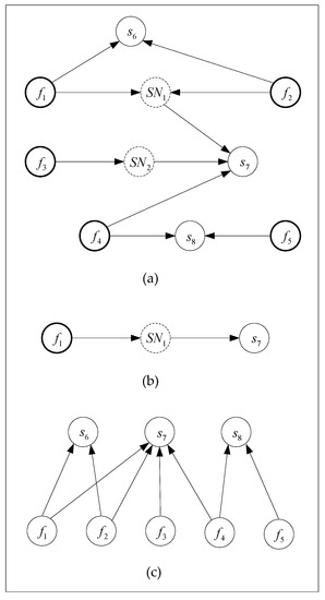
Figure 1.
Directed graph of an engineering system: (a) a directed graph; (b) a cause–effect graph of ; (c) a bipartite graph.
The structural representation of the system behavior using a directed graph helps to analyze the cause–effect relationships between faults and symptoms. A propagation path of the fault corresponding to the MSCC can be described via a cause–effect graph, which can be constructed by forward reasoning alongside the directed path corresponding to the fault. Each cause–effect graph has only one root node (an MSCC) in it, and a directed graph can be decomposed into plenty of cause–effect graphs, since there are usually many MSCCs in a directed graph. The symptoms of a fault in a cause–effect graph can be used to detect the presence of the fault. In the example above, a cause–effect graph regarding node is shown as Figure 1b. According to the cause–effect graph, the presence of fault can be observed by placing a sensor on node . It is not difficult to find that fault can also be detected via node if one constructs the other cause–effect graph of node .
The dependencies between faults and observable parameters can be described using a bipartite graph by removing the sequentially dependent faults and unobservable parameters in the cause–effect graphs. The parent and children nodes in the bipartite graph are instantiated as faults and sensors, respectively. A directed edge exists if a fault is perceived to be a direct cause of an abnormity . The bipartite graph of Figure 1a is shown as Figure 1c. The intermediate nodes denote the sequentially dependent faults, and hence unobservable parameters in the system can be removed from the graph. Nodes with only input edges denote the observable operating parameters in this system. It can be seen that the bipartite graph clearly shows the causal relationships between faults and symptoms from the complex directed graph.
According to the causal relationships represented in the bipartite graph, the fault signature matrix of the system can be consequently constructed. The fault signature matrix of the case in Figure 1 is shown as follows, which crosses a set of faults in rows and symptoms in columns. All faults in are observable since every row vector is not empty. Faults are non-isolatable because they have the same row vector. The example shows the procedure for constructing a fault signature matrix using a directed graph, which provides a basis to locate sensors in the system for desired fault isolatability.
4. Locating Sensors Using Population-Based Incremental Learning
According to the problem formulation in Section 2, the problem of sensor location based on fault isolatability criteria can be regarded as selecting a minimal set of sensors while keeping the capacity of fault isolation unchanged. Intuitively, the problem of sensor location can be dealt with by searching over all possible combinations of the sensors. But with tens of technical indicators available for condition monitoring of a complex engineering system, this strategy is thought to be intractable, as the quantity of sensor combinations will increase exponentially (known as a NP-hard problem). The heuristic method provides an effective way to solve this problem, and a well-known method among all kinds of heuristic methods is called the genetic algorithm (GA). The GA follows the principles of evolution and natural genetics and uses random steps to converge to a nonrandom optimal solution. This method has been successfully applied for solving combinatorial optimization problems in various research fields. However, the problem of “genetic drift” means the global optimum solution cannot be guaranteed. In this section, an estimation of distribution algorithm (EDA), called population-based incremental learning (PBIL), is used for this purpose. Different from the genetic algorithm (GA), PBIL regards population evolution as a process of learning [20,21]. The algorithm introduces a novel procedure of evolutionary computation using population learning while abandoning the conventional evolutionary operators, e.g., crossover and mutation [22,23]. Specifically, PBIL firstly constructs a probabilistic model to describe the individual distribution in the solution domain and then produces the next generation by statistically learning and sampling the probability distribution of the best individuals at each generation. The evolution in PBIL is essentially the population-level (population learning); therefore, PBIL has a better convergence rate compared with the GA [24], which is also the motivation of exploiting PBIL in the paper.
A binary encoded solutions string is firstly defined to describe the solution domain of the sensor location problem. For a complex engineering system with the fault signature matrix as , the solution domain for sensor location problem is denoted as , in which coding , which represents the sensor , is placed in the system, while , conversely. All the possible configurations of sensors are therefore represented as various combinations of 0s and 1s. In PBIL, each possible solution (a possible configuration of sensors) is called an individual and the binary code is called a gene. A number of individuals constitute a population. The quantity of individuals in a population is called the population size. The relationships among genes, individuals, and the population is described in Figure 2. A probability vector is used to guide to generation of individuals, where represents the probability of , while denotes the probability of . A gene with high probability tends to generate a 1 in the bit position instead of 0. The probability vector is firstly initialized as to randomly generate a population at the beginning of evolution and then is updated according to the probability distribution of the best individuals at the last generation. The update of the probability vector will increase the probability , corresponding to the bit position , where a 1 shows in the best individual. In this paper, the Hebb rule in machine learning was used to update the probability vector. The probability update rule can be written as:
where , denotes the probability vector of the -th and -th generation, respectively, and represents the learning rate, ; represents the -th best individual in the -th generation and denotes the quantity of best individuals.
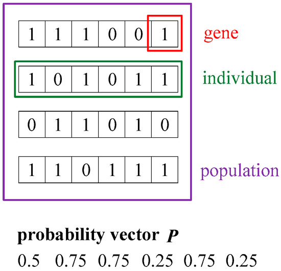
Figure 2.
Genetic representation of the solution domain.
The best individuals in a population was evaluated and then selected by calculating the fitness function. The individuals with a higher fitness function were expected to be better-adapted to the evolution, i.e., a more optimal solution for the sensor location problem. In this paper, the fitness function was defined as Equation (2).
The fitness function consists of two operators, i.e., and . In the operator , denotes the individual in the population; denotes the quantity of 1s in the bit positions of the individual , i.e., the quantity of selected sensors according to ; represents the quantity of bit position in an individual. The operator is constructed to make sure the individual with less quantities of selected sensors has a higher fitness value.
In the operator , denotes the conditional entropy of , given the subset of sensors , corresponding with , and represents the conditional entropy of , given the complete set of sensors , i.e., ; is a constant and is used to control the climbing speed with approaching to . The characteristic curve of operator is shown as Figure 3, in which the horizontal axis represents and the vertical axis denotes . The solid line represents the function with , , while the dash line denotes the configuration of , . The dot line has a while keeping the unchanged. It can be seen that the value of the penalty function will increase rapidly if is close to , while it will approach 0 if is much larger than . Therefore, the definition of the penalty function guarantees the best individual solution of sensor location, after which the evaluation does not decrease the capability to distinguish faults.
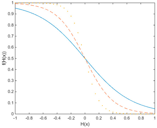
Figure 3.
The characteristic curve of the penalty function.
Parameters and were used to adjust the weight of operators and , according to the importance of each operator. Parameter was used to blend the sensor importance into the individual fitness value and normalizes the fitness function to a satisfying magnitude. The piecewise function is shown as Equation (3). The value will be 0 if all bit positions of are 0, i.e., , which minimizes the fitness of individual to 0 and therefore makes the individual be abandoned while evolving. The piecewise function is essentially a penalty function and was used to prevent a situation in which no sensor is selected in the process of solution searching.
Accordingly, factors and make the solution with less quantity of sensors and larger conditional entropy have higher fitness value, which is exactly the requirement of sensor location.
In order to speed up the evaluation, a heuristic function is defined in this paper to guide the selection of the best individual. The heuristic function was constructed according to the fact that sensors vary in the necessity to distinguish pairs of faults. To make it clear, the fault signature matrix of the system in Figure 1 was taken as an example. According to the fault signature matrix, sensor provides the only information to distinguish faults and . Therefore, sensor was the indispensable sensor for fault isolation of the system, whereas faults and varied in the reading of both and . Thus, sensors and can be substituted for each other in terms of distinguishing and . To describe the difference in necessity of sensors regarding fault isolation, the notion of attribute importance in information theory is introduced in this paper. The importance of a sensor is defined as follows.
Definition 3.
Given an engineering system, in whichand, letbe a subset of, e.g.,; the importance of a sensoris defined as.
The sensor with higher importance is more necessary for fault isolation. In the fitness function , factor was used to blend the sensor importance into the individual fitness value. If the sensor with is selected in the individual , , otherwise, .
According to the analysis above, the algorithm for sensor location using PBIL can be described as follows. In order to make the observability of each single fault be guaranteed, an auxiliary step was proposed by appending an extra sensor if there was a fault that went unobserved with the sensor configuration output by PBIL.
- Step 1.
- Calculate the conditional entropy of , given a complete set of sensors ;
- Step 2.
- Let , for each , if , then ;
- Step 3.
- If. , then output as the optimal solution; otherwise, go to Step 4;
- Step 4.
- Calculate the importance of each sensor , i.e., ;
- Step 5.
- Search the optimal sensor location solution using PBIL:
- Step 5.1.
- Generate a population based on the probability vector and let the bit position be 1 if the corresponding sensors are ;
- Step 5.2.
- Calculate the fitness value of each individual and sort the individuals according to the fitness values;
- Step 5.3.
- Select best individuals ; let be the sensor configuration suggested by and terminate the evaluation and output the optimal sensor location solution if , otherwise go to Step 5.4;
- Step 5.4.
- Update the probability vector using the Hebb rule according to the best individuals and turn to Step 5.1.
- Step 6.
- For a fault signature matrix consisting of and , if , then , , where is an element in .
5. Case Study
5.1. Sensor Location of a Diesel Engine
The first case comes from Yan and Huang [25]. The diesel engine, as the most widely used power machinery, plays an important role in all fields of social economy, e.g., ship power, railway transportation, and oil drilling. The increasing demand for engine reliability and emission motivates the research on condition monitoring and health management. The common faults and observable parameters of a diesel engine are listed in Table 1 and Table 2, respectively.

Table 1.
Common faults of a diesel engine.
Table 2.
The observable parameters of a diesel engine.
Many studies have been devoted to the failure mechanism and fault feature extraction of diesel engines. Currently, researchers have been detecting and identifying the common faults of diesel engines using information output from different types of sensors. According to their research, the fault signature matrix of diesel engines, regarding faults and sensors shown in Table 1 and Table 2, can be presented as follows.
The algorithm proposed in Section 4 is used to locate the minimum quantifier of sensors for fault isolation of a diesel engine. The parameters in the algorithm are set as: population size , learning rate , and best individuals to update the probability vector ; parameter in operator is , the weights of operators and are and , respectively. If the sensor with is selected, , otherwise . The maximum evolution generation . Table 3 shows the selected optimal configuration of sensors using the proposed approach.
Table 3.
Comparisons of the proposed approach with the approach in Reference [25].
Using the PBIL-based approach, is derived as the quantity-optimum set of sensors for the purpose of fault isolation. Compared with the original sensor network, the sensor configuration solution derived using the PBIL-based approach reduces the required number of sensors from 12 to 7, which remarkably reduced the difficulty to obtain complete information of engine behavior for the purpose of fault isolation. The validity of the sensor location solution can be verified according to the fault signature matrix of a diesel engine. It can be seen that the element value in the fault signature matrix, corresponding to , can vary from row to row, which means that there is always a sensor that can be used to distinguish pairs of faults of a diesel engine. For example, misfire will lead to the abnormal reading of sensor , as well as , while the cylinder score can be sensed via , , and . Therefore, the faults and can be distinguished by sensors and .
As a comparison, the result from the sensor network proposed by Yan and Huang [25] is also presented in Table 3. This approach designs the sensor network based on observability criteria. Therefore, sensors and are calculated as the indispensable one. From the fault signature matrix, it can be seen that faults can be detected via sensor , since the corresponding element value is 1 in the matrix. Similarly, faults can be detected via sensor . The set of sensors is sufficient to detect the presence of all faults; however, it cannot identify the root cause of an abnormity. For example, both faults and can lead to the abnormal reading of sensors and , which means that these two faults cannot be distinguished by sensors and . The comparison with the sensor location approach in [25] shows that the PBIL-based approach can minimize the quantity of sensors while keeping the ability of fault isolation unchanged.
5.2. Sensor Location in a FCCU
Raghuraj proposes a classical sensor location approach based on isolatability criteria, and the approach is illustrated on a fluid catalytic cracking unit (FCCU) [8]. In this section, the proposed approach is also demonstrated using the FCCU to verify the validity.
The common faults and sensors often used for condition monitoring of a FCCU are shown in Table 4 and Table 5, respectively. According to the fault analysis in Reference [8], the fault behavior of a FCCU can be described using a directed graph, as shown in Figure 4.
Table 4.
Common faults of a fluid catalytic cracking unit (FCCU).
Table 5.
The observable parameters of a FCCU.
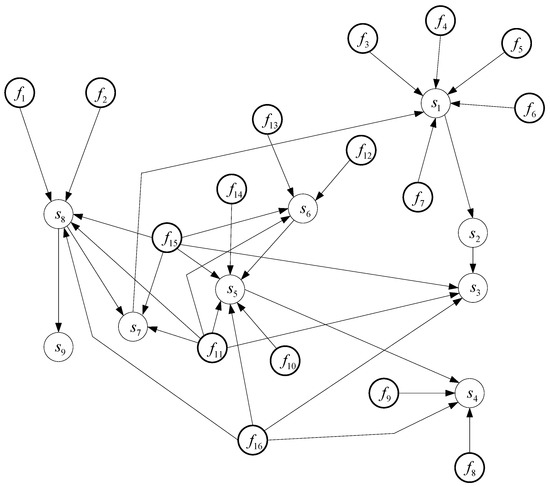
Figure 4.
The directed graph of a FCCU.
According to the directed graph presented in Figure 4, the fault signature matrix of a FCCU can be presented as follows.
It may be noted that faults , , , , , and cannot be distinguished from each other, even given the complete set of sensors. The PBIL-based algorithm is used to select a quantity-optimum set of sensors for the derived fault isolation. The optimal sensor location solution according to the PBIL-based algorithm is shown as column 3 in Table 6. The sensor network designed using the graphical method presented in Reference [8] is listed as column 2 in Table 6 as a comparison.
Table 6.
Comparisons of the proposed approach with the approach in Reference [8].
Using the PBIL-based approach, sensors are necessary for the fault isolation of a FCCU. This may be not consistent with the sensor location solution derived by the graphical method in Reference [8], which shows sensors are the indispensable sensors for fault isolation. However, according to the fault signature matrix, it can be found that both and can distinguish the multiple faults of a FCCU to the maximal extent. Therefore, there are multiple options of locating a quantity-optimum set of sensors for fault isolation. Using the PBIL-based approach, only five sensors are needed for the condition monitoring and fault isolation of a FCCU by eliminating four redundant sensors, which simplifies the sensor network for condition monitoring and fault isolation.
6. Conclusions
In this paper, a PBIL-based sensor location approach is proposed for the purpose of fault isolation. The approach takes use of the fault signature matrix to describe the multidimensional causal relationships of faults and symptoms. The problem of sensor location is then formulated as an optimization problem and handled using the PBIL algorithm. The sensor importance is defined using information theory as a heuristic function to guide the process of sensor location. The proposed approach is illustrated via two classical cases. The results show that the PBIL-based approach reduces the quantity of sensors from 12 to 7 in the diesel engine case and from 9 to 5 in the fluid catalytic cracking unit case, which reduces the difficulty of applying condition monitoring and fault isolation in practice.
Author Contributions
Conceptualization, J.W., Z.W., and X.M.; methodology, J.W. and G.F.; software, J.W. and C.Z.; validation, J.W. and G.F.; formal analysis, C.Z.; investigation, J.W.; resources, X.M. and G.F.; data curation, C.Z.; writing—original draft preparation, J.W.; writing—review and editing, J.W., X.M., and G.F.; visualization, C.Z.; supervision, Z.W. and X.M.; project administration, Z.W.; funding acquisition, Z.W. All authors have read and agreed to the published version of the manuscript.
Funding
This research was funded by The National Natural Science Fund of China, grant number 51305089, and Natural Science Foundation of Heilongjiang Province of China, grant number E2016018.
Conflicts of Interest
The authors declare no conflict of interest.
References
- Liu, R.; Yang, B.; Zio, E.; Chen, X. Artificial intelligence for fault diagnosis of rotating machinery: A review. Mech. Syst. Signal Process. 2018, 108, 33–47. [Google Scholar] [CrossRef]
- Hwang, I.; Kim, S.; Kim, Y.; Seah, C. A survey of fault detection, isolation, and reconfiguration methods. IEEE Trans. Control Syst. Technol. 2010, 18, 636–653. [Google Scholar] [CrossRef]
- Wang, H.; Wang, H.; Jiang, G.; Li, J.; Wang, Y. Early fault detection of wind turbines based on operational condition clustering and optimized deep belief network modeling. Energies 2019, 12, 984. [Google Scholar] [CrossRef]
- Janssens, O.; Slavkovikj, V.; Vervisch, B.; Stockman, K.; Loccufier, M.; Steven, V.; Walle, R.; Hoecke, S. Convolutional neural network based fault detection for rotating machinery. J. Sound Vib. 2016, 377, 331–345. [Google Scholar] [CrossRef]
- Duan, R.; Lin, Y.; Feng, T. Optimal sensor placement based on system reliability criterion under epistemic uncertainty. IEEE Access 2018, 6, 57061–57072. [Google Scholar] [CrossRef]
- Bhushan, M.; Rengaswamy, R. Comprehensive design of a sensor network for chemical plants based on various diagnosability and reliability criteria. 1. framework. Ind. Eng. Chem. Res. 2002, 41, 1826–1839. [Google Scholar] [CrossRef]
- Bhushan, M.; Rengaswamy, R. Comprehensive design of a sensor network for chemical plants based on various diagnosability and reliability criteria. 2. applications. Ind. Eng. Chem. Res. 2002, 41, 1840–1860. [Google Scholar] [CrossRef]
- Raghuraj, R.; Bhushan, M.; Rengaswamy, R. Locating sensors in complex chemical plants based on fault diagnostic observability criteria. AIChE J. 1999, 45, 310–322. [Google Scholar] [CrossRef]
- Sahoo, S.; Yin, X.; Liu, J. Optimal sensor placement for agro-hydrological systems. AIChE J. 2019, 65, 1–18. [Google Scholar] [CrossRef]
- Oskouei, F.; Pourgol-Mohammad, M. Optimal sensor placement for efficient fault diagnosis in condition monitoring process: A case study on steam turbine monitoring. In Current Trends in Reliability, Availability, Maintainability and Safety; Springer: Berlin/Heidelberg, Germany, 2016; pp. 83–97. [Google Scholar]
- Oskouei, F.; Pourgol-Mohammad, M. Fault diagnosis improvement using dynamic fault model in optimal sensor placement: A case study of steam turbine. Qual. Rel. Eng. Int. 2017, 33, 531–541. [Google Scholar] [CrossRef]
- Oskouei, F.; Pourgol-Mohammad, M. Sensor placement determination in system health monitoring process based on dual information risk and uncertainty criteria. Proc. Inst. Mech. Eng. O J. Risk Reliab. 2017, 232, 65–81. [Google Scholar]
- Perelman, L.; Abbas, W.; Koutsoukos, X.; Amin, S. Sensor placement for fault location identification in water networks: A minimum test cover approach. Automatica 2016, 72, 166–176. [Google Scholar] [CrossRef]
- Chen, C.; Chen, L.; Ding, J.; Wu, Y. The effectivity analysis of adding sensors for improving model based fault isolability properties. J. Process Control 2018, 70, 123–132. [Google Scholar] [CrossRef]
- Travé-Massuyès, L.; Escobet, T.; Olive, X. Diagnosability analysis based on component-supported analytical redundancy relations. IEEE Trans. Syst. Man Cybern. Syst. 2006, 36, 1146–1160. [Google Scholar] [CrossRef]
- Chi, G.; Wang, D. Sensor placement for fault isolability based on bond graphs. IEEE Trans. Autom. Control 2015, 60, 3041–3046. [Google Scholar] [CrossRef]
- Rosich, A.; Frisk, E.; Åslund, J.; Sarrate, R.; Nejjari, F. Fault diagnosis based on causal computations. IEEE Trans. Syst. Man Cybern. Syst. 2012, 42, 371–381. [Google Scholar] [CrossRef]
- Chi, G.; Wang, D.; Le, T.; Yu, M.; Luo, M. Sensor placement for fault isolability using low complexity dynamic programming. IEEE Trans. Autom. Sci. Eng. 2015, 12, 1080–1091. [Google Scholar] [CrossRef]
- Miao, D.; Wang, J. An information representation of the concepts and operations in rough set theory. J. Softw. 1999, 10, 113–116. [Google Scholar]
- Sleesongsom, S.; Bureerat, S. Morphing wing structural optimization using opposite-based population-based incremental learning and multigrid ground elements. Math. Probl. Eng. 2015, 2015, 730626. [Google Scholar] [CrossRef]
- Grisales-Noreña, L.; Montoya, D.; Ramos-Paja, C. Optimal sizing and location of distributed generators based on PBIL and PSO techniques. Energies 2018, 11, 1018. [Google Scholar] [CrossRef]
- Ho, S.; Yang, J.; Yang, S.; Bai, Y. A real coded vector population-based incremental learning algorithm for multi-objective optimizations of electromagnetic devices. IEEE Trans. Magn. 2018, 54, 700304. [Google Scholar] [CrossRef]
- Xue, X.; Chen, J. Optimizing ontology alignment through hybrid population-based incremental learning algorithm. Memet. Comput. 2019, 11, 209–217. [Google Scholar] [CrossRef]
- Chen, M.; Chang, P.; Wu, J. A population-based incremental learning approach with artificial immune system for network intrusion detection. Eng. Appl. Artif. Intell. 2016, 51, 171–181. [Google Scholar] [CrossRef]
- Yan, P.; Huang, X.; Lian, G.; Zhang, Y. Research on multi-class sensor placement optimization method for fault diagnosis of mechanical power and transmission system based on fault-sensor dependence matrix. Comput. Meas. Control 2012, 20, 1753–1756. [Google Scholar]


© 2020 by the authors. Licensee MDPI, Basel, Switzerland. This article is an open access article distributed under the terms and conditions of the Creative Commons Attribution (CC BY) license (http://creativecommons.org/licenses/by/4.0/).