Abstract
The area-proportional baseline method generates phase fraction–temperature curves from heat capacity data of phase change materials. The curves describe the continuous conversion from solid to liquid over an extended temperature range. They are consistent with the apparent heat capacity and enthalpy modeling approach for the numerical solution of heat transfer problems. However, the curves are non-smooth, discrete signals. They are affected by noise in the heat capacity data and should not be used as input to continuous simulation models. This contribution proposes an alternative method based on spline approximation for the generation of consistent and smooth phase fraction–temperature, apparent heat capacity–temperature and enthalpy–temperature curves. Applications are presented for two commercial paraffins from Rubitherm GmbH considering heat capacity data from Differential Scanning Calorimetry and 3-layer-calorimetry. Apparent heat capacity models are validated for melting experiments using a compact heat exchanger. The best fitting models and the most efficient numerical solutions are obtained for heat capacity data from 3-layer-calorimetry using the proposed spline approximation method. Because of these promising results, the method is applied to melting data of all 44 Rubitherm paraffins. The computer code of the corresponding phase transition models is provided in the Supplementary Information.
1. Introduction
Paraffin waxes are interesting candidates as phase change materials (PCM). They are commercially available for a wide range of melting temperatures, relatively low in cost and have a good thermal reliability [1,2]. However, technical-grade materials and mixtures mostly show a non-isothermal phase change which takes place over an extended temperature range. Moreover, paraffin systems sometimes show two different phase transitions in the interesting temperature operating range. This phenomenon is not unusual and can be explained by a low temperature solid–solid transition and a high temperature solid–liquid transition [3,4,5,6,7,8]. Another possible explanation could be the different chain lengths in mixtures of different compounds [8]. Suitable models for a reasonably accurate description of this complex phase transition behavior are needed to assess the performance of latent heat thermal energy storage systems using paraffins as PCM.
The most popular approaches for the mathematical modeling of phase change problems in PCM are the enthalpy method, the apparent (or effective) heat capacity method, and the source based method [9]. Following these approaches, a mushy transition zone between the two (solid and liquid) phases is considered. In this zone, a single enthalpy–temperature, apparent heat capacity–temperature, or a heat flux-temperature curve is applied. The numerical solution takes place on a fixed-space grid [9].
The definition of the local liquid fraction is a key feature for the application of the apparent heat capacity and source-based methods [10]. Within the phase transition temperature range, the structure of the PCM is approximated by the solid and the liquid phase [10]. Accordingly, the progress of the phase change is determined by the liquid fraction and the apparent (or effective) specific heat capacity is modeled by contributions from the two phases and the phase transition enthalpy [11,12]. While, for the energy balance equation, the mass liquid fraction is used, for the momentum equation, the volumetric liquid fraction (or porosity) is used [13,14,15].
The local liquid fraction depends on the phenomena occurring during the PCM’s phase transitions during heating (melting) and cooling (solidification). Their complexity is usually determined by the nature of the solidification process. e.g., as pointed out by Voller et al. [10], if the kinetics of the transformation are such that under-cooling is significant, the local liquid fraction might depend on temperature, cooling rate, nucleation rate, and solidification speed. In addition, in multi-component materials, solutal transport (macro-segregation) will also influence the local liquid fraction (field) [10].
However, for many systems, it can be reasonably assumed that the liquid fraction is a function of temperature alone [9]. Caggiano et al. [16] provide a recent review of temperature-dependent apparent (or effective) heat capacity models in the framework of fixed-grid methods. It is noted that not all of the reviewed models explicitly consider the liquid fraction as a system state. However, because of the direct relation between the liquid fraction and the heat capacity, [11,12,17] these models fall into the same category. The same applies for models defined by enthalpy–temperature curves, see e.g., [18]. The heat capacity models in Caggiano et al. [16] use smooth and non-smooth transition functions, including interpolation functions using tabulated data from differential scanning calorimetry (DSC) [19].
The most straightforward way to model phase fraction–temperature curves is to define a linear function between the liquidus and solidus temperatures, see e.g., [15]. This approach can also be used for PCM with an isothermal phase change introducing a small artificial temperature region, see [10] and FLUENT Manual [20]. Enthalpy–temperature and heat capacity–temperature curves are also often designed to match the results of heat capacity data, e.g., generated by DSC or 3-layer-calorimetry. These curves then correspond to data recorded during complete melting, complete solidification, or to intermediate curves between both, see e.g., [18,21,22,23,24,25,26,27]. They are usually modeled e.g., by piecewise linear functions [28], probability distribution functions [12,17], cubic spline interpolating polynoms [29]. As an alternative, Franquet et al. [30] propose to solve an inverse identification problem to identify parameters of a thermodynamical model of the sample’s heat capacity. In the same way, DSC heat capacity data given as heat flow-temperature curve can be considered for the source-based methods [31,32,33,34].
It is noted that all aforementioned contributions implement static phase transition models which are independent of the applied heating or cooling rate [12]. However, heat capacity data, such as generated by DSC, is highly sensitive to the applied heating and cooling rates and the sample mass [23,35]. PCM phase transition behavior is also scale dependent [35,36]. A direct strategy to account for this is the consideration of different phase transition models depending on the direction and rates of temperature changes in the studied application, e.g., [12,17,18,37]. Moreover, various extensions of the numerical methods have been proposed in order to account for (subcooling) supercooling phenomena, e.g., combining enthalpy curves for (super-)cooling with kinetic models for crystal growth [38,39], using punctionally negative apparent heat capacities to mimic the temperature growth in a recrystalling material [40], and considering an internal heat source in the PCM which is activated at a defined (supercooled) temperature [41].
Phase fraction–temperature curves can be generated by baseline construction [42,43]. This method is usually applied for the analysis of thermal events in DSC heat capacity data, where the events are characterized by a peak in the recorded signal in a specific temperature range. These events can be e.g., thermoplastic melting or crystallization, or thermoset curing [44]. DSC heat capacity data represents overall (apparent) heat capacities. The net effect of thermal events is obtained after substraction of the baseline from the recorded overall heat capacity [42,44,45]. Different alternative approaches exist for baseline construction: formal methods, e.g., using straight lines or sigmoidal curves, and methods with a physico-chemical assumption on the change of the heat capacity during transition, e.g., using exponential curves [42,43]. The (tangential) area-proportional baseline method uses an iterative numerical integration algorithm to evaluate decomposition reactions and generate conversion-temperature curves [46]. The application to PCM heat capacity data for identification of baseline and phase fraction curves was demonstrated e.g., by Diaconu et al. [47].
In this contribution, an alternative method for identification of phase fraction–temperature curves from heat capacity data of solid–liquid PCM is proposed. The curves are indirectly recovered from the shape of the measured (overall) peak signals. The proposed method uses the same assumptions as the area-proportional baseline method. However, while the area-proportional baseline method calculates discrete signals, the proposed method generates smooth functions:
- The proposed method has the following advantages over the above described methods for the identification of enthalpy–temperature, apparent heat capacity–temperature, or heat flux–temperature curves: It generates phase fraction–temperature curves represented by smooth functions which accurately adapt to the shape of the measured peak signals, i.e., no prior assumptions need to be taken on the curve shape. They predict the degree of conversion of the phase transition process, and are consistent with the two-phase apparent heat capacity modeling approach. Thus, they are especially suited for the efficient numerical solution of heat transfer problems in solid–liquid PCM.
- In contrast to most of the previous works on the determination of PCM thermophysical properties, this contribution includes a critically evaluation of the predictive performance of the identified phase transition functions when used for simulation of a thermal energy storage with PCM. Results are presented for heat capacity data of RT35HC and RT44HC from Rubitherm GmbH (Berlin, Germany) generated by DSC and 3-layer-calorimetry. The derived functions are validated for melting experiments in a compact extended surface aluminium heat exchanger (HEX). The models identified from DSC data show a poor fitting. However, good results are obtained for data from 3-layer-calorimetry.
- Because of these promising results, the proposed method is applied to melting data from 3-layer-calorimetry of all 44 available Rubitherm RT paraffins. The computer code of the derived phase fraction–temperature, apparent heat capacity–temperature and enthalpy–temperature curves is provided in the supplementary information.
The remainder of this paper is structured as follows. Section 2 introduces the methods to produce heat capacity data. The two-phase apparent heat capacity model and the area-proportional baseline method are reviewed. The latter uses numerical integration of heat capacity data and generates discrete signals. In Section 3, an alternative method is proposed which is based on spline interpolation and generates smooth functions. In Section 4, both methods are applied to heat capacity data of two commercial PCM for which data are available from DSC and 3-layer calorimetry. The identified curves are used for the numerical modeling of heat transfer in a compact HEX filled with PCM. Details on the predictive performance of the models and numerical aspects of their implementation are given. Finally, Section 5 gives a discussion and conclusions.
2. Materials and (Established) Methods
2.1. Specific Heat Capacity Measurements
Heat capacity data were generated by heat flow differential scanning calorimetry (hf-DSC) using a NETZSCH DSC 404C (Erich Netzsch GmbH & Co. Holding KG, Selb, Germany) and following the procedures described in the IEA SHC TASK 42/ECES Task 29 [48]. The sample mass of RT35HC was 11.99 mg and of RT44HC was 11.73 mg. Aluminum crucibles (25 L) with pierced lids were used, and a helium atmosphere was applied (gas flow 50 mL/min). Data was collected at a constant temperature rate of 0.1 K/min after preheating of the samples to the maximum set temperature. This relatively low rate was chosen in order to reduce the thermal gradients in the sample and the DSC apparatus. Accordingly, the smearing of the recorded peak signals was also reduced and almost uniform sample temperature and equilibrium conditions can be assumed. The heat capacity data are stored as “continuous” data, sampled on small intervals of 0.002 K. For the determination of , the area proportional baseline method was applied and the peak area was numerically integrated. The following values were found: 224.9 J/g for RT35HC and 229.8 J/g for RT44HC. For validation, data were also collected at 1.0 and 10.0 K/min. The maximum relative difference between the three results for is 0.51% (RT35HC) and 0.33% (RT44HC), which highlights the accuracy of the DSC measurements. To obtain accurate results for the specific heat capacities outside the phase transition temperature range, experiments were conducted at an increased temperature rate of 20 K/min using three samples with masses ranging from 20.30 to 21.33 mg. It is noted that in this contribution solid and liquid heat capacities are assumed constant. The following values are used 2.6 J/(g·K) (solid) and 2.8 J/(g·K) (liquid). Similar values are found in literature for commercial paraffin waxes, see e.g., [6,8].
In addition, heat capacity data were considered as given in the PCM datasheet provided by Rubitherm GmbH (Berlin, Germany). These data were generated by 3-layer-calorimetry [49,50]. In addition, 3-layer-calorimetry measures the heat flux in/out of the sample via a calibrated resistance. In contrast to hf-DSC, rather large sample sizes are used in order to get more representative results for inhomogeneous systems, see Vidi et al. [51] for details. Moreover, the temperature rate and heat fluxes are not constant during the measurement procedure. They depend on the material properties of the sample. The realized heating and cooling rates are well below 0.1 K/min [52]. According to recommendations by Mehling and Cabeza [53], the heat capacity data collected by 3-layer-calorimetry are given as stored heat in 1.0 K intervals.
2.2. The Two-Phase Rate-Independent Apparent Heat Capacity Model
For mixtures and technical-grade PCMs, the solid–liquid phase change occurs within a specific temperature range. Within this range, it is assumed that the structure of the PCM can be approximated by two coexisting phases, a solid and a liquid phase [11]. Accordingly, phase transitions can be modeled by one characteristic parameter:
where is the (liquid mass) phase fraction, and and are the masses of solid and liquid phase, respectively. It is assumed that the phase fraction is a function of temperature alone: . It is further assumed that the phase transition function monotonously increases with rising temperature and that it realizes a smooth transition from (completely solid phase) to (completely liquid phase).
Following the two-phase modeling approach, the apparent (or effective) heat capacity is modeled by a linear superposition of terms for solid () and liquid () heat capacity as well as the phase transition enthalpy () [11]:
where is the temperature-dependent phase transition function and is its derivative. Because the function depends on temperature alone, Equation (2) is a rate-independent model which assumes that solid and liquid phase are always in equilibrium.
2.3. Area-Proportional Baseline Method for Identification of Phase Fractions as Discrete Signals
Following the two-phase apparent heat capacity modeling approach the data from the measurement procedures in Section 2.1 represent apparent specific heat capacities, as defined in Equation (2). Within the phase transition temperature range, the contributions from the solid and liquid heat capacities (in the following referred to as baseline) and the phase transition enthalpy are not determined individually.
In the area-proportional baseline method, the heat capacity of the system (the baseline) is assumed to change continuously from the level at the start of the transition to the level at the end of the transition. This change is assumed to be proportional to the degree of conversion [42,44]. For solid–liquid transitions, the degree of conversion is defined by the (liquid mass) phase fraction , see Equation (1). (Note that in DSC analysis is often also referred to as degree of conversion or phase change progress parameter, see e.g., [42,44].) The area-proportional baseline method computes the gradual change in during the transition, i.e., from zero to unity. The result is a phase fraction–temperature curve. This curve defines the course of the heat capacity change in the region of the peak (the baseline).
It is assumed that the DSC data are corrected for the instrumental baseline and internal delays and is given as function of temperature [44]. The following definitions are used for the baseline and the phase fraction [46]:
where the variables a and b denote the limits of the phase transition temperature range. In the “tangential” area-proportional baseline method, the heat capacities and are modeled by linear functions of the temperature:
The linear functions (and their coefficients ) are determined by tangents at the left and right end of the DSC curve (after cutting the part from a to b) [46]. The baseline construction is performed by numerical integration of Equation (3b) and inserting the result in Equation (3a). To this end, , , and are considered as discrete signals sampled at temperatures with such that . As is a function of which is a function of the unknown , must be solved iteratively. The iterations are initialized approximating by a linear interpolation between and . Based on this first approximation, is updated. The procedure is repeated until a suitable convergence criterion is fulfilled (see [44,46] for details).
It is interesting to note that the baseline in Equation (3a) is defined (in the same way as in Equation (2) by contributions of terms for liquid () and solid () heat capacities. Inserting Equation (3a) in Equation (2) yields:
and after integrating from a to T the same expression as in Equation (3b) is obtained:
It can be concluded that the definition of in Equation (3b) is consistent with the model for the apparent specific heat capacity in Equation (2). Thus, the results of the numerical integration method (i.e., the discrete signals and ) are also consistent with the two-phase model in Equation (2).
3. Proposed Method for Identification of Smooth Phase Transition Functions
An alternative method based on piecewise spline interpolation is presented which generates continuous phase transition functions from heat capacity data. The method is also consistent with the model for in Equation (2). As in Section 2.3, it is assumed that there is a clear start and end of the phase transition defining the phase transition temperature range, and that the (single phase) solid and liquid specific heat capacities are constant. Moreover, conditions are formulated such that the interpolation method yields a three times continuously differentiable ( smooth) transition function. Accordingly, using the transition function and its derivative with Equation (2), the model for is then twice continuously differentiable ( smooth).
The method is derived and exemplarily illustrated for RT35HC heat capacity data as provided by Rubitherm GmbH. Note that, while the data are given as partial enthalpies , these values are (approximately) taken here as apparent specific heat capacities: . This is reasonable as the specific partial enthalpies are defined for relatively small temperature intervals of K.
3.1. Identification of Solid and Liquid Heat Capacities and the Phase Transition Temperature Range
The heat capacity data are shown in Figure 1 and is defined over a temperature interval , where a and b are the start and end of the phase transition temperature range, respectively. The available data do not seem reliable for determining a and b as well as and (outside the phase transition temperature range). Therefore, these quantities were chosen after best knowledge, see Section 4.1 for a discussion of these issues in the context of DSC measurements. The values of the transformed heat capacity data are also shown in Figure 1.
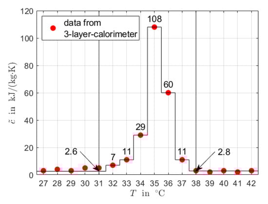
Figure 1.
RT35HC heat capacity data for heating given as partial enthalpies. The original data are transformed to apparent specific heat capacities. Moreover, the start and end of the phase transition temperature range and constant solid and liquid properties and , respectively, are defined.
3.2. The Interpolation Model
Phase transitions are modeled using piecewise spline interpolating polynoms :
where each interpolation interval is divided by the grid points
with such that . For the example in Figure 1 with C and C, . For each of the intervals the splines are defined as:
where
is the polynomial order and
are the unknown polynomial coefficients. The splines are defined by the following conditions:
- interpolation conditions:
It is noted that, in Equation (9), it is assumed that is directly measured at points with with the corresponding values . As discussed before, this is not true. A proper transformation of Equation (9) is proposed in the next section which replaces the values by caloric measurements.
- conditions for the differentiability at the inner grid points:
- 6 boundary conditions at the start () and end () of the transition region:
For this variable order spline interpolation, the conditions in Equations (9a) to (9c) constitute a linear equation system whose solutions are the unknown coefficients .
3.3. Identification of Polynomial Coefficients
In the previous section, it was assumed that is directly measured, see Equation (9a). In this section, this assumption is dropped and the measured heat capacity data are considered. These data are the values , taken at points with as shown in Figure 1. Equations (2) and (7) yield:
For constant thermo-physical properties , the apparent specific heat capacity is a linear function of the splines and their first derivatives :
The conditions in Equation (9a) can now be replaced by:
- interpolation conditions:
The conditions in Equations (9b), (9c) and (12) constitute a linear equation system whose solutions are the unknown coefficients . The values of , are directly defined by the corresponding measurements taken at and :
The remaining unknown variable is the phase transition enthalpy . Figure 2a shows results for the solution of the linear system defined by Equations (9b), (9c), (12) and (13) for different values of .
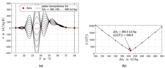
Figure 2.
Piecewise spline interpolation for the data given in Figure 1. (a) Identified interpolating polynoms for different values of . (b) Minimization of the arc length of the interpolated apparent specific heat capacity (problem Equation (14)). Each value of marked by a black dot corresponds to one polynom in (a).
From the point of view of available data, the most reasonable interpolation is a curve for with a minimum arc length . Thus, can be calculated by minimization of on the interval , i.e., between the two points and . The minimization problem reads:
where the length of each line segment is approximated by
and with being the sum of line segments, and with .
4. Results
4.1. Identification of Discrete Phase Fraction Temperature Signals
Results for the application of the area-proportional baseline method in Section 2.3 to heat capacity data of RT35HC and RT44HC are shown in Figure 4. The data are generated by hf-DSC. For RT35HC, one highly asymmetric peak is found in . For RT44HC, two peaks are found, one major highly asymmetric peak and a rather symmetric minor peak located at lower temperatures. The existence of two peaks is not unusual for commercial technical grade paraffin waxes and mixtures. This phenomenon can either be explained by multi-step phase transition, where transition at lower temperatures is the solid–solid phase transition and the transition at higher temperatures is solid–liquid transition, or it could be the result of a mixture of different compounds, having different chain lengths [8].
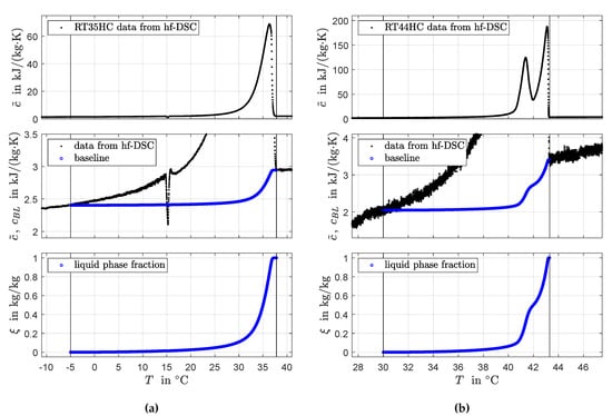
Figure 4.
Area-proportional baseline method applied to heat capacity data from hf-DSC. (a) RT35HC data recorded at 1 K/min. (b) RT44HC data recorded at 0.1 K/min. The slopes of and at the start and end of the phase transition temperature range are neglected. Baseline and phase fractions are constructed as discrete signals by numerical integration. The sudden jump in the DSC signal on the left around 15 °C is caused by a momentary deviation of the temperature controller from the programmed heating rate.
In order to reduce the influence of thermal gradients in the sample, the data are recorded at low heating rates. Usually, heating rates well below 1 K/min are recommended [8]. However, at lower heating rates, the signal-to-noise ratio decreases considerably and the influence of noise increases; compare the results recorded at 1 K/min and 0.1 K/min in Figure 4a,b, respectively.
In the second subfigures from above in Figure 4, it can be seen that the apparent heat capacity shows a smooth transition from the initial baseline to the ascending slope of the peak instead of a discontinuity. Therefore, the exact determination of the peak start (the limit a of the integral in Equation (3b) is difficult. This issue is not unusual, see e.g., Hemminger and Sarge [42]. Consequently, the slope of the baseline at the peak start is also difficult to estimate. For these reasons, in the same way as e.g., in Diaconu et al. [47], the temperature dependencies of and in Equation (3a) are dropped and constant values are used instead. Accordingly, as originally proposed by Bandara [44]. The constructed phase fraction–temperature curves are shown in the third subfigures from above. It can be seen for RT35HC and RT44HC that, although a relatively wide phase transition temperature range is selected, the significant changes in the phase fraction take place in a much smaller temperature range where the peak is located in .
Figure 5 shows results for data generated by 3-layer-calorimetry. Because the heat capacity data are given on a coarse grid, the resolution of the generated discrete signals is low. Note that there is no clear indication for two peaks in the data for RT44HC. Moreover, similarly as for the data generated by hf-DSC, there is no clear start and end of the phase transition temperature range and simplifying assumption need to be taken for the values for and .
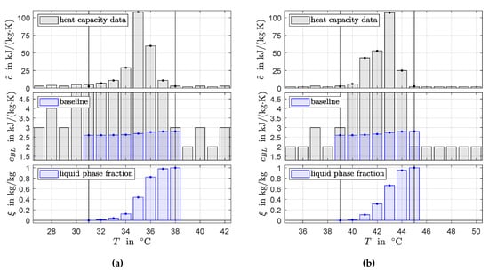
Figure 5.
Area-proportional baseline method applied to heat capacity data from 3-layer-calorimetry for RT35HC (a) and RT44HC (b). The values of and at the start and end of the phase transition temperature range were corrected. Baseline and phase fractions are constructed as discrete signals by numerical integration.
4.2. Identification of Smooth Phase Transition Functions
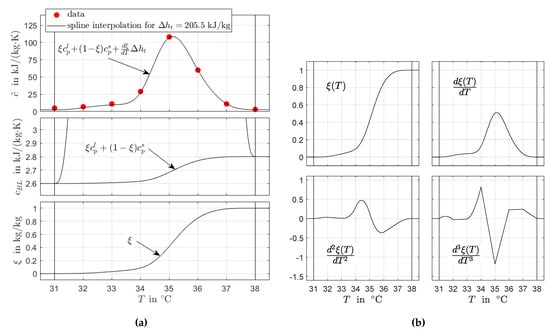
Figure 6 shows results for the application of the spline interpolation method in Section 3. Note that, for both PCM, the data from hf-DSC were recorded at 0.1 K/min (contrary to the data in Figure 4). Table 1 compares these results with results from the the area-proportional baseline method in Section 2.3.
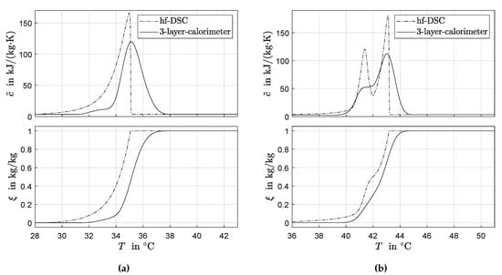
Figure 6.
Identified consistent phase transition functions and corresponding apparent heat capacity curves using spline interpolation for RT35HC (a) and RT44HC (b).

Table 1.
Results from spline interpolation (SI) and from area-proportional baseline (numerical integration, NI) method.
For the hf-DSC data recorded at 0.1 K/min, the spline interpolation uses a non-uniform grid with 50 (in case of RT35HC) and 65 (in case of RT44HC) points and a varying between 0.05 K and 5 K. The relatively dense grid is chosen to capture the steep slopes around the peak maxima in the recorded data. Because of the relatively low heating rate and corresponding low signal-to-noise ratio, there is a clear influence of noise in the DSC data. The influence of noise can be seen in the second subfigure in Figure 4b and is especially pronounced for low values of the heat capacity data. The spline interpolation uses an adaptive grid with relatively large steps in this temperature range to increase the robustness against noise. It is noted that the baseline (and also the phase transition-temperature curve ) as computed by the area-proportional baseline method shows a certain robustness against noise in the DSC peak signal. This is to be expected as (and also ) corresponds to the scaled cumulative integral of the DSC peak. The integrand cancels the noise. The same is observed for the value of which is obtained by peak integration. However, using the discrete signal to calculate the influence of noise does not vanish. The reason is that the peak in depends on the derivative of , see Equation (2).
The data collected by 3-layer-calorimetry are given on a coarse grid with eight (in case of RT35HC) and seven (in case of RT44HC) values in the phase transition temperature range. The same grids are used for both numerical integration and spline interpolation. Consequently, both methods yield exactly the same values for the apparent specific heat capacity at the sampling points. From the differences between values for and the maximum differences between values for reported in Table 1, it can be seen that both methods yield almost identical results.
4.3. Experimental Analysis of Heat Transfer with Phase Change
The applicability of identified phase fraction temperature curves is tested by comparison of predicted and measured PCM temperatures in a small compact extended surface HEX filled with RT35HC and RT44HC. The experimental setup is shown in Section 4.3. The HEX (Figure 7) is made from aluminium by AKG Verwaltungsgesellschaft mbH (Hofgeismar, Germany). The internals consist of two parallel liquid passages and three air passages. The liquid passages are extruded pipes, each 1.8 mm thick and 45 mm long. The air passages are 10.4 mm thick and enclose the two liquid passages, one air passage is located between the two liquid passages, see Figure 7 below.
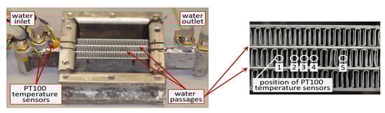
Figure 7.
Experimental setup for the characterization of the PCM phase transition behavior in a compact extended surface HEX. The air passages are filled with PCM. Water flows through the two liquid passages. Five PT100 temperature sensors are installed in the middle between the two liquid passages to measure the temperatures in the PCM passage. Two PT100 are installed at the outer surface of the two liquid passages.
The air passage use offset strip fins (width 0.3 mm) of rectangular cross section with 2.4 mm rib separation. The HEX is filled with 500 mL molten PCM (either RT35HC or RT44HC), see Figure 8.
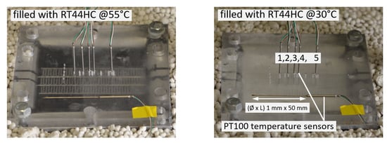
Figure 8.
Experimental tests with the thermally insulted HEX. The top plate is made from acryl glass.
Water is used as a heat transfer fluid. It is passed in concurrent flow at a relatively high flow rate of >290 L/h measured by Emerson Micro Motion ELITE Coriolis Meter CMF025M with transmitter 2700 (Emerson Electric Co., Ferguson, Missouri, U.S.). Therefore, and because of the relatively small amounts of heat transferred between water and PCM, constant water temperature is assumed in both liquid passages in the HEX. Water temperature is controlled by a Julabo FP51-SL (Ultra-Low Refrigerated-Heating Circulator) temperature control unit (Julabo Labortechnik, Seelbach, Germany) with a maximum heating and cooling thermal power of 3 and 2 kW, respectively.
The PCM temperatures are measured by class A/0 C, 3-wire PT 100 Ohm temperature sensors (Heinz H. Meßwiderstände GmbH, Elgersburg, Germany). The measurement error is ±0.15 − 0.35 K. The sensors are installed in one air passage as shown in Figure 7 and Figure 8. The temperature at the liquid passage outer surface is measured by PT 100 temperature sensors of the same accuracy, see Figure 7 for their position.
4.4. Heat Transfer Modeling and Model Validation
It is assumed that the heat transfer in the PCM domain in the HEX can be computed by solution of a one-dimensional transient heat conduction problem with phase change (see [17] for details):
where is modeled by different smooth phase transition functions as identified in Section 4.2.
These functions are shown in Figure 6, The values for 2.6 J/(g·K), 2.8 J/(g·K) and 224.9 J/g and 229.8 J/g for RT35HC and RT44HC, respectively. In Equation (16), and are the PCM’s thermal conductivity and density, respectively, and are assumed to be constant with = 0.2 W/(m·K) and = 770 kg/m (RT35HC) and = 780 kg/m (RT44HC). The distance between the two liquid passages is 10.4 mm. The five PT100 temperature sensors are installed at the midpoint, at 5.2 mm. In order to account for the increased heat transfer surface area by the offset strip fins, the PCM domain is reduced and defined from x = 0 mm to x = L = 0.95 mm. Initial and boundary conditions are defined as follows: The mean PCM temperature measured at is used for . At m, the values for in the Dirichlet boundary condition are the mean values of the recorded temperatures at the liquid passage outer surface. At x = L, the Neumann boundary (symmetry) condition is considered.
The model is implemented in MATLAB (MathWorks, Natick, MA, US) using a fixed grid spatial discretization in x with six elements. A central difference scheme is used for the discretization of the term for the conduction heat transfer. The results is a system of six ordinary differential equations (ODE’s) whose solution yields the PCM temperatures for each element. The ODE’s are solved using MATLAB’s ode15s solver with default absolute and relative error tolerance equal 1 × 10 and 1 × 10, respectively.
The model validation is done considering the mean of the five PCM temperatures measured between the two liquid passages, see Figure 7. The recorded values are compared with model predictions for the sixth (last) discrete element. The results are shown in Figure 9.
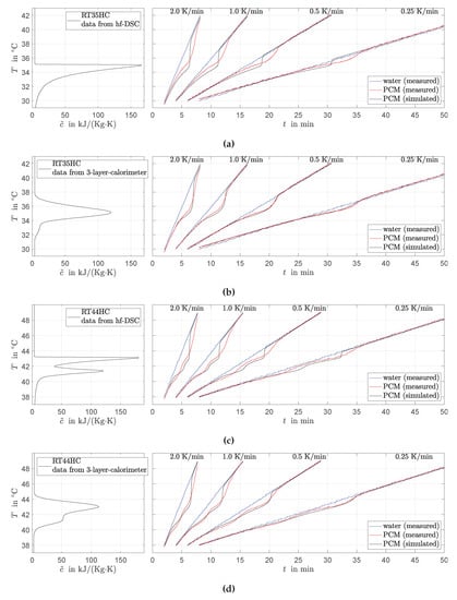
Figure 9.
Comparison of measured (exp.) and predicted (sim.) PCM temperatures in the HEX filled with RT35HC (a,b) and RT44HC (c,d) for different heating experiments where the water temperature is increased at different rates with 0.25 K/min, 0.5 K/min, 1.0 K/min, 2.0 K/min. Apparent specific heat capacities are taken from Figure 6.
The recorded PCM temperatures are clearly affected by the characteristic peak shapes of the apparent specific heat capacity . The deviation of the RT35HC temperature from the water temperature shows one increase followed by one decrease and occurs in the phase transition temperature range defined by the peak in (between 34 C and 37 C). It is noted that, for higher rates, this deviation is extended over a wider temperature range, and it ends later at higher temperatures. However, this behavior is also predicted by the model. It can be concluded that the (static) model for can be reasonably applied for different heating rates between 0.25 K/min and 2 K/min without losses in the prediction accuracy.
Both measured and predicted RT44HC temperatures are clearly affected by the two peaks in . The sharpness of the two peaks in derived from hf-DSC data leads to strongly pronounced responses (sudden changes in the course of predicted PCM temperatures). These effects are less present in the measured data. The phase transition model derived from 3-layer-calorimetry data fits the measured PCM temperatures better. The same is observed for the predicted and measured RT35HC temperatures. Table 2 reports the mean absolute and maximal differences between experimentally measured and predicted PCM temperatures. These values support all discussed results.
Table 2.
Mean absolute and maximal differences between experimentally measured and predicted PCM temperatures in the HEX. Differences are calculated from the data shown in Figure 9.
4.5. Performance of the Numerical Solver Using Either Discrete Signals or Smooth Functions
It is studied how the selection of either discrete signals (generated by numerical integration) or smooth functions (generated by spline interpolation) for modeling affects the efficiency of the numerical solution of the transient heat conduction problem in Equation (16). RT44HC is considered and the simulation problem is adapted as follows: The initial temperatures are C. At m, the Dirichlet boundary condition is defined by a sinusoidal function which oscillates around 41 C with an amplitude of 10 K and 1 min period of oscillation. At x = L = 0.01 m, the Neumann boundary condition is considered. 25 elements are used for the fixed grid spatial discretization in x. The problem is solved from t = 0 min to 5 min. The discrete signals (generated by the numerical integration method) cannot be directly used for modeling . They are first transformed into functions of a continuous argument (the temperature). This is realized by a table lookup with the following three different interpolation options provided by MATLAB: “nearest” neighbor interpolation, “linear” interpolation, and “pchip” piecewise cubic hermite interpolation.
The results are presented in Table 3. The reported solver statistics reflect the computational effort for solving the problem. They are given as: the number of “successful steps”, the number of “failed attempts”, the number of times the ODE model function was called to evaluate (“function evaluations”), and the number of “solutions of linear systems” of the implicit solver.
Table 3.
MATLAB’s ode15s solver statistics for the solution of the transient heat conduction problem in Equation (16).
For the phase transition functions from hf-DSC data, there is no clear differences between the performance when using either discrete signals or smooth functions. However, for the phase transition functions from 3-layer-calorimetry data, the computational effort is significantly lower when using smooth functions.
This can be explained by the sharp peak in the DSC signal between 43 C and 44 C, see Figure 4b. A possible explanation is that this sharp peak in makes the problem highly nonlinear and seems to dominate the problem complexity. Accordingly, the differences between discrete signals and smooth functions for do not lead to significant differences in the algorithm efficiency.
5. Discussion and Conclusions
The apparent heat capacity method is particularly suitable for the numerical modeling of heat transfer in technical-grade and mixed solid–liquid PCM’s. For these materials, phase transitions usually take place over an extended temperature range. In addition, sometimes more than one characteristic peak might be found in the heat capacity data. This is the case for RT44HC where two characteristic peaks could be clearly distinguished in DSC heat capacity data. These two peaks could be either the result of being a mixture of different compounds with different chain length, or of the possible occurrence of a solid–solid phase transition in addition to the solid–liquid transition. The two-phase apparent heat capacity method uses simplifying assumptions and considers one solid–liquid phase transition only. Corresponding phase transition models are defined by the following material properties: solid and liquid heat capacities, the phase transition enthalpy, and the phase fraction–temperature curve that defines the characteristic peak(s) in the apparent heat capacity curve. It is often recommendable to determine these characteristics individually. e.g., data from different measurement techniques and procedures, as well as different specific heating rates and sample volumes, might be used to determine the phase transition enthalpy, the heat capacities outside the phase transition temperature range, or the peak location and shape. The apparent heat capacity model accounts for an individual consideration of these properties.
The focus of this contribution is on the identification of phase fraction–temperature curves which accurately describe the phase transition behavior (peak shape and location) of commercial paraffin waxes filled in a compact HEX. The intended use case is the efficient numerical analysis of heat transfer in a (from the practical viewpoint reasonable) temperature operating range where significant heat is released or absorbed by the PCM.
PCM heat capacity data normally represent overall (apparent) heat capacities. Thus, the material properties need to be indirectly recovered from the data. The area-proportional baseline method generates phase fraction–temperature curves represented by discrete signals. These signals are not smooth and affected by noise in the measured heat capacity data. Therefore, their use is not recommendable for numerical modeling of heat transfer with differential equations. In contrast, the proposed spline interpolation method generates three times continuously differentiable ( smooth) phase transition functions. Derived apparent heat capacity and enthalpy models are smooth. Therefore, they are well suited for the efficient numerical solution of heat transfer problems in PCM (and corresponding dynamic optimization problems solved by derivative-based algorithms). This is confirmed by a simulation study. The statistics of the numerical solver show a significant reduction of computational effort by a factor of two or three when using smooth functions instead of discrete signals. It is noted that, for heat capacity data with very sharp peak signals (identified by hf-DSC at low temperature rates of 0.1 K/min), no reduction in the computational effort is found. These sharp peak signals make the simulation problem highly nonlinear and dominate its complexity. However, as discussed below, the heat capacity data from hf-DSC is not suitable for fitting PCM temperatures in a storage.
The splines adapt to the shape of the measured peak signals, i.e., no assumptions need to be taken on the curve shape. The accuracy of the interpolation scheme depends on the number of grid elements, the grid placement, and the peak shape. For RT35HC and RT44HC heat capacity data generated by hf-DSC and 3-layer-calorimetry, the computed phase transition enthalpy and the baseline are accurately determined. All errors are well below 3%.
The comparison between predicted and measured RT35HC and RT44HC temperatures in a compact extended surface HEX reveals significant differences in the accuracy of heat transfer models. If the models are linked with phase transition functions identified from hf-DSC data recorded at 0.1 K/min, the predictions strongly overestimate the characteristic features of the phase change, i.e., the sharpness of the melting peaks for RT35HC and RT44HC. In contrast, good results are obtained if the models are linked with functions identified from data from 3-layer-calorimetry. Here, the quality of the fitting is comparable to previous results for RT64HC, see Barz et al. [17], where data from 3-layer-calorimetry were used to predict PCM temperatures in a compact HEX of a similar design as the one used in this contribution. It can be concluded that, for the paraffin waxes RT35HC, RT44HC and RT64HC (filled in a compact extended surface HEX), the phase change behavior during heating (with moderate heating rates between 0.25 to 2.0 K/min) is well represented by the heat capacity data from 3-layer-calorimetry. Because of these promising results, the method is applied to melting data of all 44 Rubitherm paraffins. The computer code and a documentation of the corresponding phase transition models is provided in the supplementary information.
Finally, it is noted that all presented apparent heat capacity models are (temperature) rate-independent and are identified from heat capacity data for complete melting experiments. Further studies are conceivable which combine results from melting and solidification experiments at different temperature rates and which are directed to the prediction of both complete and incomplete phase transitions. This is especially interesting for the here considered solid–liquid PCM with a non-isothermal phase transition behavior, possibly with hysteresis, supercooling and varying phase fraction–temperature relationship.
Supplementary Materials
The following are available online at https://www.mdpi.com/1996-1073/13/19/5149/s1.
Author Contributions
Conceptualization, T.B.; methodology T.B. and J.E.; software, T.B.; formal analysis, data curation and visualization, T.B.; investigation, T.B. and J.K.; validation, T.B.; writing—original draft preparation, T.B.; writing—review and editing, T.B. and J.E.; supervision, T.B.; project administration, T.B. and J.E.; resources, T.B.; funding acquisition, J.E. and T.B. All authors have read and agreed to the published version of the manuscript.
Funding
This work has been supported by the FFG (Austrian Research Promotion Agency) through the project “WHole-Battery” (Grant No. 871546) in the program “Mobilität der Zukunft”.
Acknowledgments
The authors acknowledge the help of the European Union’s Horizon 2020 research and innovation program through the project “HYBUILD” (Grant No. 768824). The authors would also like to thank Birgo Nitsch and Andreas Strehlow (AKG Verwaltungsgesellschaft mbH, Hofgeismar, Germany) for fruitful discussion and provision of the aluminium HEX.
Conflicts of Interest
The authors declare no conflict of interest. The funders had no role in the design of the study; in the collection, analysis, or interpretation of data; in the writing of the manuscript, or in the decision to publish the results.
References
- Farid, M.M.; Khudhair, A.M.; Razack, S.A.K.; Al-Hallaj, S. A review on phase change energy storage: Materials and applications. Energy Convers. Manag. 2004, 45, 1597–1615. [Google Scholar] [CrossRef]
- Shukla, A.; Buddhi, D.; Sawhney, R.L. Thermal cycling test of few selected inorganic and organic phase change materials. Renew. Energy 2008, 33, 2606–2614. [Google Scholar] [CrossRef]
- Hadjieva, M.; Kanev, S.; Argirov, J. Thermophysical properties of some paraffins applicable to thermal energy storage. Sol. Energy Mater. Sol. Cells 1992, 27, 181–187. [Google Scholar] [CrossRef]
- Aydın, A.A.; Okutan, H. High-chain fatty acid esters of myristyl alcohol with even carbon number: Novel organic phase change materials for thermal energy storage—1. Sol. Energy Mater. Sol. Cells 2011, 95, 2752–2762. [Google Scholar] [CrossRef]
- Anghel, E.M.; Georgiev, A.; Petrescu, S.; Popov, R.; Constantinescu, M. Thermo-physical characterization of some paraffins used as phase change materials for thermal energy storage. J. Therm. Anal. Calorimetry 2014, 117, 557–566. [Google Scholar] [CrossRef]
- Agarwal, A.; Sarviya, R.M. Characterization of commercial grade paraffin wax as latent heat storage material for solar dryers. Mater. Today Proc. 2017, 4, 779–789. [Google Scholar] [CrossRef]
- Zmywaczyk, J.; Zbińkowski, P.; Smogór, H.; Olejnik, A.; Koniorczyk, P. Cooling of high-power led lamp using a commercial paraffin wax. Int. J. Thermophys. 2017, 38, 45. [Google Scholar] [CrossRef]
- Sam, M.N.; Caggiano, A.; Mankel, C.; Koenders, E. A Comparative Study on the Thermal Energy Storage Performance of Bio-Based and Paraffin-Based PCMs Using DSC Procedures. Materials 2020, 13, 1705. [Google Scholar]
- Voller, V.R.; Swaminathan, C.R. General source-based method for solidification phase change. Numer. Heat Transf. Part Fundam. 1991, 19, 175–189. [Google Scholar] [CrossRef]
- Voller, V.R.; Swaminathan, C.R.; Thomas, B.G. Fixed grid techniques for phase change problems: A review. Int. J. Numer. Methods Eng. 1990, 30, 875–898. [Google Scholar] [CrossRef]
- Gaur, U.; Wunderlich, B. Heat capacity and other thermodynamic properties of linear macromolecules. II. Polyethylene. J. Phys. Chem. Ref. Data 1981, 10, 119. [Google Scholar] [CrossRef]
- Barz, T.; Sommer, A. Modeling hysteresis in the phase transition of industrial-grade solid/liquid PCM for thermal energy storages. Int. J. Heat Mass Transf. 2018, 127, 701–713. [Google Scholar] [CrossRef]
- Voller, V.R.; Prakash, C. A fixed grid numerical modelling methodology for convection-diffusion mushy region phase-change problems. Int. J. Heat Mass Transf. 1987, 30, 1709–1719. [Google Scholar] [CrossRef]
- Brent, A.D.; Voller, V.R.; Reid, K.J. enthalpy–porosity technique for modeling convection-diffusion phase change: Application to the melting of a pure metal. Numer. Heat Transf. 1988, 13, 297–318. [Google Scholar] [CrossRef]
- Galione, P.A.; Lehmkuhl, O.; Rigola, J.; Oliva, A. Fixed-grid numerical modeling of melting and solidification using variable thermo-physical properties–Application to the melting of n-Octadecane inside a spherical capsule. Int. J. Heat Mass Transf. 2015, 86, 721–743. [Google Scholar] [CrossRef]
- Caggiano, A.; Mankel, C.; Koenders, E. Reviewing Theoretical and Numerical Models for PCM-embedded Cementitious Composites. Buildings 2019, 9, 3. [Google Scholar] [CrossRef]
- Barz, T.; Emhofer, J.; Marx, K.; Zsembinszki, G.; Cabeza, L.F. Phenomenological modelling of phase transitions with hysteresis in solid/liquid PCM. J. Build. Perform. Simul. 2019, 12, 770–788. [Google Scholar] [CrossRef]
- Goia, F.; Chaudhary, G.; Fantucci, S. Modeling and experimental validation of an algorithm for simulation of hysteresis effects in phase change materials for building components. Energy Build. 2018, 174, 54–67. [Google Scholar] [CrossRef]
- Mankel, C.; Caggiano, A.; Ukrainczyk, N.; Koenders, E. Thermal energy storage characterization of cement-based systems containing microencapsulated-PCMs. Constr. Build. Mater. 2019, 199, 307–320. [Google Scholar] [CrossRef]
- FLUENT Manual. Chapter 21: Modeling Solidification and Melting; Technical Report; ANSYS, Inc.: Canonsburg, PA, USA, 2001. [Google Scholar]
- Diaconu, B.M.; Cruceru, M. Novel concept of composite phase change material wall system for year-round thermal energy savings. Energy Build. 2010, 42, 1759–1772. [Google Scholar] [CrossRef]
- Delcroix, B. Modeling of Thermal Mass Energy Storage in Buildings With Phase Change Materials. Ph.D. Thesis, École Polytechnique de Montréal, Montréal, QC, Canada, 2015. [Google Scholar]
- Virgone, J.; Trabelsi, A. 2D Conduction simulation of a PCM storage coupled with a heat pump in a ventilation system. Appl. Sci. 2016, 6, 193. [Google Scholar] [CrossRef]
- Michel, B.; Glouannec, P.; Fuentes, A.; Chauvelon, P. Experimental and numerical study of insulation walls containing a composite layer of PU-PCM and dedicated to refrigerated vehicle. Appl. Therm. Eng. 2017, 116, 382–391. [Google Scholar] [CrossRef]
- Biswas, K.; Shukla, Y.; Desjarlais, A.; Rawal, R. Thermal characterization of full-scale PCM products and numerical simulations, including hysteresis, to evaluate energy impacts in an envelope application. Appl. Therm. Eng. 2018, 138, 501–512. [Google Scholar] [CrossRef]
- Moreles, E.; Huelsz, G.; Barrios, G. Hysteresis effects on the thermal performance of building envelope PCM-walls. Build. Simul. 2018, 11, 519–531. [Google Scholar] [CrossRef]
- Hu, Y.; Heiselberg, P.K. A new ventilated window with PCM heat exchanger—Performance analysis and design optimization. Energy Build. 2018, 169, 185–194. [Google Scholar] [CrossRef]
- Andrássy, Z.; Szánthó, Z. Thermal behaviour of materials in interrupted phase change. J. Therm. Anal. Calorim. 2019, 138, 3915–3924. [Google Scholar] [CrossRef]
- Zukowski, M. Mathematical modeling and numerical simulation of a short term thermal energy storage system using phase change material for heating applications. Energy Convers. Manag. 2007, 48, 155–165. [Google Scholar] [CrossRef]
- Franquet, E.; Gibout, S.; Bédécarrats, J.P.; Haillot, D.; Dumas, J.P. Inverse method for the identification of the enthalpy of phase change materials from calorimetry experiments. Thermochim. Acta 2012, 546, 61–80. [Google Scholar] [CrossRef]
- Kumarasamy, K.; An, J.; Yang, J.; Yang, E.H. Numerical techniques to model conduction dominant phase change systems: A CFD approach and validation with DSC curve. Energy Build. 2016, 118, 240–248. [Google Scholar] [CrossRef]
- Kumarasamy, K.; An, J.; Yang, J.; Yang, E.H. Novel CFD-based numerical schemes for conduction dominant encapsulated phase change materials (EPCM) with temperature hysteresis for thermal energy storage applications. Energy 2017, 132, 31–40. [Google Scholar] [CrossRef]
- Gowreesunker, B.L.; Tassou, S.A.; Kolokotroni, M. Improved simulation of phase change processes in applications where conduction is the dominant heat transfer mode. Energy Build. 2012, 47, 353–359. [Google Scholar] [CrossRef]
- Gowreesunker, B.L.; Tassou, S.A. Effectiveness of CFD simulation for the performance prediction of phase change building boards in the thermal environment control of indoor spaces. Build. Environ. 2013, 59, 612–625. [Google Scholar] [CrossRef][Green Version]
- Mehling, H.; Barreneche, C.; Solé, A.; Cabeza, L.F. The connection between the heat storage capability of PCM as a material property and their performance in real scale applications. J. Energy Storage 2017, 13, 35–39. [Google Scholar] [CrossRef]
- Noël, J.A.; Kahwaji, S.; Desgrosseilliers, L.; Groulx, D.; White, M.A. Phase change materials. In Storing Energy; Elsevier: Amsterdam, The Netherlands, 2016; pp. 249–272. [Google Scholar]
- Klimeš, L.; Charvát, P.; Joybari, M.M.; Zálešák, M.; Haghighat, F.; Panchabikesan, K.; El Mankibi, M.; Yuan, Y. Computer modelling and experimental investigation of phase change hysteresis of PCMs: The state-of-the-art review. Appl. Energy 2020, 263, 114572. [Google Scholar] [CrossRef]
- Günther, E.; Mehling, H.; Hiebler, S. Modeling of subcooling and solidification of phase change materials. Model. Simul. Mater. Sci. Eng. 2007, 15, 879. [Google Scholar] [CrossRef]
- Uzan, A.Y.; Kozak, Y.; Korin, Y.; Harary, I.; Mehling, H.; Ziskind, G. A novel multi-dimensional model for solidification process with supercooling. Int. J. Heat Mass Transf. 2017, 106, 91–102. [Google Scholar] [CrossRef]
- Davin, T.; Lefez, B.; Guillet, A. Supercooling of phase change: A new modeling formulation using apparent specific heat capacity. Int. J. Therm. Sci. 2020, 147, 106121. [Google Scholar] [CrossRef]
- Jin, X.; Hu, H.; Shi, X.; Zhou, X.; Yang, L.; Yin, Y.; Zhang, X. A new heat transfer model of phase change material based on energy asymmetry. Appl. Energy 2018, 212, 1409–1416. [Google Scholar] [CrossRef]
- Hemminger, W.; Sarge, S. The baseline construction and its influence on the measurement of heat with differential scanning calorimeters. J. Therm. Anal. Calorim. 1991, 37, 1455–1477. [Google Scholar] [CrossRef]
- Höhne, G.; Flemminger, W.; Flammersheim, H.J. Differential Scanning Calorimetry; Springer: Berlin/Heidelberg, Germany; New York, NY, USA, 2003. [Google Scholar]
- Bandara, U. A systematic solution to the problem of sample background correction in DSC curves. J. Therm. Anal. 1986, 31, 1063–1071. [Google Scholar] [CrossRef]
- DIN 51007. Thermische Analyse (TA)–Differenz-Thermoanalyse (DTA) und Dynamische Differenzkalorimetrie (DSC): Allgemeine Grundlagen; German Institute for Standardisation (Deutsches Institut für Normung): Berlin, Germany, 2019. [Google Scholar]
- Roduit, B.; Borgeat, C.; Berger, B.; Folly, P.; Alonso, B.; Aebischer, J.N.; Stoessel, F. Advanced kinetic tools for the evaluation of decomposition reactions: Determination of thermal stability of energetic materials. J. Therm. Anal. Calorim. 2005, 80, 229–236. [Google Scholar] [CrossRef]
- Diaconu, B.M.; Varga, S.; Oliveira, A.C. Experimental assessment of heat storage properties and heat transfer characteristics of a phase change material slurry for air conditioning applications. Appl. Energy 2010, 87, 620–628. [Google Scholar] [CrossRef]
- Gschwander, S.; Haussmann, T.; Hagelstein, G.; Sole, A.; Cabeza, L.F.; Diarce, G.; Hohenauer, W.; Lager, D.; Ristic, A.; Rathgeber, C.; et al. Standardization of PCM Characterization via DSC; IEA ECES Greenstock: Beijing, China, 2015. [Google Scholar]
- Lindenberg, G.; Laube, A. Das 3-Schicht-Kalorimeter-Ein einfaches, aber präzises Verfahren zur Bestimmung der Speicherkapazität von Latentwärmespeichermaterial. Available online: http://www.waermepruefung.de/projekte_messsystem_kalorimeter.html (accessed on 30 September 2020).
- Kenfack, F.; Bauer, M. Innovative Phase Change Material (PCM) for heat storage for industrial applications. Energy Procedia 2014, 46, 310–316. [Google Scholar] [CrossRef]
- Vidi, S.; Mehling, H.; Hemberger, F.; Haussmann, T.; Laube, A. Round-Robin test of paraffin phase-change material. Int. J. Thermophys. 2015, 36, 2518–2522. [Google Scholar] [CrossRef]
- Laube, A.; (Bern University of Applied Sciences, Fürstenwalde/Spree, Germany). Personal communication, 2020.
- Mehling, H.; Cabeza, L.F. Heat And Cold Storage With PCM: An Up To Date Introduction Into Basics and Applications; Springer: Cham, Switzerland, 2008. [Google Scholar]
© 2020 by the authors. Licensee MDPI, Basel, Switzerland. This article is an open access article distributed under the terms and conditions of the Creative Commons Attribution (CC BY) license (http://creativecommons.org/licenses/by/4.0/).