An Approach to Detecting Cyber Attacks against Smart Power Grids Based on the Analysis of Network Traffic Self-Similarity

Abstract

The paper discusses an approach for detecting cyber attacks against smart power supply networks, based on identifying anomalies in network traffic by assessing its self-similarity property. Methods for identifying long-term dependence in fractal Brownian motion and real network traffic of smart grid systems are considered. It is shown that the traffic of a telecommunication network is a self-similar structure, and its behavior is close to fractal Brownian motion. Fractal analysis and mathematical statistics are used as tools in the development of this approach. The issues of a software implementation of the proposed approach and the formation of a dataset containing network packets of smart grid systems are considered. The experimental results obtained using the generated dataset have demonstrated the existence of self-similarity in the network traffic of smart grid systems and confirmed the fair efficiency of the proposed approach. The proposed approach can be used to quickly detect the presence of anomalies in the traffic with the aim of further using other methods of cyber attack detection.

1. Introduction

The modern electric power systems are highly developed systems with a multi-level hierarchical structure [1]. For the “smart control” of such a complex, ramified, and non-linear system, the search and use of innovative approaches for predicting the network events in order to generate the right and operational solutions are necessary.

The main trend influencing the development of information systems in the energy sector is the smart grid (SG) concept. The energy system based on the SG concept is a single energy and information complex, where managed objects should allow remote control, and the situation assessment and emergency automation systems should reduce excessive requirements for power and information capacity reserves.

The emergence of such a system is an opportunity, at the expense of new means and a new organization to control the functioning and development of the intelligent energy system, to provide new properties and new effects. These new properties and new effects are as follows: survivability; power quality [2]; the possibility of its accumulation; management of intersystem flows and the removal of unnecessary restrictions on the synchronous operation of all parts of the system; segmentation and hierarchy of power energy and information flows; distribution of management decisions (current and prospective) and responsibility for them; optimization of primary energy resources and investments used; as well as expanded reproduction of production and financial assets, the country’s total energy potential [3].

However, the use of information and communication networks and technologies in SG to collect information about energy production and energy consumption, on the one hand, increases the efficiency, reliability, economic benefit, and stability of electricity production and distribution, and on the other hand, enables an attacker to influence SG by implementing cyber attacks [4]. The impact of cyber attacks is possible due to the mass use of outdated operating systems and applications, inefficient protection mechanisms, and the presence of multiple vulnerabilities in network protocols. Using such vulnerabilities gives a potential attacker the ability to change network device settings, listen and redirect traffic, block network interaction, and gain unauthorized access to internal components of industrial systems.

The impact of cyber attacks leads to the appearance of abnormal traffic activity in SG. For continuous monitoring and detection of anomalous activity of traffic in SG, it is necessary to take into account the presence of a large number of network routes, which periodically cause sharp fluctuations in the delay of data transmission and large packet loss, the emergence of new properties of network traffic, as well as the need to ensure high-quality application service [5]. All this serves as an occasion to search for new methods for detecting and predicting cyber attacks [6,7,8,9], which include fractal analysis.

The presence of fractal properties of network traffic was discovered several decades ago, when it was found that on a large scale, it has the property of self-similarity, that is, it looks qualitatively the same with a sufficiently large scale of the time axis and exhibits a long-term dependence [10]. Previously dominant traffic models based on the Markov processes have a short-term dependence. They are borrowed from telephone networks and, as applied to computer networks, leads to an underestimation of the load.

Fractal analysis, as a method of studying mathematical sets of various natures, is based on the ideas of fractal geometry developed by B. Mandelbrot. Since 1973, when his fundamental work was published, fractal analysis methods have been widely used in various fields of physics, chemistry, and biology. The main achievement of the theory of fractals is that it provides simple methods for the mathematical description of very complex but very widespread in natural phenomena and objects. Fractal analysis is an equally fundamental mathematical apparatus for describing physical reality as differential equations, trigonometry, or harmonic analysis. However, due to the fact that it has been discovered relatively recently, it has not yet taken its rightful place in the minds of scientists and engineers. Therefore, the work demonstrating the range of possible applications of fractal analysis for detecting cyber attacks against information and communication networks in SG is undoubtedly relevant.

The contribution of this paper is as follows: (1) the structures of long-term dependencies in SG traffic are investigated, making it possible to reveal its characteristic features in the interests of early detection of cyber attacks; (2) a new approach to the detection of cyber attacks based on the analysis of the fractal properties of traffic is proposed; (3) a software prototype is developed that implements the proposed approach, and a dataset with SG traffic containing anomalies from the impact of cyber attacks is generated; (4) an experimental evaluation of the proposed approach is carried out, showing its rather high efficiency.

The novelty of the obtained results lies in the fact that, on the basis of experimental studies, the efficient method for determining self-similarity for non-stationary time series has been substantiated, which allows, with high accuracy and fairly quickly, one to detect changes in traffic that may correspond to the initial stages of the implementation of various cyber attacks, such as “Distributed Denial-of-Service” (DDoS), “Scanning the network and its vulnerabilities”, and others. This is a significant advantage of the proposed method.

The further structure of the paper is as follows. Section 2 reviews relevant papers on the research topic. Section 3 describes the theoretical foundations of the proposed approach to detecting cyber attacks based on the analysis of fractal properties of traffic. This section discusses the basic concepts of the theory of fractals, the main methods for determining the Hurst exponent, such as the extended Dickey–Fuller test, rescaled range (R/S) analysis, and the detrended fluctuation analysis (DFA) method, and also provides a general description of the proposed method for detecting cyber attacks based on the fractal approach. Section 4 presents the implementation issues of the proposed approach, including a description of the dataset used for the experiments. Section 5 outlines the results of an experimental evaluation of the proposed approach and its comparative evaluation with other approaches and methods for detecting cyber attacks. Section 6 contains the main conclusions on the work and directions for further research.

2. Related Work

At present, the issues related to the study of self-similar properties of time series and their practical application in various monitoring systems are in the focus of the attention of many researchers. Fractal properties are investigated in many works. Thus, in [11], the R/S-analysis method is used to identify patterns in time series. In [12], the VoIP traffic is modeled, and its fractal properties are also investigated. In [13], not only the Hurst exponent is studied but also the fractal dimension. In [14], the authors explain why teletraffic has fractal properties. However, these works mainly cover the financial sector and VoIP telephony.

It should be noted that there are few practical experiments aimed at studying the fractal properties of network traffic in telecommunication systems. Among this kind of work, one can single out the papers [15,16,17]. However, in [15], traffic is considered not in information and telecommunication networks, but in radio waves transmitted by cellular stations. In addition, researchers come to the conclusion that movement is self-similar, often relying solely on visual signs [16,17]. They look for similar areas on the chart, passing them off as self-similar processes.

One of the first works, which considers the property of self-similarity of network traffic, is [10]. In it, the existing ideas about the processes occurring in information and telecommunication networks have been changed significantly. This view has been discussed in more detail in the next section. It is also necessary to highlight a number of works proposing the mathematical models that describe the fractal properties of network traffic, for example, [18,19]. However, they are not focused on detecting cyber attacks, and they cannot be considered exhaustive. Thus, our paper, on the one hand, is based on the progress achieved in the study of self-similar properties of telecommunication traffic. On the other hand, it develops further known solutions towards creating a method that allows detecting network traffic anomalies caused by the impact of cyber attacks.

3. Theoretical Foundations of the Suggested Approach to Cyber Attack Detection

3.1. Basic Concepts of Fractal Theory

A key parameter of fractal analysis is the Hurst exponent. This is a measure that is used in time series analysis. The greater the delay between the two identical pairs of values in a time series, the lower the Hurst exponent (scaling index). To find this parameter, it is necessary to know whether the process under study is stationary. Whether it is stationary or not depends on the choice of the algorithm for further scaling calculation [11,12,13].

In practice, random processes are very common, occurring in time approximately uniformly and having the form of continuous random oscillations around a certain average value. In this case, neither the average amplitude nor the nature of these oscillations shows significant changes over time. Such random processes are called stationary.

A random process $X\left(t\right)$ is called stationary if its mathematical expectation $m_x\left(t\right)$ is a constant number, and the correlation function $K_x\left(t_1,t_2\right)$ depends only on the difference of the arguments, i.e., $m_x\left(t\right)=m=\mathrm{const}$; $K_x\left(t_1,t_2\right)=K_x\left(t_2-t_1\right)$. It follows from this that the correlation function of the stationary process is a function of one argument: $K_x\left(t_1,t_2\right)=K_x\left(\mathsf{\tau }\right)$, $\mathsf{\tau }=t_2-t_1$. This circumstance often simplifies operations on stationary processes.

An example of a stationary process is white noise. Stationary white noise is a stationary process $X\left(t\right)$, whose spectral density is a constant number: $S_X^{*}\left(\mathsf{\omega }\right)=S_0=\mathrm{const}$ for $\forall \mathsf{\omega }\in \left(-\infty ,+\infty \right)$.

When the time series is stationary, it is easier to model. Statistical modeling methods assume or require that the time series should be stationary in order to be effective.

An example of a non-stationary process is the fractal Brownian motion (FBM), which is widely used in various sciences.

A Gaussian process $X\left(t\right)$ is called a fractal Brownian motion with the parameter H (the Hurst exponent), if the increments of a random process $\mathsf{\Delta }X\left(\mathsf{\tau }\right)=X\left(t+\mathsf{\tau }\right)-X\left(t\right)$ have a Gaussian distribution:

$$P\left(\mathsf{\Delta }X<x\right)=\frac{1}{\sqrt{2\mathsf{\pi }}{\mathsf{\delta }}_0{\mathsf{\tau }}^H}{\displaystyle \underset{-\infty }{\overset{x}{\int }}\exp \left[-\frac{z^2}{2{\mathsf{\delta }}_0^2{\mathsf{\tau }}^{2H}}\right]}dz,$$

(1)

where ${\mathsf{\delta }}_0$ is the diffusion coefficient.

The fractal Brownian motion with the parameter $H=\frac{1}{2}$ coincides with the classical Brownian motion [14,15]. Thus, in order to detect cyber attacks, it is initially necessary to determine the type of traffic-stationary or non-stationary. Next, it is needed to calculate the Hurst exponent (i.e., determine the presence of self-similarity in traffic). Finally, anomalies should be detected.

Below are the main methods for performing all these stages of cyber attack detection.

3.2. Dickey–Fuller Augmented Test

There are many additional tests for checking stationarity. One of the most common tests is the Dickey–Fuller test.

The augmented Dickey–Fuller test (ADF) is used in applied statistics and econometrics to analyze time series to test for stationarity. It was proposed by David Dickey and Wayne Fuller [16].

Let the data be generated by the following process: $\mathsf{\Delta }{y}_t=b{y}_{t-1}+{\mathsf{\epsilon }}_t$, where $b=a-1$, and $\mathsf{\Delta }$ is the first-order difference operator $\mathsf{\Delta }{y}_t=y_{t-1}-y_{t-1}$. Therefore, testing the unit root hypothesis in this representation means checking the null hypothesis that the coefficient $b$ is equal to zero. Since the case of “explosive” processes is excluded, the test is one-sided, that is, an alternative hypothesis is a hypothesis that the coefficient $b$ is less than zero. Test statistics (Dickey–Fuller or DF statistics) are common t-statistics for checking the significance of linear regression coefficients. However, the distribution of DF statistics is expressed through the Wiener process and is called the Dickey–Fuller distribution.

There are three versions of the test regressions (here $b_0$ is a constant, $b_1$ and $b$ are linear coefficients, and ${\mathsf{\epsilon }}_t$ is a bias):

(1)

Without constant and trend $\mathsf{\Delta }{y}_t=b{y}_{t-1}+{\mathsf{\epsilon }}_t$.

(2)

With a constant, but no trend $\mathsf{\Delta }{y}_t=b_0+b{y}_{t-1}+{\mathsf{\epsilon }}_t$.

(3)

With a constant and linear trend $\mathsf{\Delta }{y}_t=b_0+b_{1}t+b{y}_{t-1}+{\mathsf{\epsilon }}_t$.

Each of the three test regressions has its own critical values of DF statistics, which are taken from a special Dickey–Fuller (McKinnon) table. If the statistic value lies to the left of the critical value at a given significance level (i.e., critical values are negative), then the null hypothesis of a unit root is rejected. The process is considered stationary (in the sense of this test). Otherwise, the hypothesis is not rejected. In this case, the process can contain unit-roots, and it is a non-stationary (integrated) time series.

If lags of the first differences of the time series are added to test regressions, then the distribution of DF statistics (and, therefore, critical values) will not change. Such a test is called the ADF test. The need to include lags of the first differences is due to the fact that the process may not be autoregression of the first, but of a higher order [17,18,19].

An obvious disadvantage of the Dickey–Fuller test is the fact that it does not take into account possible autocorrelation in residuals. If autocorrelation is observed in the residuals, then the results of the usual least-squares method will be unreliable. In this case, it is necessary to consider other methods of fractal analysis, in which this drawback is eliminated.

Thus, the extended Dickey–Fuller test is a means of checking the stationarity of the traffic time series. To test traffic for stationarity, it is necessary to use the standard hypothesis testing procedure using tables of critical values for the Dickey–Fuller distribution. Since the Dickey–Fuller statistics allow only checking for stationarity, we have considered methods for finding the Hurst exponent.

3.3. R/S Analysis

The rescaled range (R/S) analysis algorithm consists of eight steps. The original time series is divided into blocks of the same length. For each block, the amplitude R and standard deviation S are calculated. Then, the average $R/S$ ratio is found for all blocks. The block size is increasing. The algorithm is repeated again until the block size is equal to the size of the original time series. As a result, an average $R/S$ is obtained for each block size. Performing a least-squares regression, we can find $H$. Each step of the R/S analysis algorithm is described in more detail.

• Let there be a sample of length $X$. This sample is a time series in which the number of observations is quite high (usually more than 5000). We transform the sample into a time series of length $N=X-1$ using the following logarithmic relations:

  $$N_i=\ln \frac{X_i}{X_{i-1}},i=1,2,\dots ,\left(X-1\right).$$

  (2)
• The resulting time series $N$ is divided into several periods $k_i$ in such a way that

  $$N=k_i\mathsf{\tau },$$

  (3)

  where i is the period number; τ is the period length.
• Each item is marked with an index l = 1, 2, …, τ.
  For each $k_i$ of length τ, the average value is determined as follows:

  $$e_i=\frac{1}{\mathsf{\tau }}{\displaystyle \sum _{l=1}^n{N}_{l,i}}.$$

  (4)
• The time series of accumulated deviations $X_{l,i}$ from the average value for each sub-period $k_i$ is determined as follows:

  $$X_{l,i}={\displaystyle \sum _{j=1}^l\left(k_{j,i}-e_i\right)},$$

  (5)

  where $k_{j,i}$ is the value of the j-th sample in the sub-period $k_i$.
• The range is defined as the maximum value $X_{l,i}$ minus the minimum value $X_{l,i}$ within each sub-period $k_i$:

  $$R_{k_i}=\max \left(X_{l,i}\right)-\min \left(X_{l,i}\right),1\le l\le \mathsf{\tau }.$$

  (6)
• The sample standard deviation calculated for each sub-period $k_i$ is

  $$S_{k_i}=\frac{\sqrt{{\displaystyle \sum _{l=1}^n{\left(k_{l,i}-e_i\right)}^2}}}{\mathsf{\tau }-1}.$$

  (7)
• Each range $R_{k_i}$ is now normalized by dividing by the corresponding $S_{k_i}$. Therefore, the re-normalized range during each sub-period $k_i$ is equal to $R_{k_i}/S_{k_i}$. In step 2 above, we have obtained adjacent sub-periods of length τ. Therefore, the average value of $R/S$ for length τ is defined as:

  $${\left(R/S\right)}_{\mathsf{\tau }}=\frac{\mathsf{\tau }\cdot {\displaystyle \sum _{i=1}^{\frac{N}{\mathsf{\tau }}}{\left(R/S\right)}_{k_i}}}{N}.$$

  (8)
  The length n increases to the next higher value, and ${\left(M-1\right)}_{\mathsf{\tau }}$ is an integer value. We use values $\mathsf{\tau }$ that include the start and end points of the time series. Steps 1–6 are repeated until $\mathsf{\tau }=\frac{\left(M-1\right)}{2}$.
• Now the equation $\ln \left(R/S\right)=\ln \left(c\right)+H\ln \left(\mathsf{\tau }\right)$ can be applied by performing a simple least-squares regression on $\ln \left(\mathsf{\tau }\right)$ as an independent variable, and $\ln \left(R/S\right)$ as a dependent variable, where $R$ is the maximum range of the series under study, $S$ is the standard deviation of the observations, and $n$ is the number of observations [10,20].

3.4. DFA

The detrended fluctuation analysis (DFA) method allows one to calculate the Hurst exponent for different analysis depths $\mathsf{\tau }$. DFA is effective in finding the Hurst exponent in long-memory processes using a fluctuation function $F\left(n\right)$. First, we distinguish the fluctuation profile from the series $x\left(k\right)$:

$$Y\left(i\right)={\displaystyle \sum _{k=1}^i\left|x\left(k\right)-\overline{x}\right|},\mathrm{where}\overline{x}\mathrm{is}\mathrm{the}\mathrm{average}\mathrm{value}\mathrm{of}\mathrm{series}x\left(k\right).$$

(9)

Then, we divide the obtained values $Y\left(i\right)$ into segments of length $n$, the number of which is equal to an integer:

$$N_n=\frac{N}{n}.$$

(10)

Since the length of the series $N$ is not always a multiple of the chosen scale $n$, in the general case, the last section contains the number of points less than $n$. To account for this residue, it is necessary to repeat the procedure of dividing into segments, starting from the opposite end of the row.

As a result, the total number of segments with length $n$ will be $2N_n$.

Since the change in the random variable $Y\left(i\right)$ occurs near the value $Y_j\left(i\right)\ne 0$ due to a certain evolutionary trend of the series, we should find the local trend $Y_j\left(i\right)$ for each of $2N_n$ segments. In this case, it is easiest to use the least-squares method, representing the trend $Y_j\left(i\right)$ as a polynomial, the degree of which is chosen in such a way as to ensure interpolation with an error not exceeding the specified limit.

Then, we determine the variance:

$$F^2\left(j,n\right)=\frac{1}{n}{\displaystyle \sum _{i=1}^n{\left\{Y\left(\left(j-1\right)n+i\right)-Y_j\left(i\right)\right\}}^2}.$$

(11)

This expression is valid for the forward segments for which $j=1,\dots ,N_n$. For the reverse sequence, it is true $j=\left(N_n+1\right),\dots ,2N_n$. As a result, for the reverse sequence, we obtain the following expression for calculating the variance:

$$F^2\left(j,n\right)=\frac{1}{n}{\displaystyle \sum _{i=1}^n{\left\{Y\left(N-\left(j-N_n\right)n+i\right)-Y_j\left(i\right)\right\}}^2}.$$

(12)

The standard deviations (fluctuations) of the calculated integrated sequence relative to the local trend for the j-th interval are calculated by the formula

$$F\left(n\right)={\left\{\frac{1}{2N_n}{\displaystyle \sum _{j=1}^{2N_n}{F}^2\left(j,n\right)}\right\}}^{1/2}.$$

(13)

If the series under investigation reduces to a self-similar set, exhibiting long-range correlations, then the fluctuation function $F\left(n\right)$ is represented by a power-law dependence:

$$F\left(n\right)~n^H,$$

(14)

where $H$ is the Hurst exponent. $H$ can be calculated as the slope of the line that determines the dependencies $\log F\left(n\right)$ on $\log \left(n\right)$.

When $0.5<H<1$, a series is called persistent (subsequent changes in the values of the time series inherit its previous behavior). The process has a long memory.

At $H=0.5$, the series will be random (subsequent values of the time series are not related to its previous values).

When $0<H<0.5$, the series will be antipersistent (subsequent changes in the values of the time series are opposite to its previous behavior). The probability that at an $\left(i+1\right)$ step, the process deviates from the average in the opposite direction (with respect to the deviation at the i-th step) is as high as the parameter $H$ is close to 0 [10,18,21,22].

Thus, DFA is one of the universal approaches to identifying traffic self-similarity and is a universal method for processing measurement series. The DFA method is a variant of analysis of variance that allows one to study the effects of long-term correlations in non-stationary and stationary traffic. In this case, the root-mean-square error of the linear approximation is analyzed depending on the size of the approximation segment.

3.5. General Description of the Method for Detecting Cyber Attacks

The proposed method for detecting cyber attacks contains two stages.

At the first (auxiliary) stage, the analysis of the self-similar properties of the reference network traffic is performed. There are no anomalies in the reference traffic. As a result of this analysis, the value of the Hurst exponent is determined, corresponding to the reference traffic. This stage can be called the learning (training) stage. To determine the values of the Hurst exponent, the above methods of testing Dickey–Fuller, R/S analysis, and DFA are used.

At the second (main) stage, the self-similar properties of real traffic, in which anomalies caused by the impact of cyber attacks can exist, are analyzed. In this case, the methods discussed above for determining the values of the Hurst exponent are also used. If the identified value of the Hurst exponent differs from this value obtained for the reference traffic, a decision is made on the presence of anomalies in real traffic that may be caused by the impact of cyber attacks. In addition, at the same stage, the minimum size of the packet group, sufficient for an accurate assessment of the self-similarity index, is determined. The smaller the size of this group, the less time it takes to detect a cyber attack.

4. Software Implementation

The software implementation of the proposed cyber attack detection method is performed in Python using the following libraries and tools: Pandas, NumPy, Matplotlib, and Jupiter Notebook. The Pandas library enables high-level pivot tables, grouping and other table manipulations, and easy access to tabular data. The NumPy library is a low-level tool for working with high-level math functions as well as multidimensional arrays. The Matplotlib module provides graphing from the received dataset. Jupiter Notebook serves as a framework for calculations.

The algorithms that describe the two used methods, namely the ADF test and R/S analysis, as an example of a software implementation of the proposed method, are demonstrated.

A generalized algorithm for the augmented Dickey–Fuller test is outlined as Algorithm 1.

Algorithm 1. Augmented Dickey–Fuller Test

Input: The test dataset (x); maximum lag included in the test regression (maxlag); an order to include in regression (regression); the method to automatically determining the lag (autolag); the flag of returning to the adf statistic (store); the flag of the full regression results (regresults).

Output: A dummy class with results attached as attributes: the test statistic (adf); the number of lags used (usedlag); p-value (pvalue); critical values for the test statistic at the 1%, 5%, and 10% levels (critvalues). A dummy class with results attached as attributes (resstore).

01 Begin

02 if store = True then

03 maxlag = None; regression = “c”; autolag = “AIC”; regresults = False;

04 adf, pvalue = Adfuller (x, maxlag, regression, autolag, store, regresults);

05 critvalues = {critvalues [0] = “1%”, critvalues [1] = “5%”, critvalues [2] = “10%”},

06 resstore = ResultsStore (adf);

07 return adf, pvalue, critvalues, restore;

08 End

The input of Algorithm 1 is the following data: x, maxlag, regression, autolag, store, and regresults. The parameter regression can take the following values: “c” if constant only (default); “ct” if constant and trend; “ctt” if constant or linear and quadratic trend; “nc” if no constant, no trend. The parameter autolag can take the following values: “None” if the number of lags is used equal to maxlag; “AIC” (default) or “BIC” if the number of lags is chosen to minimize the corresponding information criterion; “t-stat” if choosing maxlag. In the latter case, the algorithm starts with the maxlag value, which decreases until the t-statistic at the last lag length becomes significant using the 5% test. If the store is equal to True, then a result instance is returned additionally to the adf statistic (default is False). If regresults is equal to True, then the full regression results are returned (default is False).

The null hypothesis of the augmented Dickey–Fuller test is that there is a unit root, with the alternative that there is no unit root. If the p-value pvalue is above a critical size, then we cannot reject that there is a unit root. The p-values are obtained through regression surface approximation by the library function Adfuller. If the p-value is close to significant, then the critical values should be used to judge whether to reject the null. This decision is made using the library function ResultsStore.

A generalized algorithm for the R/S analysis is represented as Algorithm 2.

Algorithm 2. R/S Analysis

Input: Time series (data).

Output: Hurst exponent (H) in the rescaled range approach for a given n.

01 Begin

02 total_N = len (data);

03 if total_N > 5000 then

04 m = total_N/n; // number of subsequences

05 data = data [total_N–(total_N% n)]; // cut values at the end of data to make the array divisible by n

06 np = data;

07 seqs = np.reshape (data, (m, n)); // split remaining data into subsequences of length n

08 means = np.mean (seqs, axis = 1); // calculate means of subsequences

09 y = seqs–means.reshape ((m, 1)); // normalize subsequences by substracting mean

10 y = np.cumsum (y, axis = 1); // build cumulative sum of subsequences

11 r = np.max (y, axis = 1)–np.min (y, axis = 1); // find ranges

12 s = np.std (seqs, axis = 1, ddof = 1 if unbiased else 0); // find standard deviation

13 idx = np.where (r!= 0); // some ranges may be zero and have to be excluded from the analysis

14 r = r [idx];

15 s = s [idx];

16 H = np.mean (r/s);

17 return H;

18 End

The calculation of H in Algorithm 2 is performed by the preliminary calculation of the parameters r and s. To do this, first, the time-series data is divided into m subsequences of length n. The algorithm then calculates the means of subsequences, normalizes them by subtracting the mean, and calculates the cumulative sums. After that, the standard deviation is found, and the parameters r and s are calculated. This process uses the standard functions of the Pandas library for working with tables (reshape, mean, cumsum, max, mix, and where). Finally, the parameter H is calculated as the average of the ratio obtained by dividing r by s.

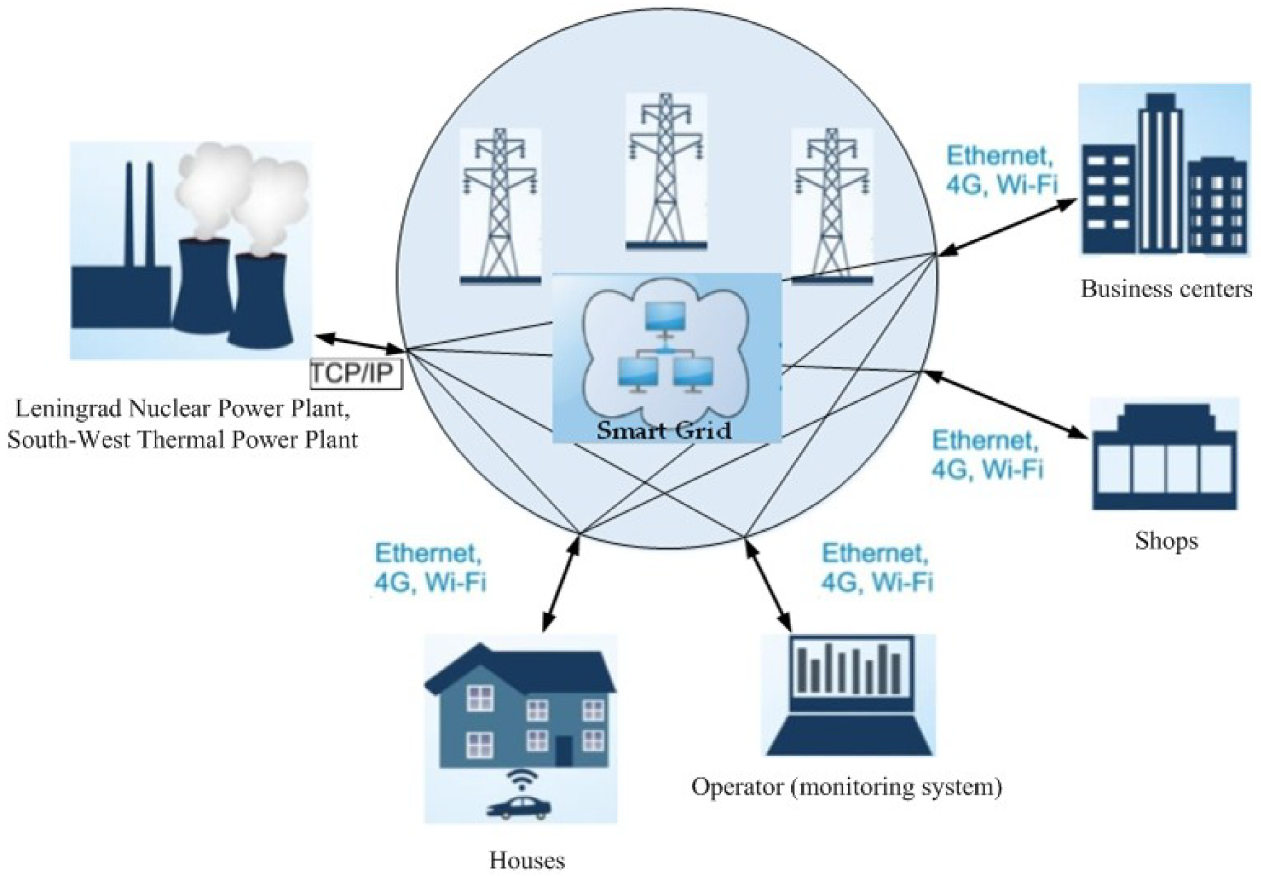
Traffic corresponding to the SG telecommunication network of St. Petersburg (Russia) is chosen as the scenario under study. This network contains 50 high voltage substations, 2200 distribution points and transformer substations, and over 80,000 metering devices (Figure 1). The following technologies are considered as the main technologies for transferring data packets: a family of technologies for packet data transfer between devices for industrial Ethernet networks; mobile communication technologies, allowing data transmission at a speed of 100 Mbit/sec (with mobile subscribers) and 1 Gbit/sec (with stationary subscribers); wireless LAN technology with devices based on IEEE 802.11 standards and Transmission Control Protocol (TCP). In this scenario, the message packet transmission process is stationary. Metering devices are located in houses, shops, and business centers. The source of electricity is the Leningrad Nuclear Power Plant and the South-West Thermal Power Plant. The security control of the SG network is carried out by the operator (monitoring system).

The simulated traffic is a set of data of interest to operators and dispatchers of the SG power system. This data contains the following parameters:

• power factor values;
• power quality parameters within the entire system;
• parameters of the distributed measurement system;
• equipment condition parameters;
• information about places of damage and failures;
• load of transformers and lines;
• profiles and forecasts of electricity consumption and some other parameters.

We consider an SG telecommunication network as a kind of computer network. Therefore, we believe that for the SG telecommunication network, as well as for all computer networks in general, the self-similarity property is valid. This assumption is confirmed by us in the course of experiments.

Considering that the largest amount of information is stored and transmitted to operators and dispatchers of the SG energy system, the monitoring system (operators), as well as the data transmission network of the Leningrad Nuclear Power Plant and the South-West Thermal Power Plant, are chosen as the target of cyber attacks. In the simulation, it is assumed that the edge network equipment has 4 Ethernet ports, each of which has a bandwidth of 1 Gigabit.

In this scenario, the message packet transmission process is stationary. Simulation modeling based on GNS3 software (Galaxy Technologies LLC., Hong Kong, China, https://www.gns3.com/) is used to generate traffic.

The structure of a dataset with normal traffic received using GNS3 software is shown in

Table 1. The structure of a dataset with normal traffic.

	Attribute Name	Comments
1	Flow.ID	A flow identifier (ID) has next format: Source.IP-Destination.IP-Source.Port-Destination.Port-Protocol
2	Source.IP	The source Internet Protocol (IP) address of the flow
3	Source.Port	The source port number
4	Destination.IP	The destination IP address
5	Destination.Port	The destination port number
6	Protocol	The transport layer protocol number identification (i.e., TCP = 6, UDP = 17)
7	Timestamp	The instant of the packet is captured and stored in the next date format: Dd/mm/yyyy HH:MM:SS
8	Flow.Duration	The total duration of the flow
9	Total.Fwd.Packets	The total number of the packets in the forward (Fwd) direction
10	Total.Backward.Packets	The total number of the packets in the backward direction
11	Total.Length.of. Fwd	The total quantity of bytes in the forward direction obtained from all the flow (all the packets transmitted)
12	Total.Length.of. Backward	The total quantity of bytes in the backward direction obtained from all the flow (all the packets transmitted)
13	Packet.Length.Mean	The mean value of the length of the packets registered in the flow (both forward and backward directions)
14	Fwd.Packet. Length.Max	The maximum values in bytes of the packet length in the forward direction
15	Fwd.Packet. Length.Min	The minimum values in bytes of the packet length in the forward direction
16	Fwd.Packet. Length.Mean	The mean value in bytes of the packet length in the forward direction
17	Fwd.Packet. Length.SD	The standard deviation (SD) in bytes of the packet length in the forward direction
18	Bwd.Packet. Length.Max	The maximum values in bytes of the packet length in the backward (Bwd) direction
19	Bwd.Packet. Length.Min	The minimum (Min) values in bytes of the packet length in the backward direction
20	Bwd.Packet. Length.Mean	The mean value in bytes of the packet length in the backward direction
21	Bwd.Packet. Length.SD	The standard deviation in bytes of the packet length in the backward direction

Abbreviations: ID—Identifier, IP—Internet Protocol, TCP—Transmission Control Protocol, UDP—User Datagram Protocol, SD—Standard Deviation.

.

The total number of different Flow.IDs in the dataset is 1,522,917. Eight percent of all records have a Source.IP value of 10.200.7.218 (corresponding to the Leningrad Nuclear Power Plant). Seven percent of all records have a Source.IP value of 10.200.7.217 (corresponding to the South-West Thermal Power Plant). The remaining 85% of the records have other different Source.IP values (there are 3,013,817). Each of the Destination.ID attribute values of 10.200.7.7 and 10.200.7.8 has nine percent of all records. These values correspond to the shops “Passage” and “Gostiny Dvor”. The remaining 82% of records have other different Destination.IP values (their number is 2,939,141).

The time series for self-similarity analysis is formed from the values of the Packet.Length.Mean attribute. The total number of different values for this attribute is 10.7K. The most common values for this attribute are 267.5 and 243.5.

Cyber attacks of the DDoS and “Scanning the network and its vulnerabilities” types are taken into account with the implementation of the attacks. The test equipment for IXIA (Keysight Technologies Inc., Calabasas, California) IP networks is used to generate traffic with this type of DDoS. The Nmap and Xspider software tools are used to simulate the cyber attack “Scanning the network and its vulnerabilities”. When implementing denial-of-service cyberattacks, a distributed network and Synchronize Sequence Numbers Flag (SYN) Flood, Ping Flood, and User Datagram Protocol (UDP) Flood methods are used, while cyber attacks “Scanning the network and its vulnerabilities” are implemented using the probing method. With this method, the security analysis system (for example, Nmap and Xspider) simulates an attack that exploits the vulnerability being checked, i.e., the attack is actively analyzing the vulnerability.

SYN Flood takes undue advantage of the standard way to open TCP connections. When a client wants to open a TCP connection to an open port on the server, it sends an SYN packet. The server receives the packets, processes them, and then sends back an SYN—Acknowledgement Flag (ACK) packet that includes the information about the original client stored in the TCP table. Under normal circumstances, the client sends back an ACK packet, acknowledging the server’s response and, therefore, opening a TCP connection. However, in a potential SYN attack, the attacker sends a whole bunch of connection requests using a spoofed IP address that the target machine treats as valid requests. Subsequently, it processes each of them and tries to open the connection for all these malicious requests. Ping Flood and UDP Flood are implemented by analogy.

For abnormal traffic containing attributes that reflect cyber attacks, additional attributes are included in the dataset structure, shown in

Table 2. Additional attributes, reflecting cyber attacks.

##	Attribute Name	Comments
1	FIN.Flag.Count	The number of times the packets sent in the flaw have the FIN (final) flag bit set as 1. In the normal case, each side terminates its FIN flag.
2	SIN.Flag.Count	The number of times the packets sent in the flaw (in both directions) have the SIN (synchronize) flag bit set as 1.
3	RST.Flag.Count	The number of times the packets sent in the flaw (in both directions) have the RST (reset) flag bit set as 1.
4	ASK.Flag.Count	The number of times the packets sent in the flaw (in both directions) have the ASK (acknowledged) flag bit set as 1.

Abbreviations: FIN—Final Flag, SIN—Synchronize Sequence Numbers Flag, RST—Reset Flag, ASK—Acknowledgment Flag.

.

The values of the FIN, SIN, RST, and ASK flags in the generated dataset depend on the type of cyber attack being modeled. So, for the “Scanning the network and its vulnerabilities” attack, the number of single values for the SIN and ASK flags increases. In traffic prepared for the experiments described in Section 5 below, the proportion of single values for the SIN flag is 20%, and the proportion of single values for the ASK flag is 60%.

Considering the above, the traffic structure, packet header length, flags, checksum, and some others are considered as the main characteristics under study in the dataset.

For the experiment, two datasets are formed. The first dataset includes reference traffic and is used to train the system and analyze traffic without anomalies. The second dataset includes cyber attacks, such as DDoS and “Scanning the network and its vulnerabilities”, and is used to test the effectiveness of the method under consideration and identify its advantages over other methods.

5. Experimental Results

The experiments have served two goals. The first goal is to demonstrate the ability to detect self-similarity in the traffic of the SG network, obtained by simulation. The second goal of the experiments is to demonstrate the possibility of detecting cyber attacks using the proposed method based on the fractal approach.

5.1. Demonstration of the Possibility of Detecting Self-Similarity in the SG Network Traffic

To demonstrate the possibility of detecting self-similarity of traffic in the SG network, we have first modeled and studied several samples containing 1024 points distributed according to the law of fractal Brownian motion with different values of the Hurst exponents: 0.3, 0.5, and 0.8.

Many researchers [23,24,25,26,27] use R/S analysis to find the $H$ parameter for the network traffic. However, the R/S analysis gives a large error, which reaches 20–30% when analyzing non-stationary processes. This indicates the undesirability of its use [28,29,30,31]. Therefore, we have used the DFA method to find the scaling index in non-stationary time series, and DFA and R/S analysis to find $H$ in stationary processes.

It should be noted that when $H$ is changed, the goal is to obtain a random signal as diverse as possible, not similar to the previous one, in order to check the performance of the algorithms as completely as possible, which is necessary to detect various cyber attacks. Therefore, the boundaries of the intervals along the Y-axis are not fixed. The change in $H$ during the simulation is carried out by software. For this, the Matplotlib tool is used. Then, the analysis of the simulated signal self-similarity is carried out using the above algorithms for estimating $H$. The found value of the parameter $H$ is compared with the reference one. Only after testing the algorithms, the transition to the work with real traffic is made.

The first sample is studied with $H=0.8$. Figure 2 shows an example of such a sample. The X-axis represents the sample point numbers. The signal values corresponding to fractal Brownian motion are plotted along the Y-axis.

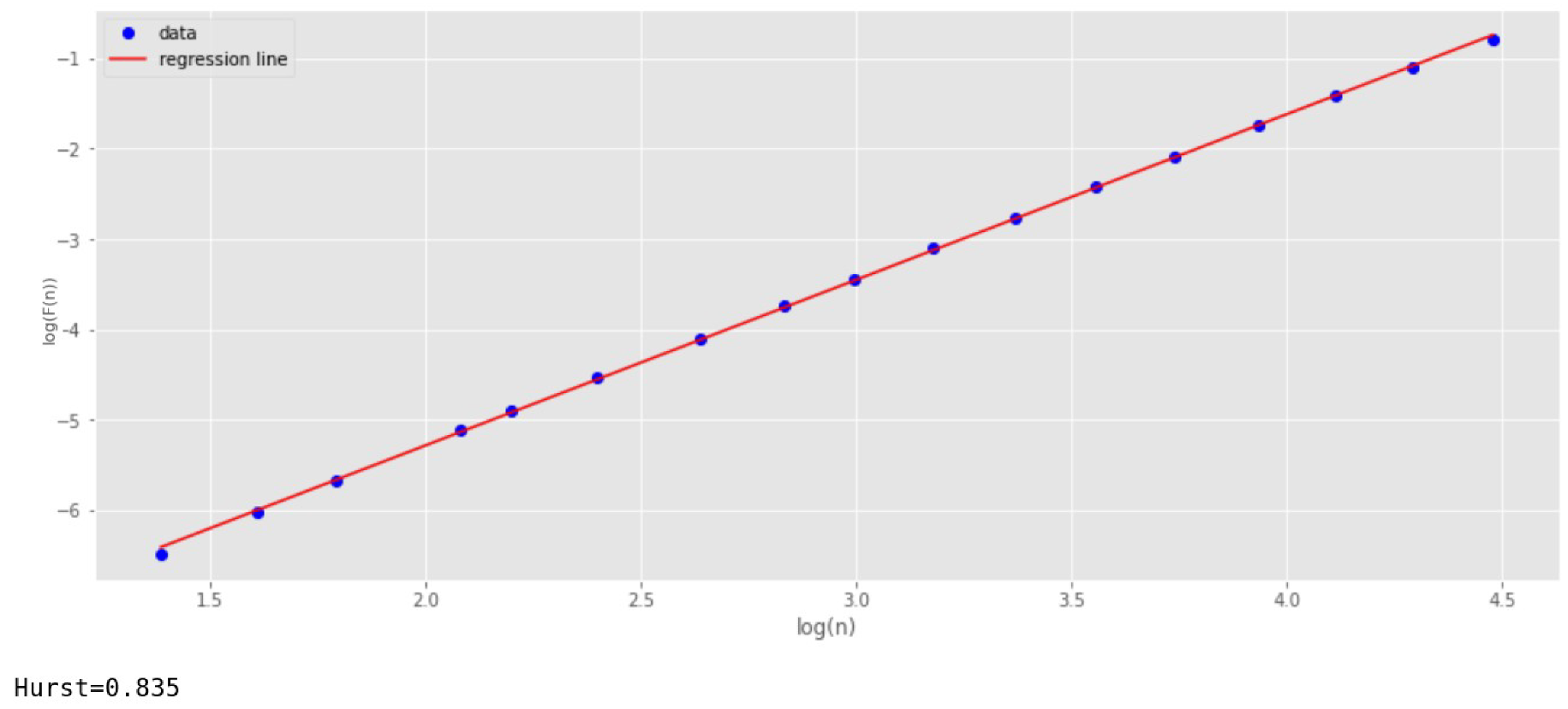
This signal is a non-stationary process that has a long-term memory. Therefore, the DFA algorithm is used to find the $H$ exponent. Figure 3 shows the dependence of the function $\log F\left(n\right)$ (Y-axis) on $\log \left(n\right)$ (X-axis) for this case. To construct the regression line, the least-squares method is used. At the same time, 17 points (scales) are selected along the X-axis. The number of scales is usually chosen at least 10. The larger the number of scales, the higher the accuracy. However, keep in mind that increasing the number of scales enlarges the running time of the algorithm.

The parameter $H$ is determined by the slope of the regression line. For Figure 3, the parameter $H$ shows a value of 0.835. This corresponds to the reference value with a small margin of error.

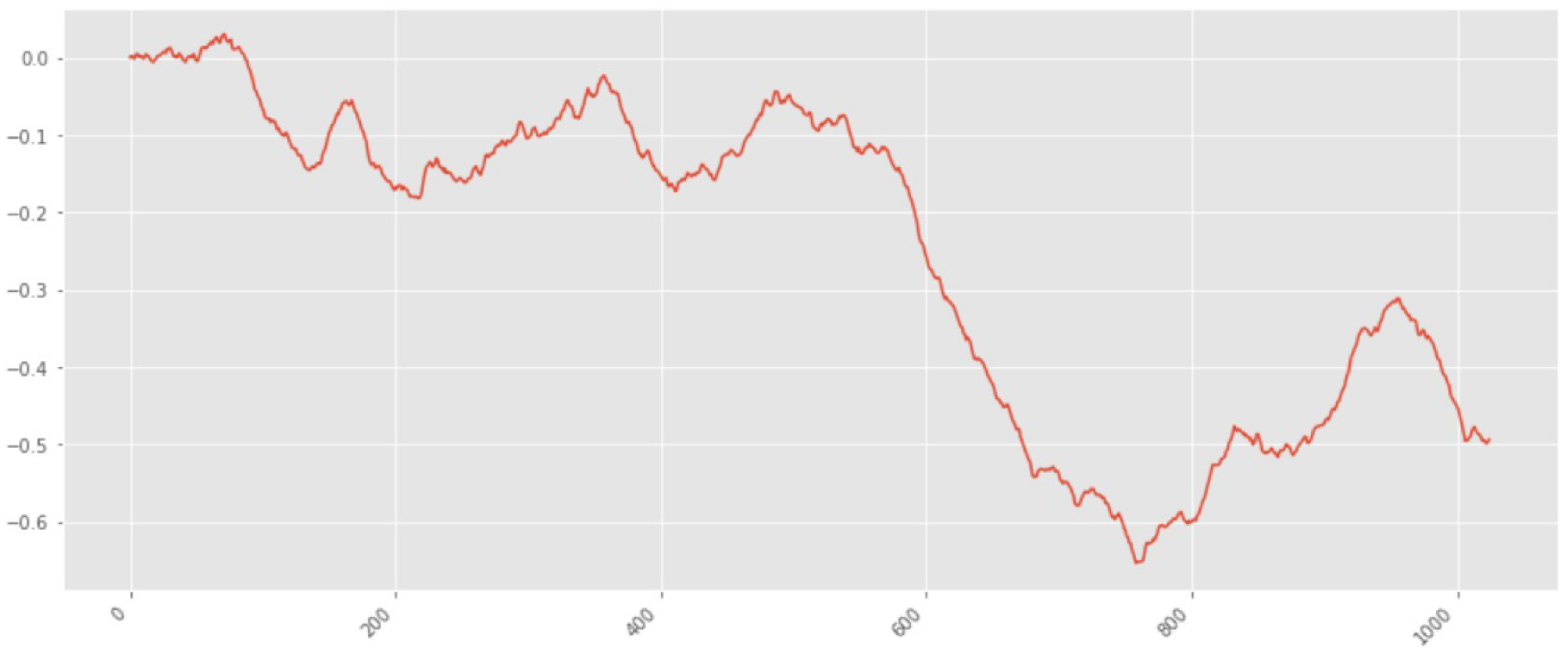
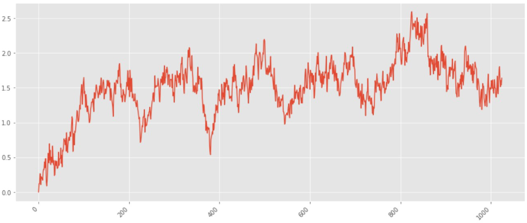
The next study is the value of $H$ equal to 0.3. Fractal Brownian motion, in this case, is shown in Figure 4. It is easy to see that the number of fluctuations in this graph is much larger than for the previous case, and they are stronger in amplitude.

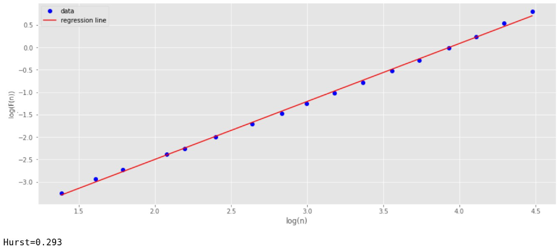
Figure 5 shows the result of calculating $H$ by the DFA method. It is seen that this algorithm has quite accurately determined $H$ as equal to 0.3 (when rounding).

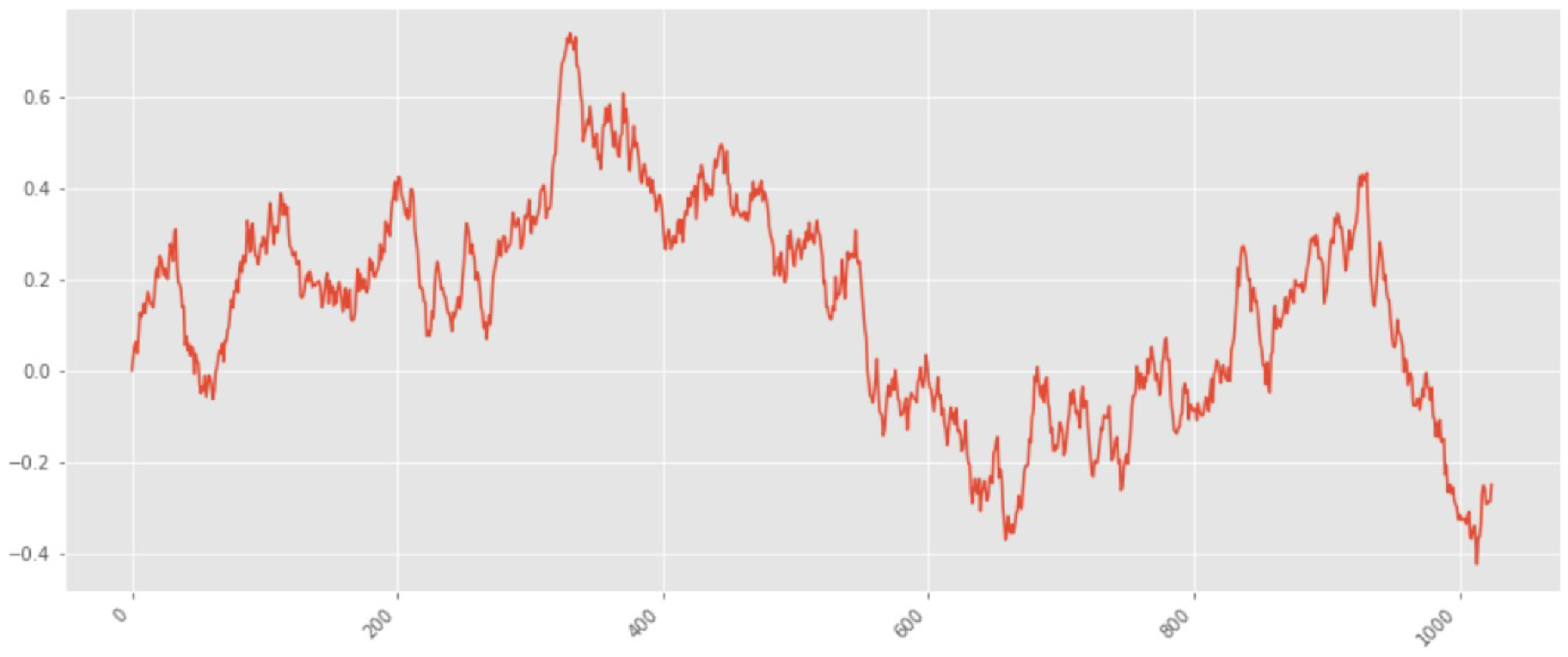
Finally, the DFA algorithm is tested for $H$ of 0.5. This case corresponds to white noise or a chaotic signal (Figure 6).

Using the DFA algorithm, a scaling index of 0.5 is found (Figure 7).

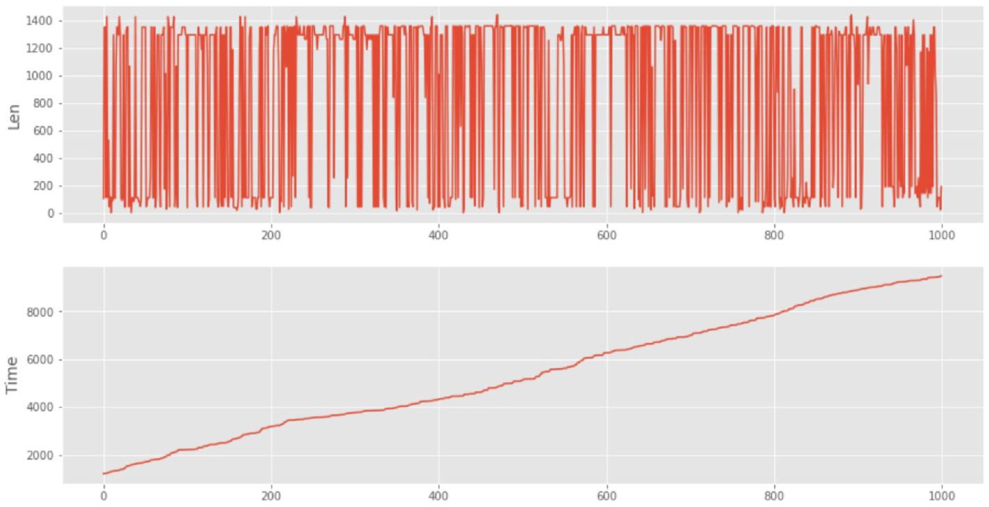
Next, we have studied a reference sample of network traffic for an SG network, containing 1000 TCP and UDP packets. An example of this sample is shown in Figure 8. The sample is simulated using the GNS3 software tool. The sample is represented by two graphs. On the first graph, along the Y-axis, the length of the packet is plotted, and on the second graph, the time of packet arrival is depicted. The X-axis for both graphs is the packet number.

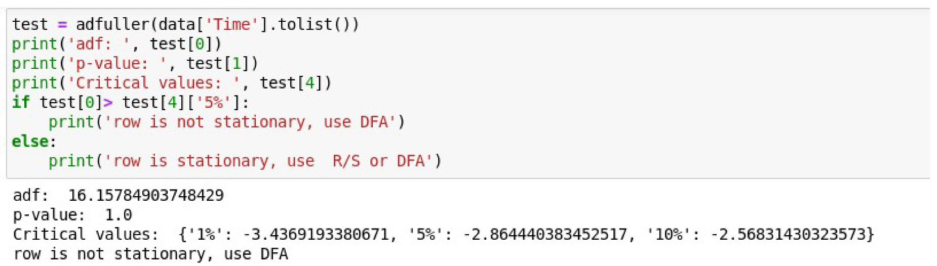
The Augmented Dickey–Fuller test is conducted to confirm the non-stationarity of the time series. Figure 9 shows the result of this test. Listing of the code that implements the check-in the Matplotlib environment and the calculation results are shown.

In Figure 9, the adf parameter denotes a test statistic value. If this value is negative and less than the critical values at 1%, 5%, and 10%, then the null hypothesis in the ADF test is rejected. This will then mean that the series is stationary. In our case, the statistic is 16.15. It is positive and, naturally, greater than the critical values at 1%, 5%, and 10%. This means the null hypothesis is not rejected. The time series, in turn, is not stationary.

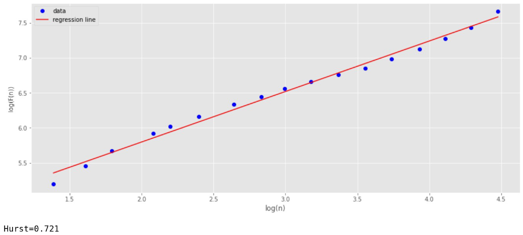
Since the series shown in Figure 8 is non-stationary, we have used the DFA algorithm to analyze the self-similarity property [32,33,34] (Figure 10). This analysis shows the presence in the time series of the self-similarity property with the index $H=1.0$.

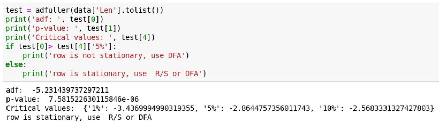
Now, the Augmented Dickey–Fuller test is carried out for a number of network packet lengths, and its stationarity is checked. Figure 11 shows the listing of the code that implements the check and the result of this test.

Figure 11 shows that the test statistic value adf is negative and less than the critical values at 1%, 5%, and 10%.

Therefore, the null hypothesis in the DF test is rejected. This means that a set of network packet lengths is stationary.

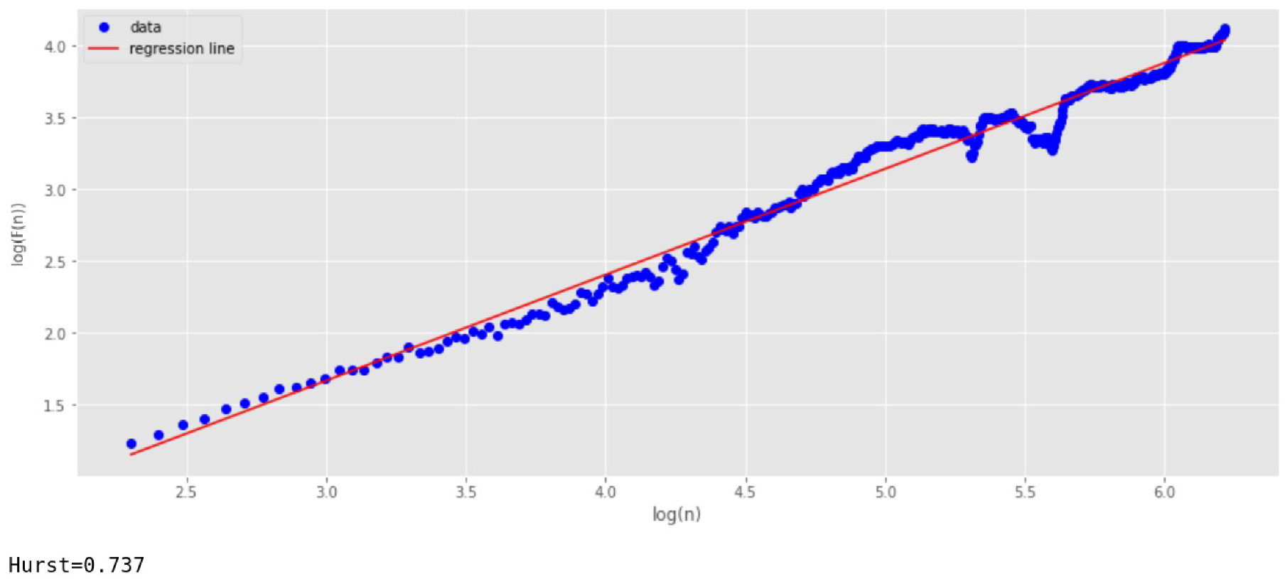
As stated above, several methods can be used to find the scaling index in stationary series: R/S analysis and DFA. We have tested both methods and compared the results obtained (Figure 12 and Figure 13).

To obtain the regression line in the R/S analysis, 100 scales are selected. This is done in order to improve the accuracy of determining the indicator $H$. As can be seen from Figure 12 and Figure 13, both methods give approximately the same result.

Thus, the experiments carried out on the reference samples, in which there are no anomalies caused by the impact of cyber attacks, have demonstrated the presence of self-similarity of the SG network traffic and the possibility of a sufficiently accurate determination of the self-similarity index based on the proposed approach.

5.2. Detecting Anomalies and Cyberattacks in the SG Network Traffic

To find anomalies in the SG network caused by cyber attacks, the traffic is first divided into groups, and the Hurst exponent is found for each of the groups. The analysis shows that the larger the number of groups, the earlier anomalies (cyber attacks) can be detected, and actions need to be taken to eliminate (prevent) them. However, as the number of groups increases, the number of points from which values are calculated decreases, which may affect the measurement accuracy. Therefore, experiments are carried out to find the minimum acceptable size of such a group.

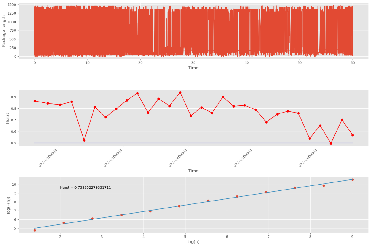
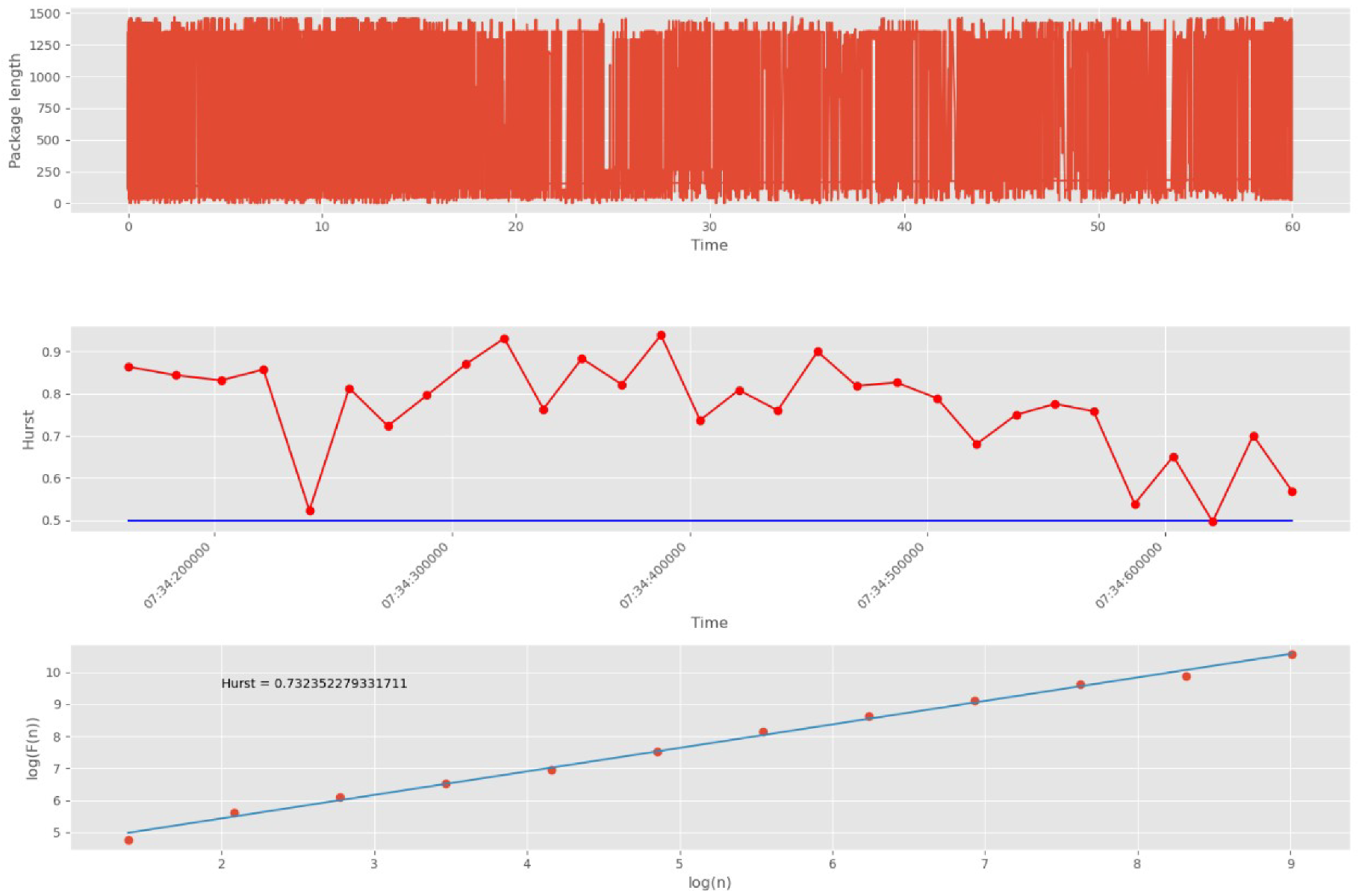
Initially, 10,000 network packets are split into 30 groups. Figure 14 shows DataFrame UDP traffic, its division into groups of packets, and an estimate of the Hurst exponent for each group, as well as an estimate of the self-similarity of all traffic without dividing it into groups.

The blue straight line in the second graph indicates the threshold corresponding to the white noise boundary ($H=0.5$). The points on the second graph correspond to the packet group numbers (30 points in total). The points on the third graph correspond to scales (12 points in total).

As noted above, the number of scales affects the accuracy and duration of the algorithm. The larger the number of scales, the higher the accuracy, and, conversely, the shorter the duration of its work. Since in the proposed approach, the factor of the rate of detection of anomalies caused by cyber attacks is of higher importance than the accuracy of calculating the self-similarity index, we have decided to limit ourselves to a small number of scales equal to 12.

As can be seen from Figure 14, the measure of fractality for all groups of packets lies entirely above the 0.5 mark. This indicates the presence of self-similar properties in each group. In addition, the third plot (logarithmic regression line) shows the Hurst parameter for the entire DataFrame, which confirms the presence of fractal properties and repetitive processes.

Next, we have tested abnormal network traffic dumped during the DDoS attack and the “Scanning the network and its vulnerabilities” attack. The aim is to select the maximum number of partition groups, at which the estimated parameter $H$ will be calculated with high accuracy.

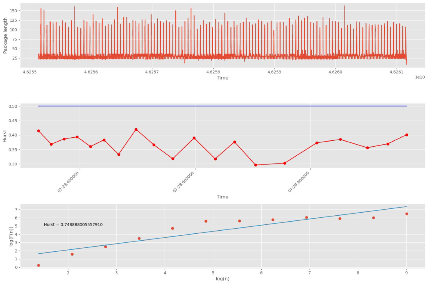
Initially, 20 groups of 500 packets each are selected (Figure 15).

As can be seen from Figure 15, the values of all Hurst exponents at sites of 20 groups are below 0.5. This indicates a violation of the fractal structure of traffic and the presence of anomalies in it. In addition, the series under study shows non-stationary properties. Therefore, the proposed approach is able to detect anomalies in intervals (groups) of 500 network packets.

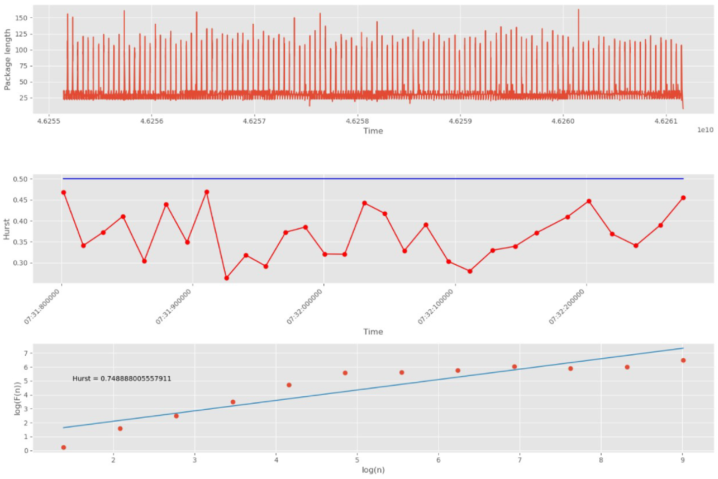
Shortening the time interval by increasing the number of groups to 30 is tried (Figure 16).

Figure 16 shows that splitting into 30 groups does not reduce the accuracy of the algorithm.

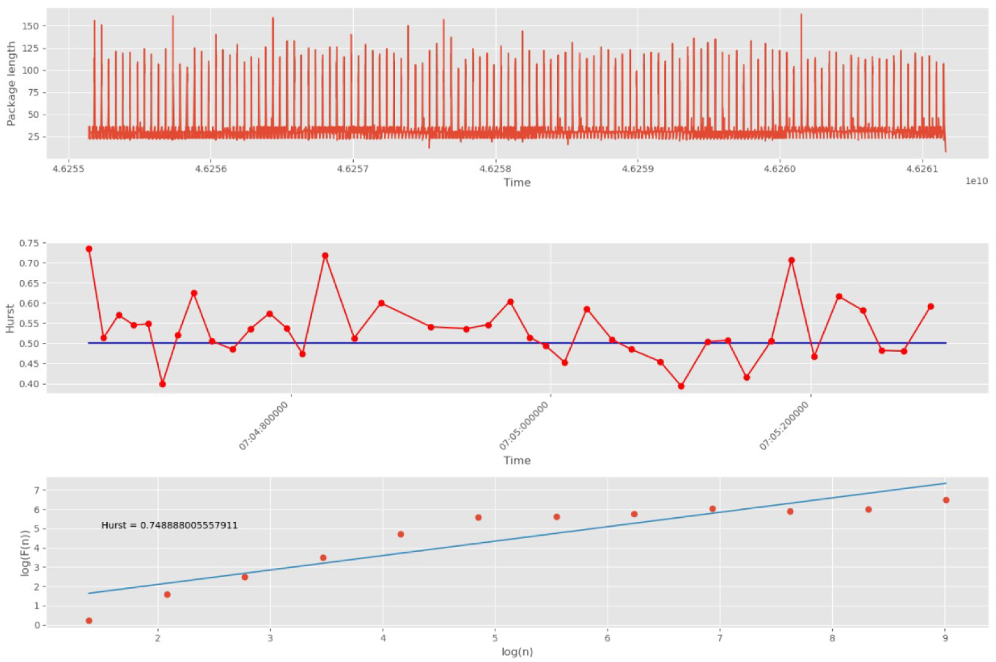
When analyzing the division into 40 groups, each of which consists of 250 network packets, one can already see the manifestation of self-similarity properties on some of them (Figure 17).

On the one hand, this may indicate the absence of anomalies in the investigated interval. On the other hand, this behavior indicates deterioration in accuracy due to a small sample. Therefore, such a partition is unacceptable. The previous partition should be considered as the sought one, i.e., division into 30 groups.

5.3. Comparative Assessment with Other Approaches and Methods for Detecting Cyber Attacks

A comparative assessment of the effectiveness of the method under consideration is carried out on the basis of its comparison with other known methods for detecting computer attacks, such as signature-based methods, statistical methods, and machine learning methods. The results of this comparison are presented in

Table 3. Results of a comparative assessment of the known methods of detecting cyber attacks.

Method Name	Detection Rate	Detection Accuracy		Traffic Type		No False Detection
		For Known Attacks	For Unknown Attacks	Stationary	Non-Stationary
Signature-based	High	High	Low	High	Low	Middle
Statistical	Middle	Middle	Middle	High	Low	Middle
Machine learning	Middle	High	Middle	High	Low	High
Fractal analysis	High	Middle	Middle	High	High	Middle

. For comparison, a three-point scale is used—“High”, “Middle”, and “Low”.

The main considered parameters of the compared methods are the speed (rate) and accuracy of detecting cyberattacks, both known and unknown, the ability to work with stationary and non-stationary traffic, as well as the frequency of false positives.

Signature-based methods use predefined rules [35]. Therefore, they are fast enough and have high accuracy in detecting known types of cyber attacks. However, they are unable to detect new, unknown types of attacks, including targeted attacks. In addition, they have average indicators of no false detection.

Statistical methods [36,37] use accumulated statistics. For this reason, they are inferior to signature-based methods in terms of detection rate and detection accuracy of known attacks. At the same time, in some cases, they are able to detect unknown attacks. For no false detection, they have the same capabilities as signature-based methods.

Machine learning methods are currently quite diverse and well developed [38,39,40]. Considering that in these methods, the process of attack detection is necessarily preceded by the training process on the control sample, we believe that these methods are inferior to signature-based methods in terms of the attack detection rate. However, these methods have higher detection accuracy for known attacks and good detection accuracy for unknown attacks. At the same time, the proportion of false positives in machine learning methods is low.

The proposed fractal analysis method has a high detection rate comparable to signature-based methods. This is achieved by splitting the original traffic into groups of packets of appropriate sizes. A decision on the presence of an anomaly in traffic is made immediately after a self-similarity violation is detected for the first such group. However, since anomalies can be caused by various reasons, not only related to cyber attacks, it should be considered that the detection accuracy of known and unknown attacks, as well as false positives, is average. At the same time, the undoubted advantage of the proposed approach is the possibility of its application not only for stationary traffic but also for non-stationary traffic. Other methods for non-stationary traffic either do not work or have very low efficiency.

Thus, an analysis of the results of a comparative assessment shows that one of the main advantages of fractal analysis is the speed of its operation, as well as the ability to detect both known and unknown cyber attacks for any type of traffic.

Only an increase in the number of processed parameters of the data transfer protocol header (packet length, flags, etc.) leads to an increase in the calculation time.

5.4. Discussion

The results of experiments show, first of all, that the SG network traffic has fractal properties, that is, it has the property of self-similarity on large volumes of traffic.

In addition, the experiments demonstrate that the proposed approach to assessing the self-similarity of the parameters of the system’s functioning using fractal indicators has fairly high efficiency.

The main advantage of this approach is the high speed of detection of anomalies caused by cyber attacks. The determination of the Hurst coefficient is performed in a few microseconds, depending on the performance of the computer equipment.

Other advantages of this approach include a fairly high accuracy in detecting anomalies, as well as low demands on system resources. In addition, the proposed approach is universal due to the presentation of processes in the form of time series. The type of information transfer protocol such as UDP, TCP, or Internet Control Message Protocol (ICMP), as well as the type of information transmitted (service information, synchronization, useful information), does not affect in any way the time for determining the Hurst coefficient. It is invariant to the types of destructive influences and does not require tuning or adaptation to the detection of specific types of attacks, including those previously unknown.

It should be noted that R/S analysis is only suitable for stationary processes and is inferior to DFA in terms of computation speed and detection accuracy. Only an increase in the processed parameters of the data transfer protocol header (packet length, flags, etc.) leads to a change in the calculation time. In addition, if the traffic is not stationary, i.e., the transmission of message packets in SG is not uniform in time, the accuracy of detecting anomalies in traffic is slightly reduced.

However, despite the above-listed advantages, this method is not a panacea because it does not give an exact indication of a specific abnormal packet, but characterizes the totality of packets as a whole. This condition does not allow using this method to detect anomalies in real-time but brings it closer to this due to its ability to focus on processing small sample groups. In other words, the proposed approach should be used firstly to quickly detect the presence of anomalies in the traffic with the aim of further using other methods of cyber attack detection (signature-based methods or machine learning methods) in order to improve the accuracy of their detection and reduce the likelihood of false positives. In other words, it can launch other methods of cyber attack detection.

In addition, it should be noted that the studies conducted so far only demonstrate the potential and effectiveness of the proposed approach for cyber attack detection in the SG network. The practical implementation and further improvement of this method, its extension to various types of cyber attacks, as well as its interaction in the security system with other methods determine further areas of research.

6. Conclusions

The paper has proposed a new approach to the detection of cyberattacks in the SG network, based on the fractal analysis of network traffic. The proposed approach is based on the application of the main provisions of the theory of fractals and the use of methods for assessing self-similarity proposed by this theory, such as the extended Dickey–Fuller test, R/S analysis, and the DFA method. When testing fractal methods that allow researching long-term dependencies in the traffic of the SG network, the DFA method has turned out to be more effective than R/S analysis due to its ability to process not only stationary but also non-stationary series with high accuracy. For SG networks, the advantage of DFA over the older R/S method is that it removes local trends through least squares regression fit and is relatively immune to non-stationarity. Therefore, DFA allows the detection of long-range correlations embedded in non-stationary series, which is quite typical for SG networks, avoiding false detection of explicit long-distance correlations that are non-stationary artifacts.

Based on the results of experimental verification, we can conclude that the proposed approach is quite correct. Experiments have shown that there is a characteristic time after which the Hurst exponent changes sharply. This time indicates the amount of system memory. Experimental results also indicate that self-similar properties are inherent in any network traffic. When network anomalies appear, caused, for example, by cyber attacks, such as DDoS and “Scanning the network and its vulnerabilities,” the nature of these properties begins to differ significantly from normal traffic.

Further research is related to the integration and combination of the proposed approach with known methods for detecting network traffic anomalies.