Abstract
Integration of Information and Communication Technology (ICT) in modern smart grids (SGs) offers many advantages including the use of renewables and an effective way to protect, control and monitor the energy transmission and distribution. To reach an optimal operation of future energy systems, availability, integrity and confidentiality of data should be guaranteed. Research on the cyber-physical security of electrical substations based on IEC 61850 is still at an early stage. In the present work, we first model the network traffic data in electrical substations, then, we present a statistical Anomaly Detection (AD) method to detect Denial of Service (DoS) attacks against the Generic Object Oriented Substation Event (GOOSE) network communication. According to interpretations on the self-similarity and the Long-Range Dependency (LRD) of the data, an Auto-Regressive Fractionally Integrated Moving Average (ARFIMA) model was shown to describe well the GOOSE communication in the substation process network. Based on this ARFIMA-model and in view of cyber-physical security, an effective model-based AD method is developed and analyzed. Two variants of the statistical AD considering statistical hypothesis testing based on the Generalized Likelihood Ratio Test (GLRT) and the cumulative sum (CUSUM) are presented to detect flooding attacks that might affect the availability of the data. Our work presents a novel AD method, with two different variants, tailored to the specific features of the GOOSE traffic in IEC 61850 substations. The statistical AD is capable of detecting anomalies at unknown change times under the realistic assumption of unknown model parameters. The performance of both variants of the AD method is validated and assessed using data collected from a simulation case study. We perform several Monte-Carlo simulations under different noise variances. The detection delay is provided for each detector and it represents the number of discrete time samples after which an anomaly is detected. In fact, our statistical AD method with both variants (CUSUM and GLRT) has around half the false positive rate and a smaller detection delay when compared with two of the closest works found in the literature. Our AD approach based on the GLRT detector has the smallest false positive rate among all considered approaches. Whereas, our AD approach based on the CUSUM test has the lowest false negative rate thus the best detection rate. Depending on the requirements as well as the costs of false alarms or missed anomalies, both variants of our statistical detection method can be used and are further analyzed using composite detection metrics.
1. Introduction
The integration of Information and Communication Technology (ICT) in the control, protection and monitoring of power systems can offer several advantages with respect to the efficiency of the production, transmission and distribution operations. Combining intelligent components with a well-designed Substation Communication Network (SCN) according to specific norms and recommendations shall ensure an optimal operation of the power systems with a significant economic efficiency. However, a major drawback of the increased ICT interconnection is the larger exposure to malicious cyber-attacks.
Research in this field (e.g., [1,2,3]) has shown the different vulnerabilities of Smart Grids (SGs). In order to secure modern power systems, several aspects shall be considered including a reliable and safe software for control systems [4] and a secure communication network in the power grid. Electrical substations, in particular, might be subject to several vulnerabilities [2]. For instance, a modern electrical substation in Ukraine was the target of an attack that is considered to be the biggest threat to Industrial Control System (ICS) after the infamous Stuxnet [5].
In order to secure the communication network in electrical substations, several aspects shall be considered. From an information security perspective, confidentiality, integrity and availability of the data transmitted within the substation network shall be tackled. Confidentiality uses techniques such as access control to ensure the protection of the data against unauthorized access, disclosure or theft. Data integrity refers to protecting the data against any improper modification or alteration to guarantee its accuracy and consistency. Mechanisms to ensure the integrity of the data within ICS or SCN shall account for the strict Real-Time (RT) requirements expected in such environments. Authentication methods adapted for those particular conditions have been developed in literature [6,7,8]. Ensuring the availability of data in SGs is considered to be the most critical requirement in power systems [9]. Attacks against SGs might exploit security vulnerabilities to attempt to deny legitimate communications within the network traffic that would result in blocking legitimate information and services. Additionally to the availability of the data, the real-time reliability of the communication networks in ICS [10] and in electrical substations is necessary to guarantee an optimal operation of the grid.
In order to tackle threats such as Denial of Service (DoS) or flooding attacks that might hinder the availability of the data within the SCN, Intrusion Detection System (IDS) can be adopted. Choosing a well-adapted IDS relies on several factors among which an adequate knowledge of the characteristics of the network traffic can be of a great relevance. The focus on the physical process as well as the use of several protocols among ICS increases the complexity of studying the network traffic behavior.
We present the study of the network traffic within electrical substations based on the International Electrotechnical Commission (IEC) 61850 standard. First, we analyze the different statistical network features. A better understanding of the characteristics of the SCN helps us define a well-adapted mathematical model to describe the network traffic in electrical substations. Second, we define an Auto-Regressive Fractionally Integrated Moving Average (ARFIMA) model that can accurately account for the Short-Range Dependency (SRD) as well as the Long-Range Dependency (LRD) in the network traffic data as shown by the reported results. Deriving a mathematical representation of the network traffic data in IEC 61850 substations can considerably support the design of the network architecture of future electrical substations as well as the overall performance of the network communication. Then, we underline the knowledge about the behavior of the SCN and develop two techniques for a model-based Anomaly Detection (AD). The proposed approaches are based on statistical hypothesis testing using the Generalized Likelihood Ratio Test (GLRT) to detect anomalies resulting from changes in the traffic patterns such as flooding attacks. The AD problem as defined in our approach can be formulated as a change point detection problem. Statistical detection methods have been used in general for the previously mentioned problem, considering their high reliability [11]. The novelty of our work resides in adapting those methods to enhance the availability of the network traffic data in electrical substations and thus their overall cyber-physical security. Our AD technique is able to detect multiple anomalies at unknown change times while assuming unknown noise parameters. We select carefully specific detectors for the hypothesis testing to suit the characteristics and the requirements of IEC 61850 electrical substations. Our experiments to test the performance of the model-based AD approach, with both variants, show strong results in terms of detection accuracy and minimizing False Alarm (FA) rate and detection time. The main contribution of our work is to adapt two well-known detectors, GLRT and CUSUM, to present a structured method for the detection of DoS attacks in IEC 61850 electrical substations. The overall detection performance of the new statistical AD method outperforms available approaches as explained in Section 6.3.
The detailed contributions of this work are as follows:
- We conduct a structured analysis of the GOOSE network traffic in a SCN from a simulation case study that can be further applied to a network traffic from a real substation
- We model the GOOSE communication in an IEC 61850 substation using an ARFIMA model including the parameter estimation and the model prediction. We evaluate the accuracy of the suggested model using well-established criteria from the data-driven modeling field.
- We present a structured AD method based on two different approaches to detect flooding attacks using two well-known statistical tests while assuming an unknown change time and unknown model parameters under each hypothesis
- We evaluate the performance of the AD method with both detectors, in terms of basic and composite detection metrics, using a simulation case study under different rates of SNR.
The remainder of this work is organized as follows: an overview of the different intrusion detection techniques in power systems with a particular focus on the AD approaches is provided in Section 2. In Section 3, we analyze the characteristics of the process network traffic. The derived characteristics help us select an appropriate regression model, in this case an ARFIMA model to describe the data. Thus, we present the ARFIMA modeling of the process traffic in IEC 61850 Substations in Section 4. Conclusions about the mathematical modeling of the SCN traffic data lead us to develop two detection schemes based on statistical hypothesis test as discussed in Section 5. Section 6 mainly focuses on the evaluation of the selected ARFIMA model as well as the detection approaches using an adequate use case. In Section 7, we present the conclusions of our work.
2. Intrusion Detection Systems (IDSs) in Energy Systems
There has been extensive work in literature ([12,13,14,15,16]) aiming at detecting anomalies in ICS and Supervisory Control And Data Acquisition (SCADA) systems. In the present paper, we will focus on efforts to develop IDSs in a particular application field which is energy systems. There are several possible ways to classify IDSs. A commonly used one is based on the ability of the IDS to detect, the so-called, zero-day attacks.
2.1. Signature-Based Approaches
The first category is known as signature-based IDS and its working principle consists mainly of collecting attack patterns into a database. Comparison between gathered data and collected attack signatures allows the detection of anomalies. This type of method is very efficient in detecting anomalies with no False Alarms (FAs) under the condition that meaningful signatures are defined. Work developed by Premaratne et al. [13] is one of the pioneer studies on IDS in electrical substations. Their method is based on a Snort rule-based IDS for Intelligent Electronic Devices (IEDs) in IEC 61850 substations. The blacklisting relies on rules established using an experimental setup to simulate attacks.
Analysis of Modbus/TCP traffic using Quickdraw tool to identify anomalies was proposed in [14]. Quickdraw is a preprocessor of Snort developed by Digital Bond. Several rules including specifications for Modbus/TCP, DNP3 and Ether/IP protocols are proposed. A framework for dynamic rules generation and Deep Packet Inspection (DPI) that can be applicable for Snort and Suricata was developed by Niventhan and Papa [17].
Signature-based IDS have typically two main drawbacks. First, the challenges related to the creation of a relevant set of rules that need to be regularly updated and maintained. Second, signature-based IDS are only able to detect known attacks. When considering the scarcity of attack databases in ICSs and SCADA systems due to the sensitivity of the data, signature-based IDS might not be an optimal choice for securing the network traffic also within power systems.
2.2. Anomaly Detection (AD) Approaches
Another category of IDSs is anomaly-based detection. The AD methods are based on characterizing the normal behavior of a system. It is thus assumed that any abnormality or deviation from the normal behavior is considered as an anomaly. The main advantage of this technique is the ability to detect unknown attacks. Thus, AD methods in SCADA and ICSs have been extensively used over the past few years: indeed, model-based detection is commonly used in conventional IDSs and can be particularly relevant for monitoring unknown attacks in SCADA systems [12]. Similar assumption about the periodicity of the network traffic in ICS was demonstrated by Barbosa et al. [18] and further used to propose an AD tool. The proposed tool, PeriodAnalyser, whitelists the traffic including Modbus/TCP and Manufacturing Message Specification (MMS) protocols according to a learned model.
Other anomaly-based IDSs were based on communication patterns to detect anomalies. Some AD methods use Machine-Learning (ML) techniques to model communication patterns such as One-Class Support Vector Machine (OC-SVM) [19]. Shang et al. [20] use OC-SVM to model normal communication that is based on computing a hyperplane in the feature space to distinguish between normal and anomalous objects. The considered communication includes only Modbus/TCP static exchanges between a client and a server. The previously mentioned work is telemetry-oriented and is based on the assumption of periodicity of the network traffic which is not always the case of MMS messages, for instance. Another limitation is the absence of any semantics in the detected anomalous packets with little to no insight on the cause of the traffic behavior.
Several AD methods that are based on statistical techniques have been used in the literature. The network traffic may exhibit several statistical properties that can be analyzed in order to detect intrusions or attacks. Statistical approaches are commonly used for change point detection and thus for AD. To detect anomalies in IEC 61850 automation systems, Kwon et al. [21] use network telemetry metrics and protocol specifications. Metrics considered for Generic Object Oriented Substation Event (GOOSE) AD are GOOSE message frequency, counter of received GOOSE messages and timestamp of most recent GOOSE messages. Whereas for MMS, features are limited to the command type. Testing and evaluation of the method are performed using a dataset of network traffic from a Korean SG testbed. In the presented model, only periodic GOOSE traffic are considered while omitting legitimate fault events. Thus, the proposed AD is only based on the mean and the standard deviation in network metrics which assumes that the network traffic can be simply modeled as a signal embedded in White Gaussian Noise (WGN). Such hypothesis does not apply to the network traffic in electrical substations as demonstrated in the present work.
2.3. Hybrid Approaches
To overcome limitations of signature-based approaches and AD systems, an increasing number of IDSs adopt a hybrid approach to detect anomalies using signatures and anomaly detection. A three-level IDS was developed by Cheung et al. [12]. The two first levels consider checking the protocol specifications for Modbus/TCP and network segmentation and access policies, and they are rule-based. The rules were implemented in the open-source IDS software Snort. The third level was learning-based. The authors in [15] implemented a DNP3 parser that was integrated to the open-source network analyzer Zeek (previously Bro). A set of rules to check the packets structure as well as the semantics was developed. To identify malicious commands, the state estimation of the simulated system was predicted and results were integrated with the overall IDS. Some other works [22,23] integrate also Zeek for detection of intrusions in SCADA systems. In a similar approach to Cheung et al. [12], Yang et al. [24] proposed IDS specifically designed for IEC 61850 electrical substations that is further extended to a multidimensional IDS [16]. A four-layer model was presented including access control detection, protocol whitelisting, model-based detection for station and process bus and a multiparameter based detection. Specific input features for GOOSE and Sampled Values (SV) protocols were used in the IDS based on the standard definitions and the configuration system files. Other telemetry-based characteristics were learned from the traffic including packet transfer rate per second, transfer byte size per second, length and size of the packets. A simple thresholding procedure was used to detect if any of the captured traffic characteristics is beyond a minimum and a maximum value.
Few of the previously mentioned works take into account the specific characteristics of electrical substations based on IEC 61850. We present an adequate statistical method based on a well-defined statistical hypothesis testing for the detection of flooding attacks which combines a good detection performance of ML methods with the robustness of statistical approaches [11].
3. Characteristics of the Process Network Traffic
Adaption of recommendations in the IEC 61850 standard allows the use of advanced technologies including IEDs, standardized protocols, a systematic object-oriented structure for the configuration of the Substation Automation System, Ethernet-based communication and possibility of remote control actions.
Typical IEC 61850 substation models have a hierarchical structure with three different levels, namely the station, bay and process layers. The station level includes engineering workstations, Human-Machine Interfaces (HMIs) and gateways to the Energy Management System (EMS) and SCADA systems in order to monitor and regulate the generation, transmission and distribution of the power to the consumers. IEDs from the bay level are mainly responsible for the protection and control operations within the substation. They communicate with each other and with the station level via a station bus using MMS and GOOSE protocols.
Voltage and current signals are transmitted from power equipment to the process level through Merging Units (MUs) and relays that control for instance the tripping of CBs. GOOSE and SV protocols are used between the process and the bay levels to multicast digital voltage and current signals from Current Transformers (CTs) and Voltage Transformers (VTs). The process level network is Ethernet switch-based fiber-optic network. An Ethernet switch is also used for the station bus.
The use of different protocols throughout the SCN results in an increased challenge of understanding the network communication patterns. In the present work, we will mainly focus on the process level network. There are different types of messages exchanged within the substation and are divided into three types from a data flow perspective [25]. Cyclic data flows are time-driven data that are commonly used for transmitting power measurements from field devices.
For instance, SV messages, that are generated from MUs and transmitted to P&C IEDs in the bay level, result in cyclic data flows. This communication carries time-critical information and contains large amounts of data. When a fault occurs, GOOSE messages change from a cyclic mode to a burst mode. Burst data transmit information about protection actions and changing status of CBs. In fact, the process network layer has unique characteristics as it includes large multicast traffic that is periodic in general but which includes bursty sequences. Such features can be challenging to analyze using traditional models.
Thus, a first step for us is to analyze the process traffic. We underline a set of relevant characteristics that is established based on [26]. Floyd and Paxson introduce a method to “search for invariants” to tackle the difficulties in modeling Internet traffic [26]. The term invariant is used to refer to a behavior that was empirically proven to hold in a very wide range of environments. In this work, we consider three invariants in order to characterize the process traffic.
3.1. Diurnal Patterns
One of the properties that can be observed in the network traffic is the variation in the activity, for instance, according to specific times. This dependency is not only related to human activity but also to network protocols, especially those used in the industrial field [26]. Observations of the number of active connections, packets per second and bytes per second might reveal diurnal patterns in the network activity. To conclude the presence of diurnal patterns, a relatively large dataset of several days or weeks shall be available.
3.2. Distributional Considerations of the Data
The data flow for the SCN traffic was characterized by several models depending on the type of the transmitted messages. According to the transmitted information between different components of an electrical substation, seven types of messages are defined in IEC 61850 to transmit different types of information such as the protection commands or the measurement values from physical devices [27]. Fast or medium speed messages have different characteristics from, for instance, file transfer function or access control command messages. Thus, they can be divided into three different categories based on their data flow characteristics, namely, cyclic, stochastic and burst data [25]. A Pareto distribution for burst data flow was suggested in [25], whereas in [7], a Weibull distribution was used instead as it is claimed to fit better increasing retransmission scheme of bursty GOOSE messages. Network in general Internet traffic can be characterized by heavy-tail distributions such as Ethernet bursts [28] and FTP activity.
Modeling the network traffic in electrical substations is a challenging task due to the different operation modes including normal operation and burst data in case of faults. Studies focusing on describing the network traffic ([29,30,31]) show that the GOOSE network traffic exhibits short-range dependency, self-similarity and LRD features. Some research works have been conducted to model the substation communication network. However, few of them consider the self-similarity of the network traffic such as [29,30]. In the next section, we will study the possible presence of self-similarity features in the GOOSE network traffic data.
3.3. Self-Similarity
The self-similarity can be seen in practice by the presence of extended periods where the traffic is larger than the sample mean at different time scales. The degree of self-similarity in the network traffic is commonly determined using the Hurst parameter [32].
These periods of “spikes” in the traffic are referred to as “burstiness” [33]. Let be a time-series of size N. If the time-series is self-similar, the following holds
where is an equality in the sense of finite dimensional distribution, H is the Hurst parameter and is the aggregated sequence by m of x:
Several tests have been commonly used in literature ([26,33]) to show self-similarity of the data. Two of the most known visual methods to show self-similarity are the R/S analysis and the variance-time plot [34].
For the next description of both tests, let be the throughput at time k with N being the size of the time series.
3.3.1. Variance-Time Plots
The first test to verify the self-similarity of a time- series is the variance-time plot. The presence of self-similarity can be checked by observing the variance function of defined in Equation (2) versus the aggregation level m.
The variance of the aggregated process defined in Equation (2) is calculated as follows:
The variance plot, depicted in Figure 1, is defined by plotting the variance of the aggregated process , versus different aggregation levels in log-log scale.
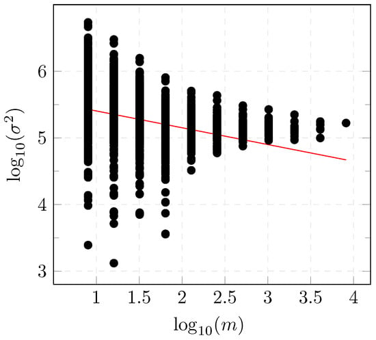
Figure 1.
Variance-time diagram.
The Hurst parameter H can be obtained from the previous plot with a line fitted to the curve using least-squares with the relation which gives a value of for the dataset presented in Section 6.1.
3.3.2. Rescaled Adjusted Range R/S
The R/S method is based on first dividing the time-series into nonoverlapping intervals of length l. The partial sum for each of the intervals is then calculated. Let or be the sample mean of the time series with starting point and size L,
and be the sample standard deviation of a the time series with starting point and end point
The partial sum is defined as follows:
with u being a running index of k within the interval .
The rescaled adjusted range (R/S) statistic is defined as the quotient of the difference between the maximum and the minimum of the partial sum and the standard deviation of the considered time series and is calculated as follows [35]:
Figure 2 represents the versus for the considered dataset. The slope of the regression with the least-squares method of versus represents the estimate of the Hurst parameter which is equal to for the dataset described in Section 6.1.
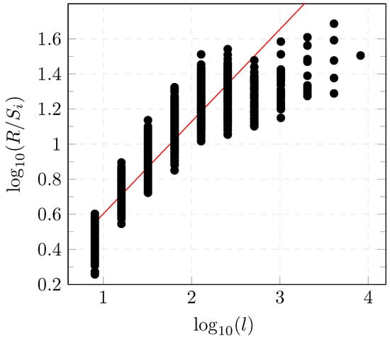
Figure 2.
R/S diagram.
According to both tests, results show that the estimate of the Hurst parameter of the considered dataset lies between and 1 which indicates the self-similarity of the considered process. The time series representing the GOOSE network traffic in electrical substation has a statistical LRD between the current value and values in different times of the series. One of the commonly used models to describe long-memory characteristics is the ARFIMA model [36].
4. ARFIMA Modeling of the Process Traffic in IEC 61850 Substations
After discussing the unique features of the IEC 61850 GOOSE traffic, we select an Auto-Regressive Fractionally Integrated Moving Average (ARFIMA) model to describe the network traffic. In the following, we present explanations of concepts necessary to describe a suitable model for the process network traffic as well as an adapted AD for DoS attacks in GOOSE communication.
4.1. ARFIMA Model
Considering the particular characteristics of the IEC 61850 GOOSE traffic described in Section 3, an ARFIMA model is, thus, suitable to describe the substation communication network. The ARFIMA model is a fractional time series model that is able, up to a certain degree, to capture strong coupling between the observations at different times. Signals containing spikes that exhibit properties of self-similarity and LRD cannot be processed by conventional time series models.
An ARFIMA model consists of an Auto-Regressive (AR) part, a Moving Average (MA) filter, and an integration term (I) which is employed for differencing the raw measurements we select for modeling the IEC 61850 GOOSE traffic. (ARFIMA model is also referred to as Fractional ARIMA (FARIMA) model in some references [29,30]).
The ARFIMA model is a generalization of the integer order models being the autoregressive integral moving average (ARIMA) and autoregressive moving average (ARMA) model—two of the most known filters of these models.
The use of fractional difference operator rather than an integer one as in ARIMA models, was suggested by Hosking et al. [37] in the context of hydrology in order to represent the LRD.
An ARFIMA process is expressed as following:
where x[k] is the GOOSE traffic in the SCN, is the autoregressive average polynomial and is the moving average polynomial. p is the auto-regressive order, q is the moving average order and d is the level of differencing. The term is a sequence of independent and identically distributed (i.i.d) random variables, representing noise (error in data), i.e., white noise with variance .
is called the difference operator with B being the backshift operator and defined by
Contrarily to the ARMA or ARIMA model that can only represent the short-range dependency, the ARFIMA model can capture the LRD as the parameter d is no longer restricted to integer values [37]. Accordingly, the difference operator can be expressed using a binomial expansion of the real number d with the Gamma function:
where represents the gamma (generalized factorial) function that is defined as:
Indeed, after calculating the Hurst parameter H and concluding the parameter d such as [37], a fractional differentiation of order d is applied.
In the following, general approaches for the estimation of the parameters and the prediction of the model will be discussed.
4.2. General Model Predictor
In a good model, the prediction errors shall be small [38] which indicates that the model can describe well the data. The general prediction model is expressed as a function of past data and parameters as:
where depends on measurement of up to and , the estimated parameter vector. The prediction errors are thus expressed as follows:
where is the model residual at time k.
Estimation methods attempt to find the parameter vector that minimizes in Equation (13).
4.3. Maximum Likelihood Estimation
The Maximum Likelihood Estimator (MLE) is one of the most popular approaches to obtain a practical estimator that has an optimal performance when large enough data records are used [39]. The MLE is defined as the value of that maximizes the likelihood function . The MLE is asymptotically efficient for large data records which defines the nature of the approximation obtained using the estimator.
The parameter vector can be estimated by maximizing the likelihood function [40]:
where is the covariance matrix of the noise, represents the model parameters and is the noise variance. In Equation (14), represents the size of the estimation dataset.
As a first example, we will consider the computation of the MLE of a parameter vector of a signal consisting in a signal embedded in WGN.
Explanatory Example: Signal Embedded in WGN
Let us consider the data
where A is a constant and is WGN with variance . The vector parameter shall be estimated. The Probability Density Function (PDF) is defined as follows
The MLE is obtained as follows:
The MLE will be further applied for parameter estimation as part of the proposed AD method. In the following, the model used for the description of the substation network traffic is presented.
4.4. Description of the Process Network Traffic as an ARFIMA Model
The diagram in Figure 3 gives an overview of the proposed estimation and detection method.
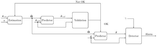
Figure 3.
Diagram of the modeling and detection method.
Given the model order n, the parameter vector is estimated from the signal . In the case of an ARFIMA model, the order is defined by . This will be further explained in Section 4.1.
Using a validation dataset , the model predictions are computed. Comparison between the real and the predicted signals, through the validation step, is necessary to evaluate the accuracy of the estimated model. If the validation step is successful, the model can be further used for prediction and detection or else the estimation step shall be repeated. A model issued after the validation step will be further used in a detection method. The detector generates an alarm depending on the result of the comparison between a well-defined statistical test and a threshold .
The choice of the threshold is decisive in the AD method. Generation of an alarm in case of an anomaly depends on the detector and the selected threshold. For the evaluation of the two variants of the new AD method, a complete spectrum of different threshold values is used as explained in Section 6.3.
The ARFIMA model was described in Section 4.1. According to Haslett and Raftery [41] an approximate one-step ARFIMA predictor of is given by
with
where represents the gamma (generalized factorial) function that is defined in Equation (11).
The prediction errors can be derived by replacing Equation (21) in Equation (13). Then, by maximizing Equation (14), an estimation of the parameter vector is obtained.
The MLE of an ARFIMA model can be estimated numerically. For the computations of the ARFIMA MLE, approximations have been developed such as [41,42]. An overview of different likelihood-based methods for estimation of long-memory time series models was presented in [43]. Since the statistical hypothesis testing considered in this work depends on the MLE of the ARFIMA model, a numerical approximation will be used.
5. Statistical Hypothesis Testing for the AD Method
The network traffic in electrical substations based on IEC 61850 can be described using an ARFIMA model as introduced in Section 4.
In order to detect DoS attacks in the communication network of electrical substations, we seek a relevant approach to formulate this scenario as a detection problem. The main idea is to distinguish between presence or absence of anomaly using two competing hypotheses. The hypothesis , referred to as the null hypothesis, indicates absence of anomaly, whereas indicates presence of an anomaly. Since the noise parameters are assumed to be unknown, the detection problem is thus referred to as the composite hypothesis testing [39].
For the statistical AD method, we use two well-known detectors namely Generalized Likelihood Ratio Test (GLRT) and Cumulative sum (CUSUM).
The GLRT decides for if
with a threshold which shall be chosen as a compromise between the Detection Rate (DR) and FAs. The term contains the ARFIMA parameters as well as the noise variance.
The numerator and denominator in Equation (23) represent the PDF under the hypotheses and , respectively. Since the occurrence time of an anomaly is unknown, the GOOSE traffic measurements should be analyzed sequentially for computation of Equation (23). In this work, two approaches of Equation (23) are proposed for the AD. In both approaches, the hypothesis is evaluated sequentially in two subsets as the change time is unknown.
In the first approach, referred to as the GLRT detector (D_G), the hypotheses in Equation (23) are defined as follows:
where is the MLE of under each hypothesis. The parameter vector is . The change time denoted by is unknown and should be investigated using Equation (23) whose hypotheses are evaluated with Equation (24).
As shown in Equation (24), in the time series is assumed not to have any change since the parameter vector is assumed to be the same among the entire dataset. In contrast, a change in is assumed to occur in which represents a possible anomaly in the process. The MLE under each hypothesis can be numerically computed for the ARFIMA model. Several algorithms for computation of the MLEs can be found in e.g., [39,40].
The AD algorithm is described in Figure 4 and explained in the following steps:
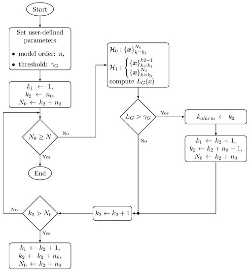
Figure 4.
Flow diagram of the statistical AD method based on the GLRT test.
- The algorithm starts by setting the user-defined parameters which are the order of the ARFIMA model i.e., n and a threshold which is defined empirically based on test results for FAs and DR.
- The null-hypothesis is computed with data contained between and . is computed using two data subsets: the bounds of the first one are represented by and and the second one is evaluated between and . Models for and are computed according to Equation (24) whilst .
- is computed as the ration between the pdf of each hypothesis as described in Equation (23). If holds, a change time is assigned to and an alarm is generated. The bounds of the dataset for and are also updated for further computations.
- If does not hold, is incremented and is computed in a new iteration. This procedure is repeated until and the bounds of the datasets for the computation of the PDFs in each hypothesis are updated.
The CUSUM algorithm, first presented in [44], is used as a detector (D_C) in the second variant of the AD approach. The CUSUM decides for if
with a user-defined threshold and the decision function defined by:
The decision function is initialized by and reset each time the condition Equation (25) holds.
The log-likelihood ratio increment is expressed in Equation (27) according to [45]:
and are the residuals and sample variance at time k for the i-th hypothesis. The model output is computed using Equation (21). In our case and most of the practical cases, the model parameters are unknown prior to the experiment, MLE estimates are used instead.
The AD algorithm based on the CUSUM detector is shown in Figure 5 and described as follows:
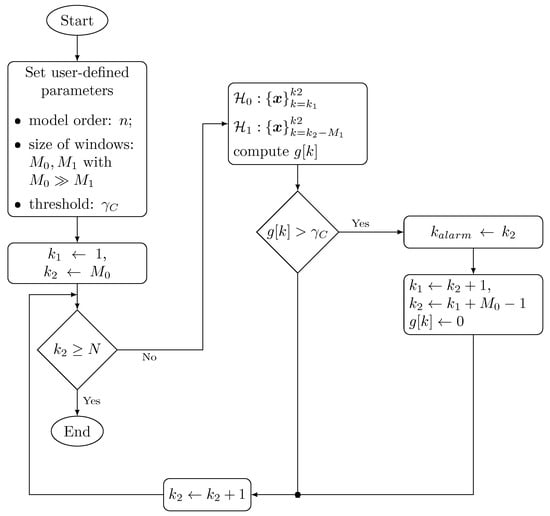
Figure 5.
Flow diagram of the statistical AD method based on the CUSUM test.
- The algorithm starts by setting the user-defined parameters which are the order of the ARFIMA model i.e., and the size of the time windows, and used for data scanning. The threshold is defined empirically based on test results for FAs and DR.
- As reported in [45], the model for is computed using a dataset defined by a growing time window whereas the model for is computed with data contained in a sliding fixed-size time window . Bounds of the datasets used for the computation of models for both hypothesis are represented by and . Models for and are computed while holds.
- The decision function is computed iteratively according to Equation (26). If holds, an alarm is generated indicating that anomaly is detected.
- Once an anomaly is detected, the detection time is set, the bounds and are updated and the detection function is reset.
This algorithm is able to detect multiple anomalies at unknown change times and assuming unknown noise parameters.
6. Results and Discussion
In this section, the proposed use case is first described including the generation of the network traffic in IEC 61850 substations as well as the perpetrated DoS attack. Then, performance evaluation of the AD method with both variants GLRT and CUSUM, is presented.
6.1. Description of the Use Case and the Threat Model
We use in the present work a synthesized dataset generated by the Advanced Digital Sciences Center (ADSC) [46]. The testbed describes the operation of a 66/11 kV electrical substation model including circuit breakers and IEDs. A typical network architecture was adopted using the recommended protocols in IEC 61850 standard i.e., GOOSE and SV communication between CTs, VTs and IEDs via Ethernet VLAN and MMS protocol at the station level for the connection between Human–Machine Interfaces (HMIs) and IEDs. All 18 simulated IEDs are within the same multicast group.
The GOOSE data traffic shown in black in Figure 6 describes an attack-free scenario. The normal operation in an electrical substation might also include disturbances such as a breaker failure or a busbar protection where specific GOOSE messages are sent to address such event changes.
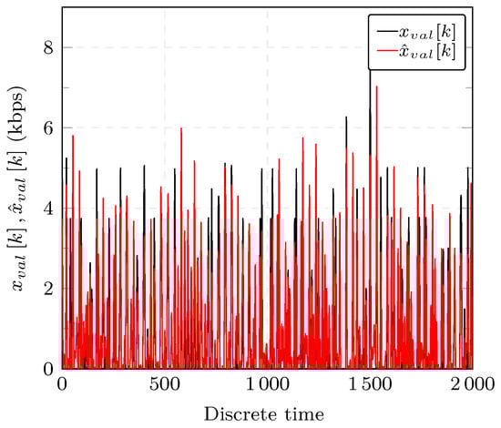
Figure 6.
GOOSE network traffic used for estimation (depicted in black) and arfima model prediction (depicted in red).
Normal operation in the electrical substation might be hindered by disturbances or malicious actions. In the following, a description of the considered threat model is introduced. In modern electrical substations, HMIs are equipped with monitoring and control interfaces that are remotely accessible. Attackers are assumed to be able to compromise this entry point through, for instance, social engineering in order to connect to IEDs. Among others, a DoS attack on the GOOSE communication was simulated and resulting network data was recorded. For our adversary model, a DoS attack on the the GOOSE communication is simulated.
Different variants of this attack are reported in the literature. Poisoning attack reported in [1] can result in a DoS when an attacker injects a spoofed GOOSE packet with a very high status number (StNum). Another variant is the high rate flooding attack that injects multiple GOOSE packets with incremental StNum that exceed the StNum of a legitimate packet. The last situation, called semantic attack, is based on monitoring the network traffic and spoofing the GOOSE packets with a higher rate of changing StNum than the normal. This would result in preventing subscribers from processing legitimate packets. Another variant of GOOSE DoS attack is demonstrated in [47] by causing an IED to lose availability due to the injection of a consequent number of GOOSE packets that is greater that the limit allowed for the packet transmission time.
The simulated attack was generated synthetically using an attack-free network scenario, an attack script and a traffic attack replay tool such as tcp replay. An automatic trace generator program is used to get an attack-induced trace by injecting malicious GOOSE packets. The attack model is based on compromising the GOOSE communication. By spoofing the transmitted messages, the attacker can masquerade a legitimate IED to inject maliciously crafted GOOSE messages. There are several ways to perpetrate a DOS attack. In the considered case, the simulated DoS results from flooding the network with bogus frames. More details about the generation framework of the different attack and attack-free scenarios can be found in [46]. Impact of losing availability in critical infrastructures’ networks can be much more severe than, for instance, in commercial systems.
6.2. Evaluation of the Modeling of GOOSE IEC 61850 Traffic
We evaluate the model using the data presented in Section 6.1. The dataset used for validation is denoted by in Figure 3 which represents GOOSE network traffic in SCN. Figure 6 shows the output of the ARFIMA model for the validation GOOSE traffic, , in red, and the dataset used for comparison in black.
To further assess the goodness-of-fit of the model, the following criterion is used:
where a perfect fit is 100%. Thereby the Normalized Root Mean Square Error (NRMSE) is defined by:
with being the sample mean of the validation dataset, the measured GOOSE network traffic at time k and the model prediction. The fit of the data to the ARFIMA model as expressed in Equation (28) yields 73.65% which indicates that the chosen model can describe well the time series.
In addition to the model fit, an analysis of the residuals confirms the adequacy of the chosen ARFIMA model. The residuals obtained in the validation step are computed using the predictor of the model with the parameters and a validation dataset .
The Auto-Correlation Function (ACF) of the residuals are computed and shown in Figure 7. The ACF of (see Equation (13)) falls into the confidence level which indicates that the residuals can be considered as WGN and confirms that the model describes the GOOSE traffic data satisfactorily.
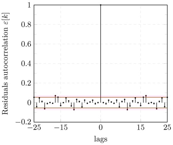
Figure 7.
Auto-correlation of ARFIMA model residuals.
6.3. Performance of the Anomaly Detection (AD) Method
We evaluate the performance of the proposed statistical AD methods, GLRT and CUSUM, using several criteria that are further discussed.
A FA indicates that is chosen when is true. FAs are also referred to as false positives (FPs). True positives (TPs) (i.e., a hit) refer to the fact that the detector decides correctly for . A true negative (TN) (i.e., correct rejection) indicates that is correctly rejected. A false negative (FN) (i.e., miss) occurs when is chosen when is true. Those concepts will be further used to define some assessment criteria.
Accuracy, one of the performance metrics considered, refers to the frequency with which the detector identifies properly the anomaly. However, accuracy might be misleading for the assessment of the AD method in case of a high imbalance between FP and FN.
When the cost of FNs is high, the True Positive Rate (TPR) also called DR or recall might help give additional information about the model. The True Negative Rate (TNR), also called specificity, indicates the proportion of correctly classified nonanomalous samples w.r.t. the total number of samples of the dataset. The False Positive Rate (FPR) represents the rate of FAs which is referred to as type I errors in statistics. False Negative Rate (FNR) or miss rate represents the proportion of type II error, i.e., is chosen when is true.
The computation of the different performance metrics are presented in the following:
The detection time is another performance indicator used to assess AD algorithms and describes the instant when an anomaly is detected.
Several experiments including a DoS attack at time are generated using the ARFIMA model previously described. WGN with sample variance derived from the estimated model is used for simulation. The performance of the GLRT and CUSUM detectors defined in Equations (24) and (26), is evaluated for several thresholds s.
The experiments are performed using the R programming language version 3.6.2 on an Intel i7-2.00 GHz with 32 GB RAM. A total number of 25 Monte-Carlo simulations are performed for each threshold and under different realizations of WGN for each experiment. A realization of one of the experiments is shown in Figure 8. The result of the two proposed detectors for one of the experiments is shown in Figure 9 and Figure 10.
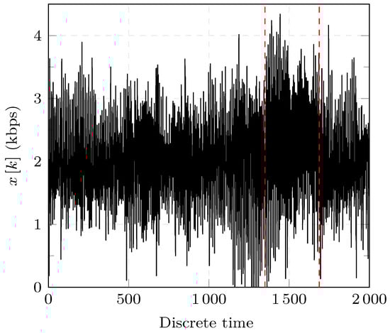
Figure 8.
Simulated GOOSE network traffic with a DOS attack.
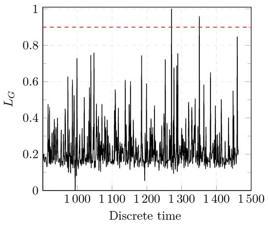
Figure 9.
Results of the GLRT detection test.
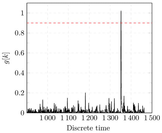
Figure 10.
Results of the CUSUM detection test.
Before a change occurs, the values of and oscillate within a certain range. When a change occurs, the values of both detectors change abruptly which indicates that an anomaly was successfully detected as shown in Figure 9 and Figure 10. In case of the CUSUM detector as shown in Figure 10, no FAs were present. In Figure 9, the first peak represents a FA as the value of exceeds the threshold (dashed red line). The test statistic is reset in the CUSUM detection approach after a change is detected. Further changes can be, thus, detected.
It is worth noting that both approaches are able to detect several changes. However, in the specific case of a DoS attack, we are interested in detecting the first change as shown in Figure 4 and Figure 5.
To evaluate the performance of our AD method, three scenarios with different signal-to-noise ratios (SNRs) are considered.
The SNR is defined by:
where and are the variances of the signal x and noise e, respectively.
The performance of the CUSUM and GLRT detectors under different SNRs can be observed using the Receiver Operating Characteristic (ROC) plot. ROC plots help describe the tradeoff between FPR and FNR over a complete spectrum of operating conditions including the settings of the decision threshold. The ROC curve represents the relation between the probability of detection i.e., TPR and the probability of false alarm i.e., FPR to help assess the performance of the detectors depending on the requirements of the application. An algorithm is considered to be good if the ROC curve reaches rapidly the upper left-hand corner i.e., if the area under the curve is large. Under simple assumptions such as the analysis of a signal embedded in Gaussian noise, the ROC curve can be typically derived analytically. This is not the case in our work as we are using a more complex model that requires experimental computation of the ROC curve. The performance of both detectors degrades, overall, for lower SNR values, i.e., a high noise content is shown in Figure 11 and Figure 12. This can be explained by high deviations of the estimates with respect to the true values when the noise variance increases.
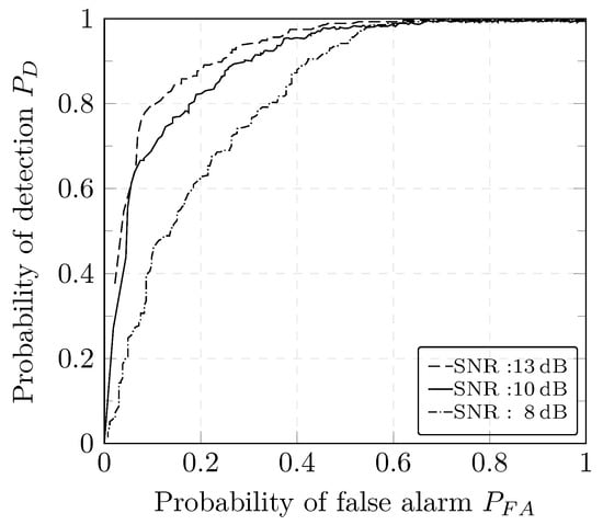
Figure 11.
ROC curve of the GLRT detector.
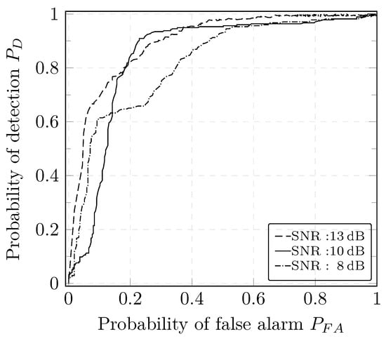
Figure 12.
ROC curve of the CUSUM detector.
For different case studies, authors in [16] report a detection rate of 100%; however, a hybrid approach using whitelisting and deep packet inspection (DPI) is adopted. Similar detection results are reported in [48] with the use of critical state analysis that are based on a comprehensive description of the physical models of the considered power system. Our technique proposed in the present work has a comparable detection rate as other approaches for detection of DoS attacks. However, a major advantage of our method is that we do not require to include DPI or to build a set of rules that need to be constantly maintained.
To achieve a good performance, IDSs based on ML approaches generally use supervised algorithms which require two different datasets for the training of the detection algorithm. This is a considerable limitation as they increase the deployment and operational costs.
Our AD statistical method is compared with the most relevant approaches available in the literature ([21,29]) and the results are listed in Table 1.

Table 1.
Comparison of detection results with available methods.
In [21,29], statistical AD methods for the detection of attacks in 61,850 substations, are proposed. In [21], the authors present a statistical detection based on a comparison of the residuals with a variance-based threshold while assuming a model to describe a signal embedded in WGN for the network traffic. In contrast to [21], where the residuals are obtained from a signal embedded in WGN, we consider a modified version with the residuals computed from our ARFIMA model.
The approach presented in [29] is based on an anomaly score resulting from the comparison of the network traffic with a minimum and a maximum value extracted from real measurements. No details were provided in [29] for the choice of the user-defined parameters necessary for the anomaly detection score. Thus, we choose empirically adapted values that would allow a high probability of anomaly detection for the considered case study. We implemented both approaches for comparison with our method which has two different variants as defined in Section 5. Under similar operating conditions and using the same scenario, the results of 25 Monte-Carlo simulations are presented in Table 1.
Table 1 shows the performance of the detectors for SNR = 10 dB. The first column in Table 1 represents normalized values of the thresholds for the AD methods.
The detection time for the CUSUM and GLRT is defined when the conditions in Equations (23) and (25) hold. The delay time is expressed in samples and it represents the number of discrete time samples after which the anomaly is detected. The wider the window size for data scanning is, the larger the detection delay is. However, the detection statistics such as the accuracy improve with larger window size. Thus, there should be a compromise between the detection delay and the detection statistics. The average delay in the detection time of the CUSUM is around 1.6% smaller than in the GLRT test.
For a better readability of the different results, we only include in Table 1 the FPR and the FNR as the other basic detection criteria can be directly concluded from Equation (30d). On average, the detection delay obtained from the modified approach introduced in [21] is the smallest. It is around 5.8% faster than our approach with the CUSUM variant. The largest detection delay is obtained for the approach developed in [29] which is, on average, 30% slower than our modified version of [21]. The quick detection delay in the modified [21] can be explained by the direct comparison of the residuals with a threshold. In contrast, detection tests in other approaches are computed using the residuals processed in data windows. Our approach based on CUSUM test (D_C) performs better than the D_G approach w.r.t. the detection delay.
Our D_G approach has, on average, the lowest FPR with a value of 6.66%. The FPR of the detection algorithm presented in [29] is the highest with a value of 14.92% whereas for our AD approach based on the GLRT detector, it is around 7.72%.
The AD based on the CUSUM detector exhibits the lowest average FNR with a value of 7.4% thus the highest DR with a value of 92.6%. The modified approach from [21] has a slightly higher FNR than our AD with a value of around 7.56%. The FNR of the GLRT detector is 0.72% higher than the CUSUM detector. This can be explained by the fact that the CUSUM test uses values of previous computation of the test statistics as expressed in Equation (26).
In summary, our approach based on the GLRT detector has the the lowest FPR whereas the one based on the CUSUM test has the lowest FNR when compared with [21,29]. Thus, to better compare the performance of the IDSs, we use the two composite detection metrics presented in [49]. The composite metrics give an overall overview of the detection performance and are computed using the basic performance criteria. Those additional metrics do not, however, replace the basics ones [50]. The expected cost metric, , required a user-defined parameter C which is the ratio of the cost of an IDS failing to detect an intrusion and the the cost when an IDS generates an alert when an intrusion has not occurred. The expected cost metric is computed as follows:
where is the base rate, i.e., the probability that there is an intrusion in the observed dataset. For our experiments, we consider that the cost of a FNR is much higher than the cost of FPR, i.e., the value of C is chosen to be equal to 10 following [49]. To compare the performance of the different IDSs, the approach with the lowest is considered to be the best [49]. The minimal value of for each approach is shown in bold in the Table 1. Our AD based on the GLRT detector has the lowest expected cost compared with the other AD methods. Although the cost-based metric gives a practical way to relate the different basic metrics to compare the performance of IDSs, it is however dependent on the subjective measure C. The ratio of the cost of an IDS failing to detect an intrusion and the the cost of generating a FA can be difficult to define as it depends on several factors such as the number of working hours, man-power cost, etc.
A second composite metric , first introduced in [50], provides a more objective evaluation of the performance of the considered IDSs. The intrusion detection capability presents the ratio of the mutual information between the IDS input and output to the entropy of the input. For derivation details of this metric, the reader can refer to [50]. To compare IDSs, the maximum value of obtained for each approach shall be compared between them. The maximum value of for each approach is depicted in bold in Table 1. The value of of our AD approach based on the GLRT detector is around which is the highest value among all the considered approaches. This observation supports the results concluded from the first composite metric . Under similar operating conditions, our novel AD approach based on the GLRT test is experimentally proved to perform better than [21,29] for the detection of DoS attacks.
7. Conclusions & Outlook
Increased use of ICT in ICS in general and in SCADA critical infrastructures in particular have considerably improved the interconnection between the different components. Power systems are highly dependent on digital control, supervision and monitoring for a safe and optimal operation. Some of the networking protocols used in this sector were not primarily designed with security in mind which exposed the whole power grid domain as an attractive target for attackers. In order to help improve the Cyber-Physical Security (CPS) of the Smart Grid (SG), the present work tackles the challenge to enhance the availability of the data in communication networks in electrical substations based on IEC61850.
We introduce a structured analysis of the Substation Communication Network (SCN) traffic in order to gather necessary knowledge about the description of the GOOSE network traffic. Based on the studied characteristics, we discuss the Auto-Regressive Fractionally Integrated Moving Average (ARFIMA) model to mathematically describe the GOOSE network traffic in IEC 61850 electric substations. Our modeling of the communication network supports the research in forecasting the traffic with a high accuracy and in designing the GOOSE network architecture of electrical substations. The estimated ARFIMA model is evaluated on a simulation case study representing a substation testbed.
The obtained model is used for developing an Anomaly Detection (AD) based on statistical hypothesis testing. We apply two different approaches for the AD namely, the Generalized Likelihood Ratio Test (GLRT) and the CUSUM test. The statistical AD method with both detectors is able to successfully locate Denial of Service (DoS) and other flooding attacks on a simulation use case that includes a Denial of Service (DoS) attack. Based on the implemented simulations, both detectors were shown to have better performance in terms of basic and composite detection metrics as well as detection delay, when compared with available approaches.
Author Contributions
Conceptualization, G.E. and H.B.K.; methodology, validation and writing G.E.; review and editing, G.E., H.B.K., A.B., K.N. and V.H.; supervision H.B.K., K.N. and V.H.; funding acquisition, H.B.K., K.N. and V.H. All authors have read and agreed to the published version of the manuscript.
Funding
This research was partially funded by Helmholtz Programm Energieeffizienz, Materialien und Ressourcen EMR (34.15.01), Kastel BMBF Projekt Sicherheit kritischer Infrastrukturen SKI, BMBF Energiesystem 2050 and the Karlsruhe House of Young Scientists (KHYS). This material is based upon work partially supported by the Department of Energy’s Office of Cybersecurity, Energy Security, and Emergency Response and the Department of Homeland Security’s Security Science & Technology Directorate under Award Number DE-OE0000780. The views and opinions of authors expressed herein do not necessarily state or reflect those of the United States Government or any agency thereof. We also acknowledge support by the KIT-Publication Fund of the Karlsruhe Institute of Technology.
Acknowledgments
The authors would like to thank the anonymous reviewers who kindly reviewed the earlier version of this manuscript and provided valuable suggestions and comments. We would also like to thank Alfonso Valdes for his constructive feedback and his insightful comments.
Conflicts of Interest
The authors declare no conflict of interest.
Abbreviations
| ACF | Auto-Correlation Function |
| AD | Anomaly Detection |
| CPS | Cyber-Physical Security |
| CUSUM | Cumulative sum |
| DoS | Denial of Service |
| DPI | Deep Packet Inspection |
| GLRT | Generalized Likelihood Ratio Test |
| GOOSE | Generic Object Oriented Substation Event |
| HMI | Human-Machine Interface |
| ICS | Industrial Control System |
| ICT | Information and Communication Technology |
| IEC | International Electrotechnical Commission |
| IED | Intelligent Electronic Device |
| LRD | Long-Range Dependency |
| ML | Machine-Learning |
| MLE | Maximum Likelihood Estimator |
| MMS | Manufacturing Message Specification |
| MU | Merging Unit |
| NRMSE | Normalized Root Mean Square Error |
| Probability Density Function | |
| ROC | Receiver Operating Characteristic |
| RT | Real-Time |
| SCADA | Supervisory Control And Data Acquisition |
| SCN | Substation Communication Network |
| SG | Smart Grid |
| SRD | Short-Range Dependency |
| SV | Sampled Values |
| TNR | True Negative Rate |
| TPR | True Positive Rate |
| WGN | White Gaussian Noise |
| Glossary | |
| B | Backshift operator. |
| The intrusion detection capability metric. | |
| The expected cost metric. | |
| H | Hurst parameter. |
| L | Length of non-overlaping intervals composing a time-series. |
| Initial size of the dataset for the calculation of the CUSUM detector. | |
| Length of fixed-sized sliding window for the calculation of the CUSUM detector. | |
| N | Size of a time-series. |
| The standard deviation of a subset x calculated over the interval . | |
| The partial sum of a subset x calculated over the interval . | |
| The gamma (generalized factorial) function. | |
| The covariance matrix of the measurement noise. | |
| Moving average (MA) polynomial operator of an ARFIMA model. | |
| The parameter vector. | |
| Model residuals. | |
| x | Time-series. |
| The aggregated sequence by m of x. | |
| B | The base rate. |
| The threshold for the CUSUM statistical detection. | |
| The threshold for the GLRT statistical detection. | |
| Sample mean. | |
| Sample variance. | |
| Autoregressive (AR) polynomial operator of an ARFIMA model. | |
| Variance of a white Gaussian noise process. | |
| d | The difference coefficient. |
| Value of e at k. | |
| g | The CUSUM decision function. |
| k | Discrete time index. |
| Time at which an attack occurs. | |
| l | Delay order of the back-shift operator. |
| m | The level of aggregation. |
| n | ARFIMA model order defined by . |
| p | The order of the autoregressive process. |
| q | The order of moving the average. |
| Log-likelihood ratio increment. |
References
- Hoyos, J.; Dehus, M.; Brown, T.X. Exploiting the GOOSE protocol: A practical attack on cyber-infrastructure. In Proceedings of the Globecom Workshops (GC Wkshps), Anaheim, CA, USA, 3–7 December 2012; IEEE: New York, NY, USA, 2012; pp. 1508–1513. [Google Scholar]
- Elbez, G.; Keller, H.B.; Hagenmeyer, V. A New Classification of Attacks against the Cyber-Physical Security of Smart Grids. In Proceedings of the ARES 2018: International Conference on Availability, Reliability and Security, Hamburg, Germany, 27–30 August 2018. [Google Scholar]
- Yoo, H.; Shon, T. Challenges and research directions for heterogeneous cyber–physical system based on IEC 61850: Vulnerabilities, security requirements, and security architecture. Future Gener. Comput. Syst. 2016, 61, 128–136. [Google Scholar] [CrossRef]
- Keller, H.B.; Schneider, O.; Matthes, J.; Hagenmeyer, V. Reliable, safe and secure software of connected future control systems-challenges and solutions. at-Automatisierungstechnik 2016, 64, 930–947. [Google Scholar] [CrossRef]
- Cherepanov, A.; Lipovsky, R. Industroyer: Biggest Threat to Industrial Control Systems Since Stuxnet. WeLiveSecurity by ESET. 2017. Available online: https://www.welivesecurity.com/2017/06/12/industroyer-biggest-threatindustrial-control-systems-since-stuxnet/ (accessed on 24 October 2018).
- Elbez, G.; Keller, H.B.; Hagenmeyer, V. Authentication of GOOSE Messages under Timing Constraints in IEC 61850 Substations. In Proceedings of the 6th International Symposium for ICS & SCADA Cyber Security Research, Athens, Greece, 10–12 September 2019; pp. 137–143. [Google Scholar]
- Ustun, T.S.; Aftab, M.A.; Ali, I.; Hussain, S.S. A Novel Scheme for Performance Evaluation of an IEC 61850-Based Active Distribution System Substation. IEEE Access 2019, 7, 123893–123902. [Google Scholar] [CrossRef]
- Pal, A.; Jolfaei, A.; Kant, K.; Chi, H. A Fast Prekeying Based Integrity Protection for Smart Grid Communications. Available online: https://cis.temple.edu/~apal/SmartGrid_security.pdf (accessed on 29 June 2020).
- Nguyen, H.; Pongthawornkamol, T.; Nahrstedt, K. Alibi framework for identifying reactive jamming nodes in wireless LAN. In Proceedings of the 2011 IEEE Global Telecommunications Conference-GLOBECOM, Houston, TX, USA, 5–9 December 2011; IEEE: Houston, TX, USA, 2011; pp. 1–6. [Google Scholar]
- Castaño, F.; Strzelczak, S.; Villalonga, A.; Haber, R.E.; Kossakowska, J. Sensor reliability in cyber-physical systems using internet-of-things data: A review and case study. Remote Sens. 2019, 11, 2252. [Google Scholar] [CrossRef]
- Basseville, M. Detecting changes in signals and systems—A survey. Automatica 1988, 24, 309–326. [Google Scholar] [CrossRef]
- Cheung, S.; Dutertre, B.; Fong, M.; Lindqvist, U.; Skinner, K.; Valdes, A. Using Model-Based Intrusion Detection for SCADA Networks. Available online: http://citeseerx.ist.psu.edu/viewdoc/download?doi=10.1.1.141.2076&rep=rep1&type=pdf (accessed on 24 September 2020).
- Premaratne, U.K.; Samarabandu, J.; Sidhu, T.S.; Beresh, R.; Tan, J.C. An intrusion detection system for IEC61850 automated substations. IEEE Trans. Power Deliv. 2010, 25, 2376–2383. [Google Scholar] [CrossRef]
- Morris, T.; Vaughn, R.; Dandass, Y. A retrofit network intrusion detection system for MODBUS RTU and ASCII industrial control systems. In Proceedings of the 2012 45th Hawaii International Conference on System Sciences, Maui, HI, USA, 4–7 January 2012; IEEE: Maui, HI, USA, 2012; pp. 2338–2345. [Google Scholar]
- Lin, H.; Slagell, A.; Di Martino, C.; Kalbarczyk, Z.; Iyer, R.K. Adapting bro into scada: Building a specification-based intrusion detection system for the dnp3 protocol. In Proceedings of the Eighth Annual Cyber Security and Information Intelligence Research Workshop, Oak Ridge, TN, USA, 8–10 January 2013; pp. 1–4. [Google Scholar]
- Yang, Y.; Xu, H.Q.; Gao, L.; Yuan, Y.B.; McLaughlin, K.; Sezer, S. Multidimensional intrusion detection system for IEC 61850-based SCADA networks. IEEE Trans. Power Deliv. 2016, 32, 1068–1078. [Google Scholar] [CrossRef]
- Nivethan, J.; Papa, M. Dynamic rule generation for SCADA intrusion detection. In Proceedings of the 2016 IEEE Symposium on Technologies for Homeland Security (HST), Waltham, MA, USA, 10–11 May 2016; IEEE: Waltham, MA, USA, 2016; pp. 1–5. [Google Scholar]
- Barbosa, R.R.R. Anomaly Detection in SCADA Systems: A Network Based Approach. 2014. Available online: https://research.utwente.nl/en/publications/anomaly-detection-in-scada-systems-a-network-based-approach-2 (accessed on 29 June 2020).
- Shang, W.; Zeng, P.; Wan, M.; Li, L.; An, P. Intrusion detection algorithm based on OCSVM in industrial control system. Secur. Commun. Netw. 2016, 9, 1040–1049. [Google Scholar] [CrossRef]
- Shang, W.; Li, L.; Wan, M.; Zeng, P. Industrial communication intrusion detection algorithm based on improved one-class SVM. In Proceedings of the 2015 World Congress on Industrial Control Systems Security (WCICSS), London, UK, 14–16 December 2015; IEEE: London, UK, 2015; pp. 21–25. [Google Scholar]
- Kwon, Y.; Kim, H.K.; Lim, Y.H.; Lim, J.I. A behavior-based intrusion detection technique for smart grid infrastructure. In Proceedings of the 2015 IEEE Eindhoven PowerTech, Eindhoven, The Netherlands, 29 June–2 July 2015; IEEE: Eindhoven, The Netherlands, 2015; pp. 1–6. [Google Scholar]
- Ren, W.; Yardley, T.; Nahrstedt, K. EDMAND: Edge-Based Multi-Level Anomaly Detection for SCADA Networks. In Proceedings of the 2018 IEEE International Conference on Communications, Control, and Computing Technologies for Smart Grids (SmartGridComm), Aalborg, Denmark, 29–31 October 2018; pp. 1–7. [Google Scholar]
- Coughlin, V.; Rubio-Medrano, C.; Zhao, Z.; Ahn, G.J. EDSGuard: Enforcing Network Security Requirements for Energy Delivery Systems. In Proceedings of the 2018 IEEE International Conference on Communications, Control, and Computing Technologies for Smart Grids (SmartGridComm), Aalborg, Denmark, 29–31 October 2018; IEEE: Aalborg, Denmark, 2018; pp. 1–6. [Google Scholar]
- Yang, Y.; McLaughlin, K.; Gao, L.; Sezer, S.; Yuan, Y.; Gong, Y. Intrusion detection system for IEC 61850 based smart substations. In Proceedings of the 2016 IEEE Power and Energy Society General Meeting (PESGM), Boston, MA, USA, 17–21 July 2016; IEEE: Boston, MA, USA, 2016; pp. 1–5. [Google Scholar]
- Zhang, Z.; Huang, X.; Keune, B.; Cao, Y.; Li, Y. Modeling and simulation of data flow for vlan-based communication in substations. IEEE Syst. J. 2015, 11, 2467–2478. [Google Scholar] [CrossRef]
- Floyd, S.; Paxson, V. Difficulties in simulating the Internet. IEEE/ACM Trans. Netw. 2001, 9, 392–403. [Google Scholar] [CrossRef]
- IEC61850. International Electrotechnical Commission (IEC) Technical Committee 57; Communication Networks and Systems in Substations—Part 5: Communication Requirements for Functions and Device Models. 2003. Available online: https://webstore.iec.ch/preview/info_iec61850-5%7Bed1.0%7Den.pdf (accessed on 29 June 2020).
- Willinger, W.; Taqqu, M.S.; Sherman, R.; Wilson, D.V. Self-similarity through high-variability: Statistical analysis of Ethernet LAN traffic at the source level. IEEE/ACM Trans. Netw. 1997, 5, 71–86. [Google Scholar] [CrossRef]
- Yang, Q.; Hao, W.; Ge, L.; Ruan, W.; Chi, F. FARIMA model-based communication traffic anomaly detection in intelligent electric power substations. IET Cyber-Phys. Syst. Theory Appl. 2019, 4, 22–29. [Google Scholar] [CrossRef]
- Hao, W.; Yang, Q. Data Traffic Characterization in Intelligent Electric Substations using FARIMA based Threshold Model. Energy Procedia 2018, 145, 413–420. [Google Scholar] [CrossRef]
- Feizimirkhani, R.; Bratcu, A.I.; Besanger, Y. Time-series Modelling of IEC 61850 GOOSE Communication Traffic between IEDs in smart grids—A parametric analysis. IFAC Pap. 2018, 51, 444–449. [Google Scholar] [CrossRef]
- Hurst, H.E. Long-term storage capacity of reservoirs. Trans. Am. Soc. Civ. Eng. 1951, 116, 770–799. [Google Scholar]
- Leland, W.E.; Taqqu, M.S.; Willinger, W.; Wilson, D.V. On the self-similar nature of Ethernet traffic (extended version). IEEE/ACM Trans. Netw. 1994, 2, 1–15. [Google Scholar] [CrossRef]
- Mandelbrot, B. Statistical methodology for nonperiodic cycles: From the covariance to R/S analysis. In Annals of Economic and Social Measurement, Volume 1, Number 3; NBER: Cambridge, MA, USA, 1972; pp. 259–290. [Google Scholar]
- Lloyd, E.; Warren, D. The historically adjusted range and the historically rescaled adjusted range. Stoch. Hydrol. Hydraul. 1988, 2, 175–188. [Google Scholar] [CrossRef]
- Boubaker, H. A generalized arfima model with smooth transition fractional integration parameter. J. Time Ser. Econom. 2017, 10. [Google Scholar] [CrossRef]
- Hosking, J. Fractional differencing modeling in hydrology 1. JAWRA J. Am. Water Resour. Assoc. 1985, 21, 677–682. [Google Scholar] [CrossRef]
- Goodwin, G.C.; Payne, R.L. Dynamic System Identification. Experiment Design And Data Analysis. 1977. Available online: https://pascal-francis.inist.fr/vibad/index.php?action=getRecordDetail&idt=PASCAL7830233130 (accessed on 29 June 2020).
- Kay, S.M. Fundamentals of Statistical Signal Processing; Prentice Hall PTR: Upper Saddle River, NJ, USA, 1993. [Google Scholar]
- Söderström, T.; Stoica, P. System Identification; Prentice-Hall Inc.: London, UK, 1988. [Google Scholar]
- Haslett, J.; Raftery, A.E. Space-time modelling with long-memory dependence: Assessing Ireland’s wind power resource. J. R. Stat. Soc. Ser. C Appl. Stat. 1989, 38, 1–21. [Google Scholar] [CrossRef]
- Fox, R.; Taqqu, M.S. Large-sample properties of parameter estimates for strongly dependent stationary Gaussian time series. Ann. Stat. 1986, 14, 517–532. [Google Scholar] [CrossRef]
- Chan, N.H.; Palma, W. Estimation of long-memory time series models: A survey of different likelihood-based methods. Adv. Econom. 2006, 20, 89–121. [Google Scholar]
- Page, E.S. Continuous inspection schemes. Biometrika 1954, 41, 100–115. [Google Scholar] [CrossRef]
- Basseville, M.; Nikiforov, I.V. Detection of Abrupt Changes: Theory and Application; Prentice Hall: Englewood Cliffs, NJ, USA, 1993; Volume 104. [Google Scholar]
- Biswas, P.P.; Tan, H.C.; Zhu, Q.; Li, Y.; Mashima, D.; Chen, B. A Synthesized Dataset for Cybersecurity Study of IEC 61850 based Substation. In Proceedings of the 2019 IEEE International Conference on Communications, Control, and Computing Technologies for Smart Grids (SmartGridComm), Beijing, China, 21–23 October 2019; IEEE: Beijing, China, 2019; pp. 1–7. [Google Scholar]
- Hong, J.; Liu, C.C.; Govindarasu, M. Integrated Anomaly Detection for Cyber Security of the Substations. IEEE Trans. Smart Grid 2014, 5, 1643–1653. [Google Scholar] [CrossRef]
- Carcano, A.; Coletta, A.; Guglielmi, M.; Masera, M.; Fovino, I.N.; Trombetta, A. A multidimensional critical state analysis for detecting intrusions in SCADA systems. IEEE Trans. Ind. Inform. 2011, 7, 179–186. [Google Scholar] [CrossRef]
- Milenkoski, A.; Vieira, M.; Kounev, S.; Avritzer, A.; Payne, B.D. Evaluating computer intrusion detection systems: A survey of common practices. ACM Comput. Surv. CSUR 2015, 48, 1–41. [Google Scholar] [CrossRef]
- Gu, G.; Fogla, P.; Dagon, D.; Lee, W.; Skorić, B. Measuring intrusion detection capability: An information-theoretic approach. In Proceedings of the 2006 ACM Symposium on Information, Computer and Communications Security, Taipei, Taiwan, 21–24 March 2006; pp. 90–101. [Google Scholar]


© 2020 by the authors. Licensee MDPI, Basel, Switzerland. This article is an open access article distributed under the terms and conditions of the Creative Commons Attribution (CC BY) license (http://creativecommons.org/licenses/by/4.0/).