Abstract
This paper deals with the problem of the leakage inductance calculations in power transformers. Commonly, the leakage flux in the air zone is represented by short-circuit inductance, which determines the short-circuit voltage, which is a very important factor for power transformers. That inductance is a good representation of the typical power transformer windings, but it is insufficient for multi-winding ones. This paper presents simple formulae for self- and mutual leakage inductance calculations for an arbitrary pair of windings. It follows from a simple 1D approach to analyzing the stray field using a discrete differential operator, and it was verified by the finite element method (FEM) calculation results.
1. Introduction
Power transformers are rather well-recognized electromagnetic devices. During the almost 150 year history of their development, countless books and papers have been devoted to power transformers, examples of which are [1,2,3,4]. Theoretical, design and operation problems have been solved. Besides the classical single-phase and three-phase, new types of power transformers have been designed for special applications: power system control, power electronics units, or electrical traction. Many of them have a lot of windings located in a common magnetic circuit. Three examples of transformers for power system control are shown in Figure 1a–c. The connection scheme of phase-shifting transformers to control the level and the phase of voltages is presented in Figure 1a. Figure 1b presents the connection scheme of multilevel autotransformers, and Figure 1c presents the connection of transformer windings for the HVDC transmission lines.
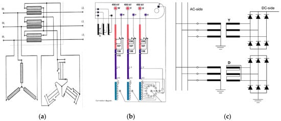
Figure 1.
Transformers for power system control (a) phase-shifting transformers (b) multilevel autotransformer (c) HVDC transformer.
Rectifier transformers generating multi-phase voltages or currents can also have many windings. Figure 2a,b show the provisional location of windings in the air window for Yyd 3/6-phase transformers and Figure 2b for Yzyd 3/12-phase transformers [5]. The location of the windings loses symmetry that is characteristic for classical three-phase power transformers. Single-phase traction transformers, to ensure various voltage levels on a traction vehicle at different traction supply systems, consist of many (up to 25) separate windings [6,7].
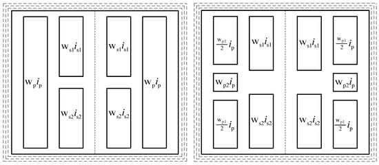
Figure 2.
Winding’s location in rectifier transformers (a) 3/6 phase transformers (b) 3/12 phase transformers.
Two approaches are used to recognize the properties of transformers. The first is based on the Maxwell equations for the magnetic vector potential. The second is based on the Kirchhoff equations for magnetically coupled coils. The first one is applied mainly for design problems of transformers, whereas the second is used for operation problems, when the transformer is a part of a multi-object system. These two approaches are combined by the set of the transformer’s parameters, which are lumped values combining the linked fluxes of the transformer’s windings with the winding currents. Due to the magnetic nonlinearity of the transformer’s ferromagnetic core, those relations are nonlinear and, in fact, can be determined by solving the Maxwell equations only. Nowadays, software packages for solving electromagnetic fields allow us to effectively find the magnetic field distribution in 2D or 3D space, also combining the Maxwell and the Kirchhoff equations [8,9,10,11,12,13,14]. However, it is rather cost- and time-consuming and seems to be unsuitable for solving operating problems in systems with power transformers. This is why the simplified approaches for calculations of the transformer’s parameters are often applied [15,16,17,18,19,20].
The most spectacular of these is the calculation of the short-circuit impedance of a typical power transformer. It is defined by two windings located on the same limb, assuming that ampere-turns of windings compensate at a sufficiently high magnetic permeability of the ferromagnetic transformer’s core. For such cases, the 1D field analysis in the air zone provides rather simple formulae for short-circuit reactances, which can be found in many books and textbooks on transformers, and are still recommended to designers. That approach has been successively applied to calculations of short-circuit impedances of multi-winding traction transformers [6,7]. Unfortunately, it is not valid at asymmetrical locations of windings in the air window. At least a 2D approach is necessary for that, which is presented in [21]. In this paper, an analytical solution of magnetic vector potential has been formulated for the transformer’s air window with arbitrarily located windings at zero Newmann boundary conditions on the ferromagnetic borders. To fulfil such boundary conditions, the ampere-turns of windings in the air window have to be balanced, i.e., their sum must equal zero. This allows us to calculate the short-circuit inductances for an arbitrary pair of windings. However, the leakage inductances of individual windings and the mutual inductances due to the stray field cannot be determined. To find those inductances, 2D or 3D field calculations across the entire magnetic circuit, including both the ferromagnetic core and the air zone, were applied [22].
To overcome the difficulties of 2D or 3D magnetic field computation, the relations between winding linked fluxes and currents , necessary for the Kirchhoff’s equations of transformers, can be presented in the form:
The first matrix represents inductances due to fluxes in the ferromagnetic core, and the second follows from the stray field in the air windows. The inductances are nonlinear when considering ferromagnetic core saturation and can depend on the currents of all the windings, whereas the inductances take constant values because the air zone is magnetically linear. Those two matrices can be calculated separately by a simplified approach. The first matrix only considers the nonlinear ferromagnetic core and omits the field in the air. The second matrix can be determined by considering the field in the air zone only, assuming that the permeability of the ferromagnetic core is sufficiently high, i.e., . This form of relations between linked fluxes and currents allows us to create the multi-port equivalent schemes of a multi-winding transformer with an arbitrary number of windings [23,24].
This paper presents an approach for determining inductances for symmetrically-located windings, when the Rogowski factor can be applied to correct the length of the magnetic path of stray flux in the air window. This is a modification of 1D analysis, which uses the discrete differential operator developed in [25,26]. Difficulties in formulating the boundary conditions for the case in which a magnetic field is generated by only one winding has been omitted. This is based on the result of test calculations using the finite element method (FEM) model that included the ferromagnetic plates around the air window. This method allows us to find simple formulae for self- and mutual leakage inductances for an arbitrary pair of windings and leads to the well-known form that many books formulate for the short-circuit inductance. This time though, each winding pair is represented by three values: two self-inductances and one mutual inductance instead of one short-circuit inductance. This way, all the elements of the leakage induction matrix in the relations (1) can be determined. It essentially improves the modeling of multi-winding transformers.
The paper is organized as follows: in the Section 2, the algebraic equations including leakage inductance for a pair of coupled windings are presented. In Section 3, the finite-difference equations are formulated which, with the help of method of images, ae used to find the magnetic potential in the case in which only one winding was excited in the air zone. Section 4 presents calculations of self- and mutual inductances due to fluxes in the air window based on energy stored in the air. Finally, conclusions are given in Section 5.
2. Description of Two Transformer Windings Accounting for Magnetic Coupling in the Air Zone
The phenomenon of magnetic coupling of transformer windings can be reduced to the case of two windings. A general equation of such a case is
To consider the coupling of these two windings by the fluxes in the air zone, the inductance matrix, using the relation (1), can be written in the form
assuming that . The inductances with subscript ‘μ’ follow from the flux in the magnetic core, whereas those with subscript ‘σ’, result from the flux in the air. By recalculating the parameters of the winding ‘2’ to the winding ‘1’ by the factor , the simplest relation can be obtained
Power transformers, beside the nominal voltages and currents, are characterized by a factor known as the short-circuit voltage, which is determined by so-called short-circuit impedance, mainly the short-circuit reactance . The short-circuit reactance is calculated for symmetrically designed power transformers commonly in the 1D approach, assuming that the currents of the two windings are balanced, i.e., omitting the magnetizing current. Such representation is valid for two windings located in the air window zone, for which the Rogowski factor can be satisfactory applied. The inductances , , and cannot be determined in that way. Usually, these inductances are approximated as and , based on the short-circuit inductance . However, it is insufficient for multi-winding transformers because the short-circuit reactances are defined for the individual pairs of windings. In such cases, the inductance matrix should be presented in the form (1), as presented in the introduction.
The short-circuit impedance of each pair of windings at sinusoidal waveforms of voltages and currents follows from the equation
Omitting resistances, the short-circuit reactance is given by the formula
Assuming that the magnetizing reactance is sufficiently high, i.e., , the short-circuit inductance can be calculated from the formula
The inductances , , and in this formula can be calculated based on field distribution in the whole of the transformer’s magnetic circuit, including both the iron core and the air zone, by 2D or 3D field calculations. The energy-based approach is very effective here. Two formulae of the magnetic co-energy, stored in the air zone, should be applied. The first one determines the co-energy based on the magnetic field distribution
and the second is the co-energy formula based on lumped inductances of coils
Inductances can be calculated in three steps:
- −
- calculate inductance from the co-energy at and
- −
- calculate inductance from the co-energy at and
- −
- calculate inductance from the co-energy at and
The current should ensure a proper level of saturation of the transformer iron core. However, those calculations require us to find the field distribution both in the iron core and in the air zone, which leads to a serious numerical problem.
As mentioned in the introduction, the simplest formula for the short-circuit inductance is only presented in the many books dedicated to the design of power transformers. It is recognized by engineers as sufficient and the leakages inductances , and are not considered. This paper presents formulae for all these leakage inductances which follow from the 1D approach, the same as is used for the short-circuit inductance calculation.
3. Calculations of Magnetic Field in the Transformer’s Air Window
The problem is not trivial if consideration is reduced to the air zone only. It is explained in the following example. Let us consider the two windings in the transformer’s window shown in Figure 3.
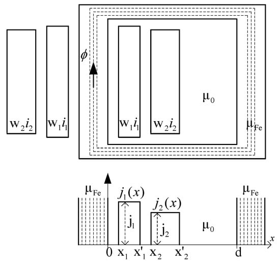
Figure 3.
Explanation of a 1D problem for a transformer’s air window.
In 1D, the magnetic field is described by the ordinary differential equation for the magnetic vector potential as follows:
This can be interpreted as two infinitely high windings located in the air between the ferromagnetic plates. The windings with currents have numbers of turns , respectively. Accounting for the ferromagnetic walls, the zero Dirichlet conditions can be stated on external points of the ferromagnetic walls. However, when omitting the ferromagnetic walls, assuming , it is difficult to formulate the boundary conditions at the points “0” and “d”. The zero Neumann conditions can be applied only in the case of balanced currents [24].
The difficulties can be better understood when interpreting Equation (7) as a thermal problem. Let us consider that there is one heating area only, with power density , instead of current density . The ferromagnetic walls should be interpreted as an ideal isolation. The temperature between such walls goes toward infinity, so the solution cannot be found. Considering the two balanced areas of heat: a positive source and a negative source, the zero Neumann conditions on the boundaries can be fulfilled. The solution describes the heat transfer between those two heat sources.
To account for the boundary conditions for non-balanced ampere-turns in the air window, the following numeric test has been carried out. The 1D problem for the case as in Figure 3 was solved using finite element method (FEM) software offered by FlexPDE by considering only excitation in winding “1”, and zero Dirichlet conditions at the outer boundaries of ferromagnetic zones. The permeability of ferromagnetic plates took four rising values , , and . Figure 4 shows the results: the ampere-turn function, the magnetic potential, and the magnetic field in the air zone. All magnetic potential starts in this figure from zero, but in fact their real values are given in Table 1. Those curves present magnetic potential on the level mentioned in Table 1. The numbers of colored lines correspond to the values of the ferromagnetic walls’ magnetic permeability.
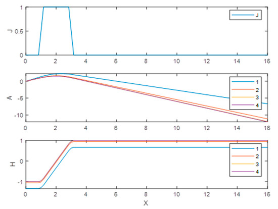
Figure 4.
Influence of the ferromagnetic walls’ magnetic permeability on the magnetic potential and the magnetic field in the air window.

Table 1.
Actual values of magnetic potential at x = 0.
Figure 5 presents the differences versus . It is rather evident that the difference stabilizes when the magnetic permeability of the ferromagnetic plates grows. However, most important is that the curve of the magnetic field changes at the boundaries to the opposite values, which differ proportionally to the ampere-turns of the winding. It means that the curve of magnetic potential has opposite derivatives at the air window boundaries. It seems to be an important indication of boundary conditions when magnetic field analysis is limited to the air zone only. In the case of one winding, the magnetic potential curve is composed of two straight lines in the air and of a parabolic curve in the area of the winding. Those straight lines have to have strictly the same but opposite derivatives, so the magnetic potential curve has its maximum exactly in the middle of the winding, i.e., the magnetic field takes the zero value at that point.
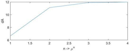
Figure 5.
Differences in magnetic potentials between boundaries of the air window versus
.
The method of images, presented in [25,26], can be used to solve the case of only one winding in the air zone. The interval of analysis is extended to . The ampere-turn function j(x) is composed in this new interval with two parts for and for , and the function fulfills the relation , as it is shown in Figure 6. The Fourier series of the function contain the odd harmonics only.
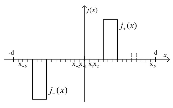
Figure 6.
Equivalent 1D problem of magnetic field calculation.
Equation (7), reduced to the air zone only, has the form
Its solution can also be predicted in the form of the Fourier series with odd harmonics only, and approximated by the series with terms, where R is an odd number of the highest harmonic:
Choosing a set of points regularly distributed in the interval (see Figure 6),
satisfying condition , the unique relations between values of the function and the Fourier coefficients can be established and written in a matrix form
where:
It allows us to find a modified discrete difference operator (DDO) of the second order , as presented in [25,26], binding the values of the second derivatives and the function itself at the chosen point set
where:
The application of this operator to Equation (8) leads to the finite-difference equation of the form
where:
Equation (12) determines the solution values at the point set . However, the following relation has to be satisfied
This allows us to reduce the finite-difference Equation (12) to the form
where and . The dimensions of those equations are reduced almost by half. The matrix of the operator still has one eigenvalue equal to zero, so Equation (14) can be solved assuming one arbitrary value, for instance .
Figure 7 compares the solution of Equation (14) to the FEM solution, for the same data. The curve marked as repeats the curve ‘4′ from Figure 4, whereas the curve presents the solution of Equation (14). The magnetic field curve was calculated from the formula , where is the first order DDO, corresponding to , which takes the form
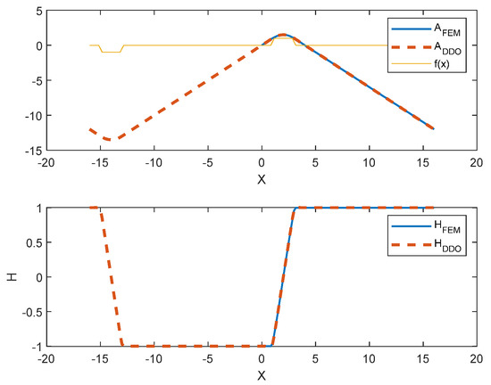
Figure 7.
Vector potential and magnetic field solutions of the finite element method (FEM) and discrete difference operator (DDO).
The solutions of FEM and DDO for vector potential and magnetic field practically overlap
The errors with regard to the FEM solution are:
- −
- for the magnetic vector potential
- −
- for the magnetic field
4. Calculations of Self- and Mutual Inductances Due to Fluxes in the Air Window for a 1D Approach
Magnetic field curves in the air zone can be rather easily drawn considering the results from the previous section. Figure 8 presents the magnetic field curves for the case shown in Figure 6. Successive curves present magnetic field distribution for three cases:
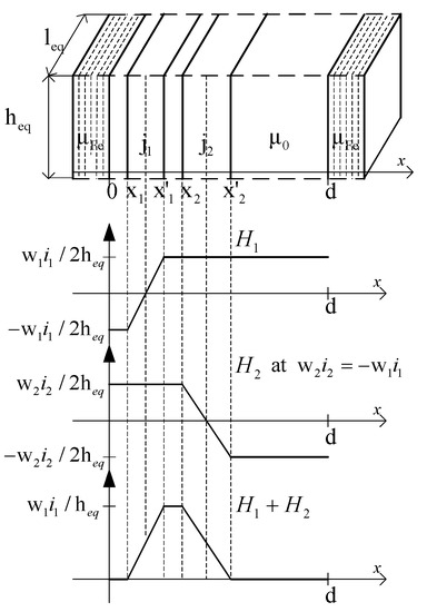
Figure 8.
Magnetic field distributions in the air zone for 1D approach.
- −
- generated by the winding ‘1′ with number of turns conducting the current
- −
- generated by the winding ‘2′ with number of turns conducting the current
- −
- generated by both windings at balanced ampere-turns .
The inductances can be calculated using the energy approach, i.e., determining the co-energy from Formula (5), which for the 1D field in the air reduces to the formula
where is an equivalent height and is an equivalent length of the air window. The inductance is determined from the formula
where .
The inductance is determined from the formula
where .
The mutual inductance fulfills the equation
where .
Finally, the leakages inductances are given by the formulae
and satisfy the relation
Those three inductances can be determined for any pair of independent windings located within one air window. This allows us to create the leakage inductance matrix in the relation (1). The short-circuit inductance follows from the Formula (4) and has the form
This is a well-known expression for the short-circuit inductance of two windings, which is valid if the 1D approach is acceptable for magnetic field analysis in the air window zone. It confirms the correctness of Formula (16) for the self- and mutual leakages inductances.
5. Conclusions
This paper presents very simple formulae for approximating self- and mutual leakage inductances of power transformer windings. They have been obtained using 1D calculations of magnetic field in an air zone only, applying discrete differential operators for periodic functions. The influence of the transformer’s ferromagnetic core on the magnetic field distribution in the air zone was initially analyzed with FEM.
Obtained formulae are valid if the 1D approach is acceptable for determining the magnetic field distribution in the transformer’s air window, i.e., when the Rogowski factor sufficiently corrects the length of the leakage flux in the air zone. Firstly, new formulae are applicable to multi-winding transformers with concentric windings more or less covering the transformer’s limbs. This improves the modelling of multi-winding transformers.
However, when the 1D approach is insufficient for transformers with windings located asymmetrically in the air window, the 2D problem of magnetic field distribution in the air window should be solved, but the boundary conditions for that problem should be stated. Until now, this problem has been solved in the cases of balanced ampere-turns in the air window at zero’s Neumann conditions on boundaries. This allows us to calculate the short-circuit inductances for individual pairs of windings only. The self- and mutual leakage inductances are calculated for such cases using 2D FEM by taking into account both the iron core and air zones.
Author Contributions
Conceptualization, T.S. and M.J.; methodology, T.S. and M.J.; software, M.J.; validation, T.S. and M.J.; formal analysis, T.S. and M.J.; investigation, T.S. and M.J.; resources, T.S.; data curation, T.S. and M.J.; writing—original draft preparation, T.S.; writing—review and editing, T.S. and M.J.; visualization, M.J.; supervision, T.S.; project administration, T.S.; funding acquisition, T.S. All authors have read and agreed to the published version of the manuscript.
Funding
This research, which was carried out under the theme Institute E-2, was funded by the subsidies on science granted by the Polish Ministry of Science and Higher Education.
Conflicts of Interest
The authors declare no conflict of interest.
References
- Jezierski, E. Transformers, Theoretical Background; WNT: Warsaw, Poland, 1965; pp. 103–149. (In Polish) [Google Scholar]
- Karsai, K.; Kerenyi, D.; Kiss, L. Large Power Transformers; Elsevier Publications: Amsterdam, The Netherlands, 1987. [Google Scholar]
- Winders, J.J., Jr. Power Transformers, Principles and Applications; Pub. Marcel Dekker, Inc.: New York, NY, USA, 2002. [Google Scholar]
- Del Vecchio, R.M.; Poulin, B.; Feghali, P.T.; Shah, D.M.; Ahuja, R. Transformers Design and Principles with Applications to Core-Form Power Transformers; Taylor & Francis: New York, NY, USA, 2002. [Google Scholar]
- Hurley, W.G.; Wölfle, W.H. Transformers and Inductors for Power Electronics: Theory, Design & Applications; John Wiley & Sons Pub.: Hoboken, NJ, USA, 2013. [Google Scholar]
- El Hayek, J. Short-circuit reactance of multi-secondaries concentric winding transformers. In Proceedings of the IEEE International Electric Machines and Drives Conference, Cambridge, MA, USA, 17–20 June 2001; MIT: Cambridge, MA, USA, 2001; pp. 462–465. [Google Scholar]
- El Hayek, J. Parameter Analysis of Multi-windings Traction Transformers. Ph.D. Thesis, Cracow University of Technology, Cracow, Poland, 2002. [Google Scholar]
- Chiver, O.; Neamt, L.; Horgos, M. Finite Elements Analysis of a Shell-Type Transformer. J. Electr. Electron. Eng. 2011, 4, 21. [Google Scholar]
- Ehsanifar, A.; Dehghani, M.; Allahbakhshi, M. Calculating the leakage inductance for transformer inter-turn fault detection using finite element method. In Proceedings of the 2017 Iranian Conference on Electrical Engineering (ICEE), Tehran, Iran, 2–4 May 2017. [Google Scholar] [CrossRef]
- Tsili, M.; Dikaiakos, C.; Kladas, A.; Georgilakis, P.; Souflaris, A.; Pitsilis, C.; Bakopoulos, J.; Paparigas, D. Advanced 3D numerical methods for power transformer analysis and design. In Proceedings of the 3rd Mediterranean Conference and Exhibition on Power Generation, Transmission, Distribution and Energy Conversion, MEDPOWER 2002, Athens, Greece, 4–6 November 2002. [Google Scholar]
- Hameed, K.R. Finite element calculation of leakage reactance in distribution transformer wound core type using energy method. J. Eng. Dev. 2012, 16, 297–320. [Google Scholar]
- Kaur, T.; Kaur, R. Modeling and Computation of Magnetic Leakage Field in Transformer Using Special Finite Elements. Int. J. Electron. Electr. Eng. 2016, 4, 231–234. [Google Scholar] [CrossRef][Green Version]
- Stnculescu, M.; Maricaru, M.; Hnil, F.I.; Marinescu, S.; Bandici, L. An iterative finite element - boundary element method for efficient magnetic field computation in transformers. Rev. Roum. Sci. Technol. 2011, 56, 267–276. [Google Scholar]
- Oliveira, L.M.R.; Cardoso, A.J.M. Leakage Inductances Calculation for Power Transformers Interturn Fault Studies. IEEE Trans. Power Deliv. 2015, 30, 1213–1220. [Google Scholar] [CrossRef]
- Jahromi, A.; Faiz, J.; Mohseni, H. Calculation of distribution transformer leakage reactance using energy technique. J. Fac. Eng. 2004, 38, 395–403. [Google Scholar]
- Jahromi, A.; Faiz, J.; Mohseni, H. A fast method for calculation of transformers leakage reactance using energy technique. IJE Trans. B Appl. 2003, 16, 41–48. [Google Scholar]
- Dawood, K.; Alboyaci, B.; Cinar, M.A.; Sonmez, O. A New method for the Calculation of Leakage Reactance in Power Transformers. J. Electr. Eng. Technol. 2017, 12, 1883–1890. [Google Scholar] [CrossRef]
- Dawood, K.; Cinar, M.A.; Alboyaci, B.; Sonmez, O. Calculation of the leakage reactance in distribution transformers via numerical and analytical methods. J. Electr. Syst. 2019, 15, 213–221. [Google Scholar]
- Guemes-Alonso, J.A. A new method for calculating of leakage reactances and iron losses in transformers. In Proceedings of the Fifth International Conference on Electrical Machines and Systems (IEEE Cat. No.01EX501), Shenyang, China, 18–20 August 2001; Volume 1, pp. 178–181. [Google Scholar] [CrossRef]
- Schlesinger, R.; Biela, J. Comparison of Analytical Models of Transformer Leakage Inductance: Accuracy Versus Computational Effort. IEEE T. POWER SYST. 2002, 36, 146–156. [Google Scholar] [CrossRef]
- Wachta, B. Calculation of Leakages in Unsymmetrical Multi-Windings Transformers; Scientific Bull.; Univ. of Mining & Metallurgy: Kraków, Poland, 1969; pp. 7–27. (In Polish) [Google Scholar]
- Jamali, S.; Ardebili, M.; Abbaszadeh, K. Calculation of short circuit reactance and electromagnetic forces in three phase transformers by finite element method. In Proceedings of the 8th International Conference Electrical Machines & Systems, Nanjing, China, 27–29 September 2005; Volume 3, pp. 1725–1730. [Google Scholar]
- El Hayek, J.; Sobczyk, T.J. Multi-port equivalent scheme for multi-winding traction transformers. COMPEL 2012, 31, 726–737. [Google Scholar] [CrossRef]
- Sobczyk, T.J.; El Hayek, J. On parameters determination of multi-port equivalent circuit for multi-windings traction transformers. Arch. Electr. Eng. Pol. Acad. Sci. 2015, 64, 17–28. [Google Scholar]
- Jaraczewski, M.; Sobczyk, T.J. Numerical tests of novel finite difference operator for solving 1D boundary-value problems. In Proceedings of the 2019 15th Selected Issues of Electrical Engineering and Electronics (WZEE), Zakopane, Poland, 8–10 December 2019. [Google Scholar]
- Sobczyk, T.J.; Jaraczewski, M. Application of Discrete Differential Operators of Periodic Function to Solve 1D Boundary Value Problems, COMPEL-The International Journal for Computation and Mathematics in Electrical and Electronic Engineering; Emerald Pub. Ltd.: London, UK, 2020; pp. 885–897. [Google Scholar] [CrossRef]


© 2020 by the authors. Licensee MDPI, Basel, Switzerland. This article is an open access article distributed under the terms and conditions of the Creative Commons Attribution (CC BY) license (http://creativecommons.org/licenses/by/4.0/).