Article

Performance Evaluation of Analytical Methods for Parameters Extraction of Photovoltaic Generators

1
School of Engineering, University of Wolverhampton, Telford TF2 9NT, UK
2
Department of Electrical Technique, Southern Technical University, Technical Institute-Qurna, Basra, Iraq
*
Author to whom correspondence should be addressed.
Energies 2020, 13(18), 4825; https://doi.org/10.3390/en13184825
Submission received: 21 August 2020 / Revised: 10 September 2020 / Accepted: 14 September 2020 / Published: 15 September 2020
(This article belongs to the Collection Renewable Energy and Energy Storage Systems)

Abstract

:
This paper presents a succinct exploration of several analytical methods for extracting the parameters of the single-diode model (SDM) of a photovoltaic (PV) module under standard test conditions (STC). The paper investigates six methods and presents the detailed mathematical analysis leading to the development of each method. To evaluate the performance of these methods, MATLAB-based software has been devised and deployed to generate the results of each method when used to extract the SDM parameters of various PV test modules of different PV technologies. Similar software has also been developed to extract the same parameters using well-established numerical and iterative techniques. A comparison is subsequently made between the synthesized results and those obtained using numerical and iterative methods. The comparison indicates that although analytical methods may involve a significant amount of approximations, their accuracy can be comparable to that of their numerical and iterative counterparts, with the added advantage of a significant reduction in computational complexity, and without the initialization and convergence difficulties, which are normally associated with numerical methods.

1. Introduction

Photovoltaic (PV) systems offer the most direct conversion of the sunlight energy into electricity making them one of the most appealing systems for renewable energy generation [1]. The principle component of a PV power plant is the PV generator, which typically consists of an array of PV modules connected in series and or parallel combinations to provide the terminal voltage and current required to furnish the rated power of the plant. To harness the harvested solar energy and convert it into a useable form of electricity for the end user, a PV plant uses different types of power electronic systems, such as DC–DC and DC–AC converters [2]. The design, analysis and simulation of a PV system including these power converters, require a lumped-parameter equivalent circuit model of the PV generator. Such an equivalent circuit is used for purposes, such as efficient sizing of the PV array and of the semiconductor switching devices of the power converters. In addition, it can be used with circuit simulation software packages.
The normalized current–voltage (I–V) and power–voltage (P–V) characteristics of a typical PV generator are shown in Figure 1. The general shapes of these characteristics are similar regardless of the size of the PV generator, i.e., be it a cell, a module, or an array of modules. These curves reveal three important salient points: the open-circuit (OC) voltage, the short-circuit (SC) current, and the maximum power point (MPP). For maximum power extraction from any PV generator, the generator must be continuously operated at its MPP (maximum power point). However, the load is normally variable, which implies that the load-line will not necessarily coincide with the MPP. Moreover, the terminal characteristics of a photovoltaic generator vary with climatic conditions of temperature and insolation thus, the MPP will also change with variations in insolation and temperature [3,4]. Hence, to maintain operation at the current MPP, a photovoltaic system utilises an MPPT (maximum power point tracker) system that forces the operating point of a PV generator to continuously follow the prevailing MPP regardless of variations in the load and or environmental conditions [5].
An MPPT system uses a DC–DC power converter controlled by an MPPT algorithm that is normally implemented using a microcontroller [6]. The design of an MPPT system is made more difficult due to the effects of PS (partial shading) [7]. Partial shading can lead to significant reduction in the energy yield of a PV system and its reliability [8,9]. To mitigate the adverse consequences of PS, bypass diodes are normally deployed in PV modules [10] and arrays [11]. However, these diodes can give rise to power–voltage curves with multiplicity of power peaks which complicates the design of the MPPT system [5]. Therefore, an equivalent circuit model of a PV generator is also required to aid the design and simulation of the MPPT system, to investigate the adverse effects of PS and explore strategies of mitigating them [12]. The single-diode model (SDM) of a PV generator, is currently the dominant lumped-parameter equivalent circuit model, due to its accuracy and reduced complexity [13,14,15]. Furthermore, it can be readily modified to model a PV generator of any size [2,16].
As shown in Figure 2, the SDM includes five parameters which must be estimated: The saturation current I s a t and the ideality factor n of the diode, the series resistance R s , the shunt resistance R s h , and the photocurrent I p h [13]. These five model parameters are not provided in datasheets of PV modules, but can be estimated, or extracted, from information provided in datasheets. However, information given in a datasheet of a PV module is specified under only one operating condition, namely the standard test conditions (STC) (insolation G = 1000   W / m 2 , temperature T = 25   ° C , and Air mass AM = 1.5) thus, the extracted parameters are only valid at STC. For any other arbitrary conditions of insolation and temperature, these STC parameters must be adapted accordingly [4,17].
To estimate the model parameters of the SDM at STC, numerous methods with varying degrees of mathematical and computational complexities and accuracy have been reported in the literature, for example [14,18,19]. These methods are commonly classified as either analytical or numerical. Numerical, or explicit methods, generate a system of equations which can be solved using numerical/iterative algorithms such as the Newton–Raphson solution strategy. The disadvantages of numerical methods include the need for appropriate initialisation, can produce trivial solutions, and may have convergence difficulties. Analytical methods on the other hand, use simple and fast parameter extraction schemes by making use of some simplifying assumptions and approximations [20]. For example, by disregarding some parameters or allocating some approximate values for some other parameters as detailed in Section 3 [21,22].
In addition, there are other strategies for the parameter extraction, such as those based on computational intelligence [23] and those using meta-heuristic algorithms [24]. More complex methods of parameter extraction can also be found in the literature, such as those based on optimisation algorithms [25,26] and those based on differential evolution [27]. There are also analytical methods which are based on the double-diode circuit model which has seven parameters [28,29]. However, the scope of this article is restricted to analytical methods which use the universally adopted SDM of a PV module.
Referring to the SDM in Figure 2, the terminal current I of a PV module consisting of N s PV cells connected in series, is given by the general current equation:
I = I p h I s a t [ exp ( V + I R s n N s V t h ) 1 ] V + I R s R s h
The first term is the photocurrent I p h which is almost directly proportional to the incident insolation. The second term, in the above equation, is the Shockley’s equation, which represents the diode current I d , while the third term is the current in the shunt resistance I s h . The diode’s thermal voltage V t h is defined in terms of the electronic charge q = 1.602 × 10 19   C , the Boltzmann’s constant k = 1.38065 × 10 23   J / K and temperature T (K) as:
V t h = k T q
At room temperature, the thermal voltage is about 26 mV. The ideality factor for a silicon PV cell is typically between one and two. For a typical PV module, the series resistance is in the order of 1 Ω, the parallel resistance is in the region of few hundred ohms, and the saturation current is in the order of nano-Amperes.
Equation (1) is an implicit and transcendental equation that would normally require a numerical solution to obtain the five parameters of the SDM. However, since numerical methods are susceptible to convergence and initialisation difficulties, several alternative analytical methods have been described in the literature. These methods aim at reducing the complexity of the implicit general equation of the SDM by introducing some approximations to develop explicit models as detailed in Section 3. For example, some methods use the approximation that the shunt resistance is the reciprocal of the gradient of the I–V characteristic curve under short-circuit condition [20]. Others neglect the shunt resistance on the assumption that it is relatively too large [30], while some analytical methods neglect both the series and the shunt resistances [22].
The contributions of this article are: Explore the most literature-reported analytical methods for parameters extraction of the SDM, present detailed derivation of the mathematical expressions that lead to each method which are not normally detailed in the reporting literature, and synthesize the results of each method by deploying them to extract the parameters of PV modules of different technologies. Finally, the paper presents a comparison between these synthesized results and those obtained using numerical and iterative techniques.
After this introductory section, Section 2, describes mathematical analysis that supports the development of the analytical methods investigated in this work. Section 3 presents detailed mathematical derivation and formulation of the expressions required for extracting each parameter using each method. Section 4 provides a discussion of the results and finally, Section 5 summarises the main findings of the work presented in this article.

2. Mathematical Grounds for the Analytical Methods

When the entire I–V curve is available, the parameters of the SDM may be estimated using curve fitting or optimisation algorithm [26,31,32]. In general, the I–V characteristics are not given in manufacturers’ datasheets and even when provided, they are specified under only one operating condition, namely the STC [33]. Most methods used to extract the SDM parameters are based on developing the model equations using data at the three salient points (SC, OC, MPP), which are always provided in the datasheet of a photovoltaic module. There are three standard equations used in most studies, e.g., in [14,18,21], which are derived from Equation (1) at the three salient points: ( 0 , I s c ), ( V o c , 0 ), and ( V m p , I m p ) under STC as explained next.
Substituting the SC point ( 0 , I s c ), in Equation (1), we arrive at the SC equation as:
I s c = I p h I s a t [ exp ( I s c R s n N s V t h ) 1 ] I s c R s R s h
Similarly, substituting the OC point V o c , 0 in Equation (1) and rearranging, we obtain the OC equation as:
I p h = I s a t [ exp ( V o c n N s V t h ) 1 ] + V o c R s h
Substituting the maximum power point V m p , I m p in Equation (1), we obtain the MPP equation as:
I m p = I p h I s a t [ exp ( V m p + I m p R s n N s V t h ) 1 ] V m p + I m p R s R s h
Another important quantity required for parameter extraction is the derivative of the module’s current with respect to its voltage, i.e., d I / d V . This is obtained by differentiating Equation (1):
d I d V = I s a t n N s V t h [ exp ( V + I R s n N s V t h ) ( 1 + d I d V R s ) ] [ 1 R s h + d I d V R s R s h ]
Solving for the derivative:
d I d V = I s a t n N s V t h [ exp ( V + I R s n N s V t h ) ] 1 R s h ( 1 + R s R s h + I s a t R s n N s V t h exp ( V + I R s n N s V t h )
It is to be noted that the above expression for the derivative is valid at any point on the I–V curve. Another derivative used in parameter extraction procedures is that of the power with respect to voltage defined as:
d P d V = d d V ( V I ) = V I V + I V V
At the MPP point, this derivative equates to zero:
d P d V MPP = 0 = V m p I V + I m p V V
Therefore, at the MPP the current derivative becomes:
d I d V MPP = I m p V m p
The shunt resistance at the SC point R s h o , may be estimated from the gradient of the I–V curve at the short-circuit point as:
d I d V SC = 1 R s h o
Similarly, the series resistance at the OC point R s o is defined as:
d I d V OC = 1 R s o
For the five parameters extraction process, the majority of the parameter extraction methods, for example [14,19,22,34,35,36,37,38], have taken into account the mathematical correlation between these parameters and separated them into two levels: The main level consists of the ideality factor, shunt resistance, series resistance, and a secondary level which consists of the photocurrent and the saturation current. This way, the extraction equations are reduced to three instead of five to simplify the mathematical formulation as illustrated in the next section.

3. Parameters Extraction Methods

In this section we present the mathematical analysis and derivation of the equations required for the extraction of the SDM parameters for six main analytical methods.

3.1. Method One

This method was developed to determine the parameters of a blue and grey solar cell using experimentally obtained I–V curve and the three salient points, i.e., the SC, OC, and the MPP, which are available in datasheets [20]. The method uses several approximations to simplify the required extraction equations and is based on calculating a value of the ideality factor, n, as the main model parameter, which is consequently used to estimate the remaining four parameters, namely R s , R s h , I p h , and I s a t . As explained in the following subsections, the method uses Equations (3)–(5), (11) and (12) to extract the model parameters with the term N s set to unity since the method was described for a single PV cell as opposed to a PV module.

3.1.1. Extraction of the Photocurrent

The photocurrent is estimated using the short-circuit current point 0 , I s c , i.e., Equation (3), which we can be re-arrange to obtain an expression for the photocurrent as:
I p h = I s c ( 1 + R s R s h ) + I s a t [ exp ( I s c R s n V t h ) 1 ]
The short-circuit current I s c is obtained from the datasheet. However, R s , R s h , and I s a t are unknowns and must be determined.

3.1.2. Extraction of the Shunt Resistance

We can derive an expression to estimate the shunt resistance using the expression for derivative d I / d V expressed at the short-circuit point. Substituting the short-circuit point ( 0 , I s c ) in the expression of the derivative of Equation (7), and setting N s = 1 , we obtain:
d I d V S C ( 1 + R s R s h + I s a t R s n V t h exp ( I s c R s n V t h ) = I s a t n V t h [ exp ( I s c R s n V t h ) ] + 1 R s h
Substituting for the derivative at the SC point from Equation (11) into Equation (14) we obtain:
R s h o I s a t n V t h [ exp ( I s c R s n V t h ) + 1 R s h = ( 1 + R s R s h + I s a t R s n V t h exp ( I s c R s n V t h )
The exponential term [ I s a t exp ( I s c R s / n V t h ) ] represents the diode current under short-circuit condition, which is too small compared to the short-circuit current hence, it may be neglected [39]. Further, since R s R s h , the term R s / R s h may also be neglected. Therefore, Equation (15) becomes:
R s h = R s h o
This means that the shunt resistance is estimated directly from the gradient of the I–V curve at the SC point.

3.1.3. Extraction of the Series Resistance

To estimate the series resistance, we can use the gradient of the I–V curve at the OC voltage point. Substituting the OC point ( V o c , 0 ) and setting N s = 1 in the general expression for the derivative of Equation (7), we can write:
d I d V OC ( 1 + R s R s h + I s a t R s n V t h exp ( V o c n V t h ) = I s a t n V t h [ exp ( V o c n V t h ) ] + 1 R s h
Substituting for the derivative at the OC point from Equation (12) and re-arranging:
R s o I s a t n V t h [ exp ( V o c n V t h ) ] + 1 R s h = ( 1 + R s R s h + I s a t R s n V t h exp ( V o c n V t h )
The term I s a t exp V o c / n V t h represents the diode current under open-circuit condition. Under this condition, the diode current is the photocurrent, which is the same as the SC current less the negligibly small current in the shunt resistance. When this diode current is divided by n V t h the result is much greater than 1 / R s h thus, the latter term can be neglected. Further, after neglecting the term R s / R s h , the expression for series resistance becomes:
R s = R s o n V t h I s a t exp ( V o c n V t h )
This is not a closed form expression for the series resistance since it contains the saturation current and the ideality factor which need to be determined. The open-circuit voltage is obtained from the datasheet.

3.1.4. Extraction of the Reverse Saturation Current

By substituting, the open-circuit Equation (4) into the short-circuit Equation (3) and neglecting the (−1) in the exponential terms, we obtain:
I s c = I s a t [ exp ( V o c n V t h ) exp ( I s c R s n V t h ) ] + V o c R s h I s c R s R s h
This may be re-arranged as:
I s a t [ exp ( V o c n V t h ) exp ( I s c R s n V t h ) ] ( R s R s h + 1 ) I s c + V o c R s h = 0
However, since in practice at I s c R s V o c and R s R s h [39,40], the equation for the saturation current becomes:
I s a t = I s c V o c R s h exp V o c n V t h
The OC voltage and the parallel resistance can be estimated from the I–V curve however, the ideality factor is still unknown and needs to be determined.

3.1.5. Extraction of the Ideality Factor n

Substituting the OC voltage equation for the photocurrent, i.e., Equation (4), into the MPP Equation (5), and after ignoring the (−1) in the exponential terms, we can write:
I s a t exp ( V o c n V t h ) I s a t exp ( V m p + I m p R s n V t h ) + V o c V m p R s h I m p ( 1 + R s R s h ) = 0
Since R s R s h , this reduces to:
I s a t exp ( V o c n V t h ) I s a t exp ( V m p + I m p R s n V t h ) + V o c V m p R s h I m p = 0
An expression for the ideality factor can now be derived as explained below.
Substituting Equation (16) into (22):
I s a t = I s c V o c R s h o exp V o c n V t h
Substituting Equation (25) into (24), we obtain:
I s c V o c R s h o exp V o c n V t h exp V o c n V t h I s c V o c R s h o exp V o c n V t h exp ( V m p + I m p R s n V t h ) + V o c V m p R s h o I m p = 0
This can be simplified to:
V m p + I m p R s V o c n V t h = ln I s c I m p V m p R s h o ln I s c V o c R s h o
Therefore, the ideality factor becomes:
n = V m p + I m p R s V o c V t h ln I s c I m p V m p R s h o ln I s c V o c R s h o
This is not a closed from expression because it contains the series resistance, which must be determined. This can be obtained by substituting the expression for the saturation current of Equation (25) into the expression for the series resistance of Equation (19) as:
R s = R s o n V t h I s c V o c R s h o exp V o c n V t h exp V o c n V t h
Hence, the expression for the series resistance becomes:
R s = R s o n V t h I s c V o c R s h o
Substituting this expression for the series resistance, i.e., Equation (30), into Equation (28):
n = V m p V o c + I m p R s o n V t h ( I s c V o c / R s h o ) V t h ln I s c I m p V m p R s h o ln I s c V o c R s h o
This can be simplified to:
n V t h ln V m p R s h o + I s c I m p ln I s c V o c R s h o + I m p ( I s c V o c / R s h o ) = V m p V o c + I m p R s o
Solving for the ideality factor:
n = V m p V o c + I m p R s o V t h ln V m p R s h o + I s c I m p ln I s c V o c R s h o + I m p ( I s c V o c / R s h o )
This is now a closed form expression for the ideality factor because all the variables can be obtained or estimated from the datasheet and the I–V curve of the cell. For a PV module with N s cells connected in series, the ideality factor is multiplied by N s [2]. Having estimated the ideality factor, the saturation current can then be estimated using Equation (25) and consequently, the series resistance obtained from (19). Finally, the photocurrent can be calculated using (13). The major deficiency of this method is the fact that it requires the I–V curve, which is not always available in the manufacturer’s datasheet.

3.2. Method Two

This method uses the idealised SDM model shown in Figure 3, which neglects the effects of the both, the series and shunt resistances. The method results in simplified analytical expressions for current, voltage, and power [22].
The general current equation for this model is:
I = I p h I s a t exp ( V n N s V t h ) 1
A the short-circuit point 0 , I s c , this reduces to:
I p h = I s c
That is the photocurrent is the same as the SC current, and this is always provided by the PV module’s datasheet. At the open-circuit point V o c , 0 , we have:
I p h = I s a t ( exp ( V o c n N s V t ) 1 )
Alternatively, since in this model, I s c = I p h , we may write:
I s c = I s a t [ exp ( V o c n N s V t ) 1 ]
We can solve this for the OC voltage as:
V o c = n N s V t h ln I s c I s a t + 1
Using Equation (37), the saturation current can be expressed as:
I s a t = I s c exp ( V o c n N s V t h ) 1
At the MPP, we can express the current as:
I m p = I s c I s a t exp ( V m p n N s V t h ) 1
The derivative d I / d V at any point along the I–V curve can be obtained from Equation (34) as:
d I d V = I s a t n N s V t h exp ( V n N s V t h )
The derivative at the maximum power point is:
d I d V MPP = I m p V m p
Substituting Equation (42) into Equation (41), the current at the MPP becomes:
I m p = V m p I s a t n N s V t h exp ( V m p n N s V t h )
Substituting (37) and (43) into (40) and ignoring the (−1) in the exponential terms:
[ exp ( V o c n N s V t ) ] = exp ( V m p n N s V t h ) ( 1 + V m p n N s V t h )
Equations (35), (38), (43) and (44) represent the main equations of the explicit model. To estimate the maximum power point voltage V m p , the derivative in Equation (41) at the MPP is solved for the MPP voltage as:
V m p = n N s V t h ln n N s V t h I s a t d I d V V m p
The asymptotic behaviour of the I–V curve around the open-circuit and short-circuit points were used to estimate the derivative needed in the above equation as [22]:
d I d V M p p Δ I Δ V = 0 I s c V o c 0 = I s c V o c
Substituting Equation (46) into (45), we obtain:
V m p = n N s V t h ln n N s V t h I s a t I s c V o c
Substituting Equation (47) into (40):
I m p = I s c I s a t exp [ n N s V t h ln n N s V t h I s a t I s c V o c n N s V t h ] 1
Simplifying the above, we obtain:
I m p = I s c + I s a t I s a t n N s V t h I s a t I s c V o c
I m p = I s c + I s a t n N s V t h I s c V o c
The maximum power is:
P m = V m p I m p
Therefore,
P m = n N s V t h ( I s c + I s a t   n N s V t h I s c V o c )   ln n N s V t h I s a t ( I s c V o c )
To estimate the ideality factor under STC conditions, we substitute Equation (39) into (40) and ignore the (−1) since the exponential terms in both is much larger than unity:
I m p = I s c I s c exp ( V o c n N s V t ) exp ( V m p n N s V t h )
Re-arranging and simplifying, we obtain:
n N s V t h ln 1 I m p I s c = ( V m p V o c )
Solving for the ideality factor at STC, we obtain:
n = V m p V o c N s V t h ln 1 I m p I s c
In attempting to improve the accuracy of this method, Mahmoud et al. [41] modified the saturation current equation as:
I s a t = exp ( β Δ T q   G [ I s c + α Δ T ] n N s k T ) ( G I s c / I s a t , S C T + 1 ) T S T C T exp ( β Δ T q   G n N s k T )
where Δ T = T T S T C and β is the voltage temperature coefficient, which is always included in the datasheet. The STC saturation current can be computed as [14]:
I s a t , S T C = I s c [ exp ( V o c / n N s V t h ) 1 ]
Yousef et al. [42] improved the accuracy of the ideal model of the PV module at low irradiance without affecting the simplicity of the model by modifying the equation of the saturation current to take into account the effect of the low irradiance on the OC voltage as:
I s a t = I p h ( G , T ) [ exp q ( V o c β Δ T + Δ V o c ( G 1 , T S T C ) ) 1 ]
V o c = n N s k T q ln ( I p h I s a t + 1 )
Δ V o c ( G , T S T C ) = n N s k T q ln ( G G S T C )

3.3. Method Three

This method assumes that the shunt resistance is very large so that it can be neglected hence, it is developed using the single-diode equivalent circuit model shown in Figure 4. This model, which is known as the four parameters model, has been found to offer good accuracy [30,43]. The method uses the datasheet, but does not require the full I–V curve [30,43,44,45] which is not normally available. The model equations can be derived as illustrated below. The general current equation for this model is:
I = I p h I s a t [ exp ( V + I R s n N s V t h ) 1 ]
The short-circuit equation is:
I s c = I p h I s a t [ exp ( I s c R s n N s V t h ) 1 ]
The open-circuit equation is:
0 = I p h I s a t [ exp ( V o c n N s V t h ) 1 ]
The MPP equation is:
I m p = I p h I s a t [ exp ( V m p + I m p R s n N s V t h ) 1 ]

3.3.1. Extraction of the Photocurrent

Referring to the equation of the short-circuit condition, i.e., Equation (62), the second term represents the diode current. In practice, since the voltage I s c R s is too small and comparable to the thermal voltage, the exponential term exp ( I s c R s / n N s V t h ) is close to unity. Further, since this is multiplied by the very small value of the saturation current, it is reasonable to assume that the under short-circuit condition, the diode current is much smaller than the short-circuit current and can be neglected, i.e., all of the photocurrent is the SC current, hence Equation (62) reduces to:
I p h = I s c
That is the module’s photocurrent is the same as the SC current, which is always given in datasheets.

3.3.2. Extraction of the Saturation Current

Under open-circuit condition, the entire short-circuit current is the diode current, i.e.,
I s c = I s a t [ exp ( V o c n N s V t h ) 1 ]
Since the exponential term is much greater than one, we can ignore the (−1) hence, the saturation current can be expressed as:
I s a t = I s c [ exp ( V o c n N s V t h ) ]
This is, however, not a closed form expression for the saturation current since it includes the ideality factor which must be determined.

3.3.3. Extraction of the Series Resistance

The series resistance may be found by substituting Equation (67) into the MPP Equation (64) as:
I m p = I p h I s c [ exp ( V o c n N s V t h ) ] [ exp ( V m p + I m p R s n N s V t h ) 1 ]
Neglecting the (−1) in the second exponential term and replacing the photocurrent by the short-circuit current and re-arranging:
1 I m p I s c = [ exp ( V o c n N s V t h ) ] [ exp ( V m p + I m p R s n N s V t h ) ]
Re-arranging and solving for the series resistance, we obtain:
R s = n N s V t h ln ( 1 I m p I s c ) + V o c V m p I m p
This is not a closed form expression since it includes the ideality factor, which needs to be determined.

3.3.4. Extraction of the Ideality Factor

The ideality factor is derived using the fact that the slope of the I–V curve at the maximum power point is equal to zero. Equating Equation (10) and Equation (7) at the MPP:
I m p V m p = I s a t n N s V t h [ exp ( V m p + I m p R s n N s V t h ) ] ( 1 + I s a t R s n N s V t h exp ( V m p + I m p R s n N s V t h )
Re-arranging as:
V m p I m p = 1 I s a t n N s V t h [ exp ( V m p + I m p R s n N s V t h ) ] + R s
The above may be written as:
R s V m p I m p = n N s V t h I s a t [ exp ( V m p + I m p R s n N s V t h ) ]
Substituting for the series resistance R s from (70) into (73) we obtain:
n N s V t h ln ( 1 I m p I s c ) + V o c 2 V m p I m p = n N s V t h I s a t [ exp ( V m p + I m p R s n N s V t h ) ]
This may be re-arranged as:
ln ( 1 I m p / I s c ) I m p + ( 2 V m p V o c ) / n N s V t h I m p = 1 I s a t [ exp ( V m p + I m p R s n N s V t h ) ]
Substituting for the saturation current from Equation (67):
ln ( 1 I m p / I s c ) I m p + ( 2 V m p V o c ) / n N s V t h I m p = 1 I s c [ exp ( V o c n N s V t h ) ] [ exp ( V m p + I m p R s n N s V t h ) ]
This may be re-arranged as:
ln ( 1 I m p / I s c ) I m p + ( 2 V m p V o c ) / n N s V t h I m p = 1 I s c [ exp ( V m p + I m p R s V o c n N s V t h ) ]
The denominator on the right-hand side of Equation (77) may be re-written with the series resistance substituted by its expression from Equation (70) and simplified as follows:
I s c [ exp ( V m p + I m p R s V o c n N s V t h ) ] = I s c exp [ V m p V o c + I m p ( n N s V t h ln ( 1 I m p I s c ) + V o c V m p I m p ) n N s V t h ]
Re-arranging:
I s c [ exp ( V m p + I m p R s V o c n N s V t h ) ] = I s c exp [ ln ( 1 I m p I s c ) ]
Therefore:
I s c [ exp ( V m p + I m p R s V o c n N s V t h ) ] = I s c I m p
Substituting (80) into (77)
ln ( 1 I m p / I s c ) I m p + ( 2 V m p V o c ) / n N s V t h I m p = 1 I s c I m p
Simplifying and solving for the ideality factor:
n = ( 2 V m p V o c ) N s V t h [ I m p I s c I m p + ln ( 1 I m p I s c ) ]
This is a closed form expression for the ideality factor since all variables in its expression are available in the datasheet. Therefore, R s and I s a t can now be determined.

3.4. Method Four

This method uses information available in the datasheet to estimate the parameters of the SDM. It uses a piecewise I–V curve fitting scheme along with the four parameters PV model to evaluate them [45]. In this method the definition of the modified ideality factor is introduced as:
a = n N s V t h
Using Equation (7) the derivative of voltage with respect to current d V / d I is:
d V d I = R s ( 1 R s h + I s a t a exp ( V + I R s a ) + 1 I s a t a [ exp ( V + I R s a ) ] + 1 R s h
Simplifying:
d V d I = R s a R s h a + I s a t R s h exp ( V + I R s a )
At the SC point, the derivative becomes:
d V d I SC = R s a R s h a + I s a t R s h exp ( I s c R s a )
At the OC point, the derivative becomes:
d V d I OC = R s a R s h a + I s a t R s h exp ( V o c a )
At the MPP point, the derivative is:
d V d I MPP = R s a R s h a + I s a t R s h exp ( V m p + I m p R s a )
Equating equations (88) with the reciprocal of the derivative defined in Equation (10):
V m I m = R s + a R s h a + I s a t R s h exp ( V m p + I m p R s a )
Using Equations (3), (4), (87), (88) and (89) with a series of simplifications, the following equations are obtained to extract the five parameters R s , R s h , I p h , a , and the saturation current I s a t [45]:
R s = V m p ( d V d I O C d V d I S C ) d V d I S C ( I s c I m p ) + V m p d V d I O C ( d V d I S C I m p + V m p ) ( d V d I S C I s c + V o c ) I m p ( d V d I O C d V d I S C ) [ d V d I S C ( I s c I m p ) + V m p ] + ( d V d I S C I m p + V m p ) ( d V d I S C I s c + V o c )
R s h = R s d V d I SC
I p h = I s c ( 1 + R s R s h )
a = ( d V d I OC + R s ) ( d V d I s c I s c + V o c ) d V d I O C d V d I s c
And
I s a t = ( I p h V o c R s h ) / ( exp ( V o c / a ) 1 )
According to the actual measurement of a PV module, the I–V curve in the low- and high-voltage zones is smooth and can be represented by straight lines therefore, the slopes of the straight lines can be considered as the differential values of the I–V curve in the two zones as explained in [46], that is:
d V d I = Δ V Δ I

3.5. Method Five

This method which is also based on the manufacturer’s datasheet, uses a reduced set of approximations compared to the previous analytical methods without increasing complexity by incorporating two boundary conditions [40]. The first boundary condition is the derivative of the power with respect to voltage, which is used to derive expressions for the series and shunt resistances. The second condition is the slope at short-circuit point, which is used to estimate a value for the ideality factor. Both boundary conditions contributed significantly to improving the accuracy of the parameter extraction process [40].
Referring to Equation (3), the term [ exp ( I s c R s / n V t h ) ] is very close to unity and hence, the diode current is very small when compared with either the SC current or the shunt resistance current and hence, may be neglected [39,47,48]. This leads to:
I s c = I p h I s c R s R s h
Therefore, we can write for the photocurrent:
I p h = I s c R s + R s h R s h
Substituting (97) in Equation (4), and neglecting the (−1) in the exponential term of the latter, we have:
I s c R s + R s h R s h = I s a t [ exp ( V o c n N s V t h ) ] + V o c R s h
Solving for the saturation current:
I s a t = I s c ( R s + R s h ) V o c R s h exp ( V o c n N s V t h )
Substituting equations (97) and (99) into Equation (5) and ignoring the (−1) in the exponential term in the latter:
I m p = I s c R s + R s h R s h I s c ( R s + R s h ) V o c R s h exp ( V o c n N s V t h ) [ exp ( V m p + I m p R s n N s V t h ) ] V m p + I m p R s R s h
Simplifying:
I m p = I s c R s + I s c R s h V m p I m p R s R s h I s c R s + I s c R s h V o c R s h exp ( V m p + I m p R s V o c n N s V t h ) ]
This may be re-arranged as:
I m p = ( I s c V m p + I m p R s I s c R s R s h ) ( I s c V o c I s c R s ) R s h ) [ exp ( V m p + I m p R s V o c n N s V t h ) ]
Considering the equation for the derivative, Equation (6), at the MPP and using Equation (10), we can write:
I m p V m p = I s a t n N s V t h 1 I m p V m p R s exp ( V m p + I m p R s n N s V t h ) + 1 R s h I m p V m p R s R s h
Substituting (97), (99) and (102) in (103):
I m p V m p = 1 n N s V t h I s c ( R s + R s h ) V o c R s h ( 1 I m p V m p R s ) exp ( V m p + I m p R s V o c n N s V t h ) + 1 R s h I m p V m p R s R s h
Using equations (97) and (102), we can re-write Equation (104) as:
I m p + V m p 1 R s h I s c R s h V o c + I s c R s n N s V t R s h exp V m p + I m p R s V o c n N s V t 1 + R s R s h + I s c R s h V o c + I s c R s n N s V t R s h R s exp V m p + I m p R s V o c n N s V t = 0
From Equation (105), an expression for the shunt resistance may be obtained as follows:
I m p 1 + R s R s h + ( I s c R s h V o c + I s c R s n N s V t R s h ) R s exp V m p + I m p R s V o c n N s V t V m p 1 R s h I s c R s h V o c + I s c R s n N s V t R s h exp V m p + I m p R s V o c n N s V t = 0
Multiplying Equation (106) by R s h and re-arranging:
R s h I m p + I m p R s + I m p ( I s c R s h V o c + I s c R s ) R s n N s V t exp V m p + I m p R s V o c n N s V t V m p V m p ( I s c R s h V o c + I s c R s ) n N s V t exp ( V m p + I m p R s V o c n N s V t = 0
Let x be defined as:
x = V m p + I m p R s V o c n N s V t
Hence, (107) becomes:
R s h I m p + I m p R s + I s c R s h n N s V t I m p R s exp ( x ) + ( V o c + I s c R s ) n N s V t I m p R s exp x V m p V m p I s c R s h n N s V t exp ( x ) ( V o c + I s c R s ) n N s V t V m p exp ( x ) = 0
Simplifying:
R s h I m p + I s c R s h n N s V t I m p R s exp ( x ) I s c R s h n N s V t V m p exp ( x ) = V m p + ( V o c + I s c R s ) n N s V t exp x I m p R s ( V o c + I s c R s ) n N s V t I m p R s exp ( x )
Re-arranging:
R s h [ n N s V t   I m p + I s c I m p R s exp ( x ) I s c V m p exp ( x ) ] = n N s V t   V m p ( V o c I s c R s ) V m p exp ( x ) n N s V t I m p R s + ( V o c I s c R s ) R s I m p exp ( x )
Solving for the shunt resistance
R s h = n N s V t   ( V m p I m p R s ) ( V o c I s c R s ) ( V m p I m p R s ) exp ( V m p + I m p R s V o c n N s V t )   [ n N s V t   I m p ( V m p I m p R s ) I s c exp ( V m p + I m p R s V o c n N s V t ) ]
Using the definition of x in Equation (108), we can re-write Equation (102) as:
R s h   [ ( I m p I s c ) + I s c exp ( x ) ] = ( V o c I s c R s ) exp ( x ) V m I m p R s + I s c R s
Substituting the value of the shunt resistance from Equation (112) into Equation (113), we obtain:
n N s V t   ( V m p I m p R s ) ( V o c I s c R s ) ( V m p I m p R s ) exp ( x ) [ I m p I s c + I s c exp ( x ) ]   [ n N s V t   I m p ( V m p I m p R s ) I s c exp ( x ) ] = ( V o c I s c R s ) exp ( x ) V m I m p R s + I s c R s
Cross multiplying and simplifying, the above may be re-arranged as:
n N s V t ( V m p I m p R s ) ( I m p I s c ) + n N s V t I m p V m p + n N s V t I m p 2 R s n N s V t I m p I s c R s = ( V m p I m p R s ) ( I m p I s c ) ( V o c I s c R s ) exp ( x ) n N s V t ( V m p I m p R s ) I s c exp ( x ) + n N s V t I m p ( V o c I s c R s ) exp ( x ) + ( V m p I m p R s ) V m p I s c exp ( x ) + ( V m p I m p R s ) I s c I m p R s exp ( x ) ( V m p I m p R s ) I s c 2 R s exp ( x )
The left-hand side of Equation (115) may be simplified to:
n N s V t ( V m p I m p R s ) ( I m p I s c ) + n N s V t I m p V m p + n N s V t I m p 2 R s n N s V t I m p I s c R s = n N s V t V m p ( 2 I m p I s c )
The right-hand side of Equation (115) may be reduced to:
( V m p I s c + V o c ( I m p I s c ) ) ( V m p I m p R s ) n N s V t ( V m I s c V o c I m p ) exp V m p + I m p R s V o c n N s V t
Therefore, Equation (115) simplifies to:
exp ( V m p + I m p R s V o c n N s V t ) = n N s V t V m p ( 2 I m p I s c ) ( V m p I s c + V o c ( I m p I s c ) )   ( V m p I m p R s ) n N s V t ( V m I s c V o c I m p )
Combining equations (102) and (118) an alternative expression for the shunt resistance is obtained as:
R s h = ( V m p I m p R s ) ( V m p R s ( I s c I m p ) n N s V t ) ( V m p I m p R s ) ( I s c I m p ) n N s V t
Using the above expression for the shunt resistance, i.e., Equation (119), an expression for the ideality factor can be derived as follows:
n N s V t = ( V m p I m p R s ) ( V m p ( I s c I m p ) ( R s h + R s ) V m p I m p ( R s + R s h )
The expression in (15) may be re-expressed as:
R s h o R s h 1 R s R s h + ( R s h o R s ) I s a t n V t h exp ( I s c R s n V t h ) = 0
Simplifying, we obtain:
1 R s h 1 ( R s h o R s ) + I s a t n V t h exp ( I s c R s n V t h ) = 0
Ignoring the exponential term, we obtain:
R s h o = R s h + R s
Substituting Equation (123) into Equation (120) we obtain the expression given in [40] as:
n N s V t = ( V m p I m p R s ) ( V m p ( I s c I m p ) R s h o V m p I m p R s h o
Substituting Equation (124) into (118) we obtain an explicit and closed form expression for the series resistance as:
R s = V m p α β + V o c β I m p α + β
where
α = ( V m p + ( I m p I s c ) R s h o ) ln ( V m p + I s c + ( I m p I s c ) R s h o V o c I s c R s h o )
and
β = V m p I m p R s h o
Finally, the gradients of the I–V curve at the SC and OC points may be estimated as [46]:
R s h o = C s h V o c I s c
and
R s o = C s V o c I s c
where, for silicon, C s h = 34.49692 and C s = 0.11175 .

3.6. Method Six

This method presented a unique strategy for developing the analytical expressions required for estimating the parameters of the SDM model [49]. The method is also based on using manufacturer’s datasheet but does not require the slopes of the I–V curve. Two approaches are used in this method: The first is based on developing a relationship between the modified ideality factor and the OC voltage making use of the temperature coefficients of the voltage and current. The second approach depends on the simplified Lambert-W function of the SDM model to estimate the parameters of the single-diode equivalent circuit model [50].
Using the open-circuit voltage of Equation (4) and after neglecting the shunt resistance, a new expression that connects the modified ideality factor and the open-circuit voltage at STC is given as:
δ S T C = a s t c V o c , S T C = 1 T S T C μ V o c 50.1 T S T C μ I s t c
The modified ideality factor is assumed to vary linearly with temperature but is independent of insolation. For any arbitrary temperature, Equation (130) is adjusted as:
δ ( T ) = a ( T ) V o c ( T ) = a S T C V o c , S T C V o c T T S T C
Using (3), (4), (5), (8) and (130), the parameters of the SDM can be extracted numerically. The method relies on using equations presented in [50], which correlate the maximum power point with the SDM parameters using the Lambert W-function and properties of the ideal model to extract the five model parameters as follows:
a s t c = δ S T C V o c , S T C
R s = a S T C ( w S T C 1 ) V m p I m p
R s h = a S T C ( w S T C 1 ) ( 1 1 w S T C ) I S T C I m
I p h = ( 1 + R s / R s h ) I s c
I s a t = I p h exp ( 1 / δ S T C )
where the parameter δ S T C is estimated using Equation (130) and w S T C is given as:
w S T C = W e 1 δ S T C + 1
All the mathematical derivations of (130)–(137) can be found in references [49,50].

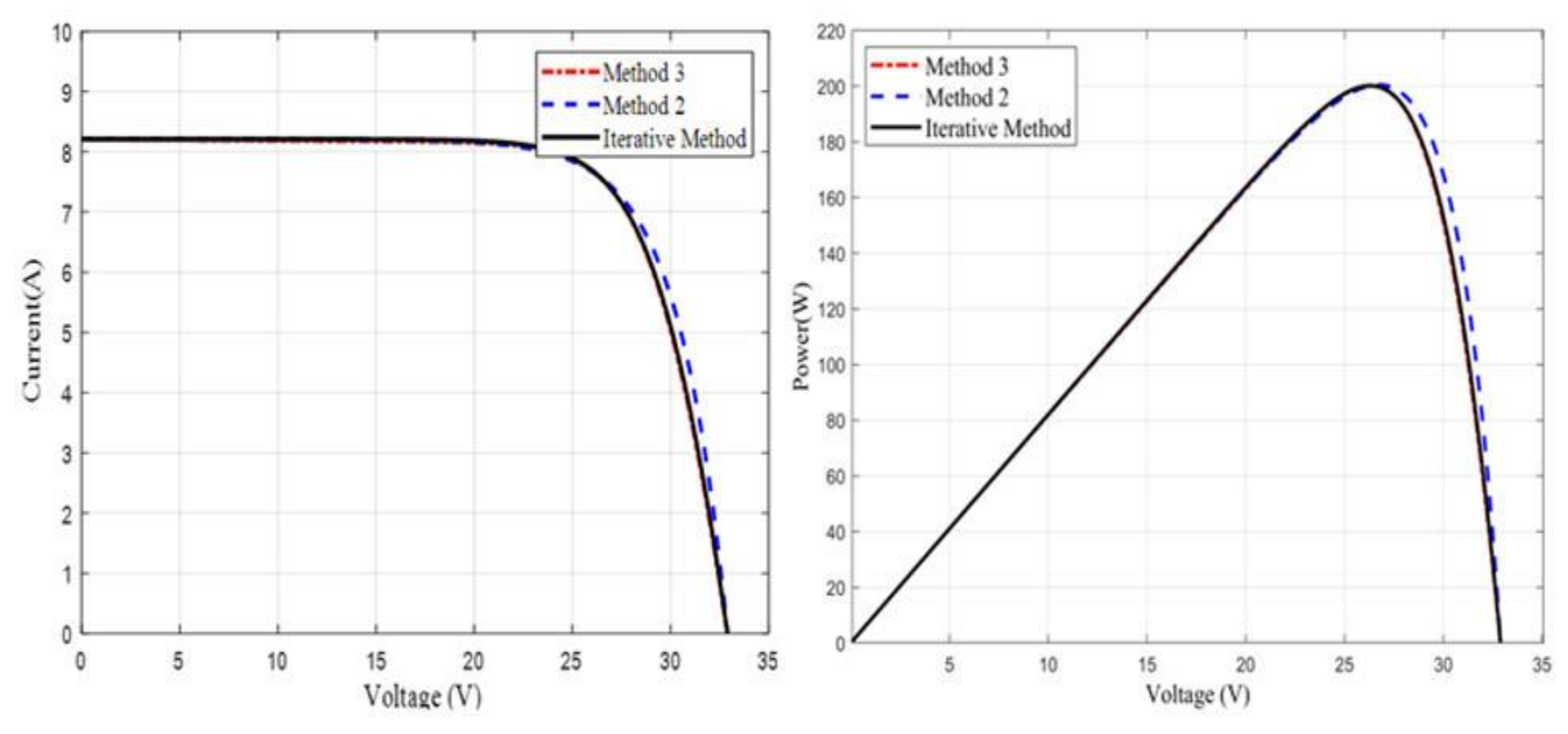
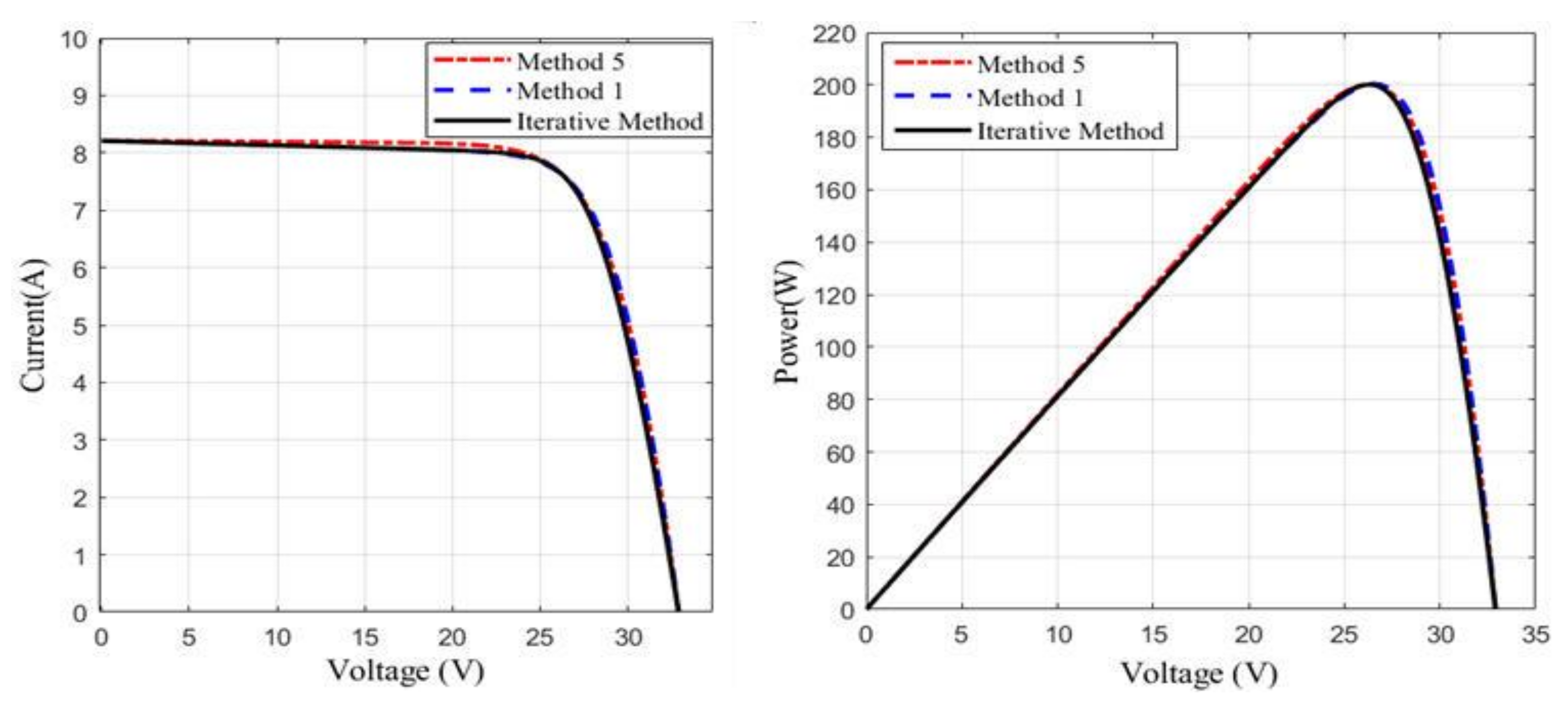
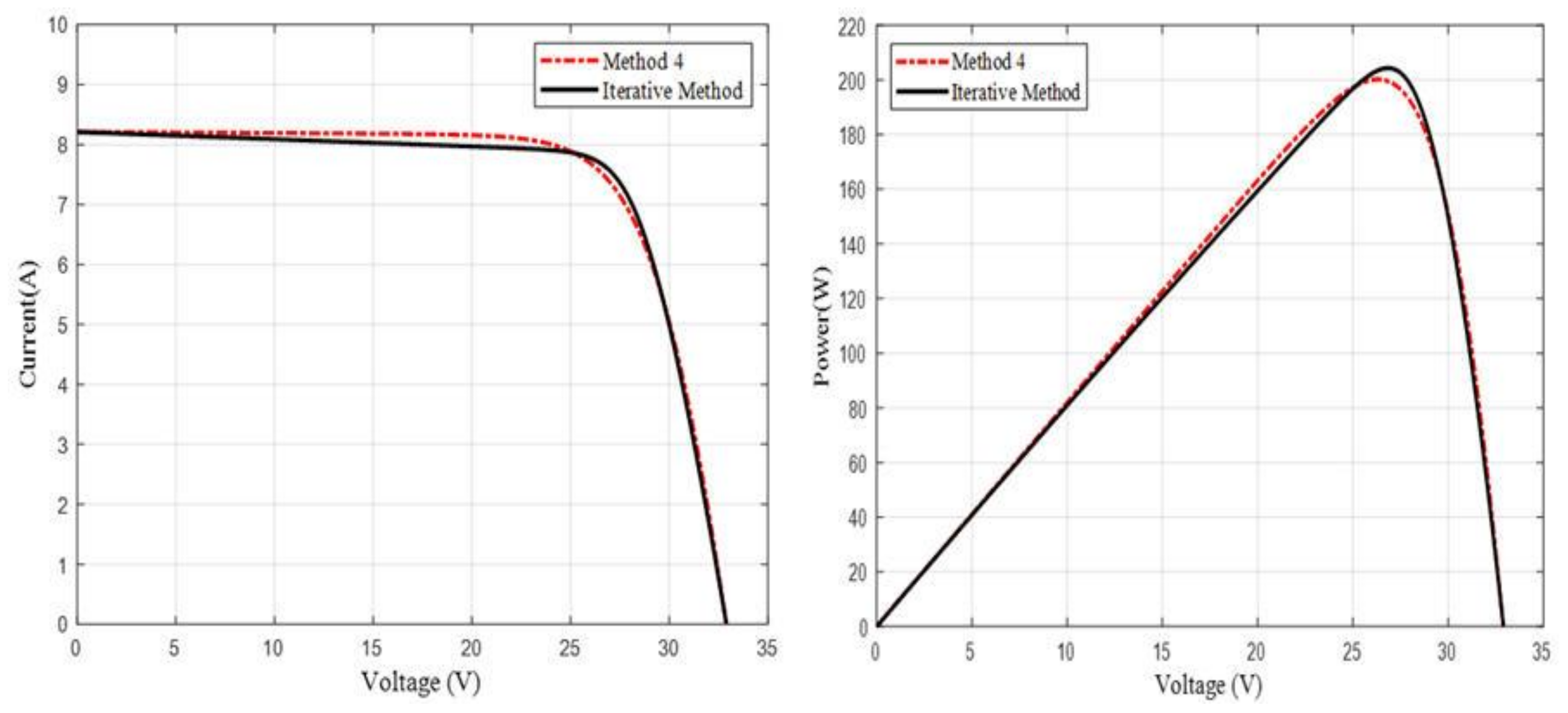
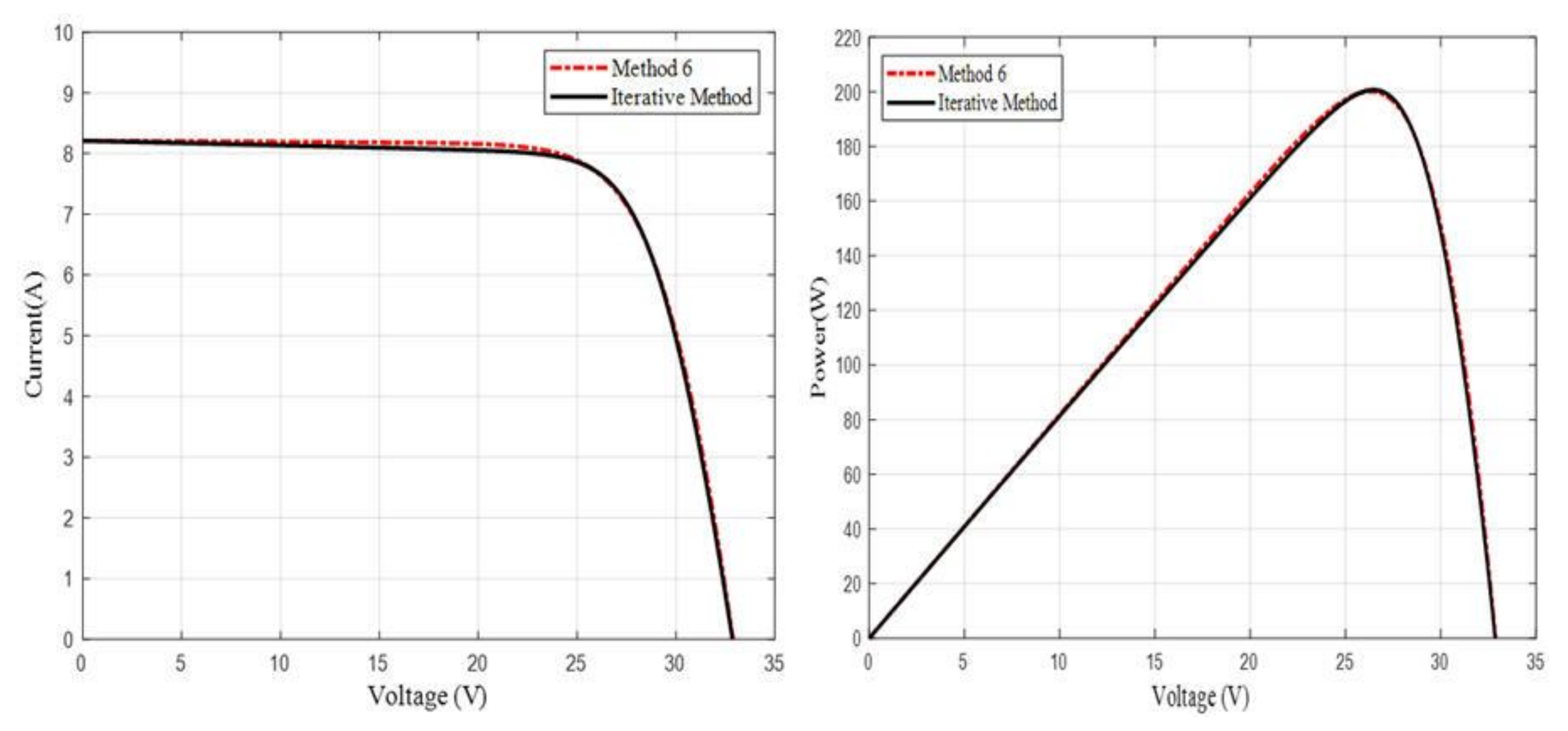
4. Results and Discussion

To synthesize the results of the analytical methods described above, software has been developed using MATLAB to extract the five parameters of the SDM model for different photovoltaic modules. Similar software has also been developed to estimate the same parameters using two numerical methods: the first uses Newton–Raphson algorithm and the initialisation provided in [34], whilst the second is based on an iterative solution procedure [14]. In order to preserve generality when comparing various methods, three photovoltaic modules of different PV technologies were used in the investigation: The multicrystalline Kyocera KC200GT [51], monocrystalline Lorentz LC50-12M [52], and thin film Sanyo 180BA19 [53]. The datasheet parameters of these test modules are summarised in Table 1. The results for the analytical and numerical methods are shown in Table 2, Table 3 and Table 4. It is evident from Table 2, that the reference results of the iterative [14] and the numerical method [34] are close as expected. For the monocrystalline and thin-film PV modules used in this investigation, the Newton–Raphson method failed to converge, see Table 3 and Table 4, demonstrating the convergence difficulties that can accompany numerical methods. From Table 2, Table 3 and Table 4, methods one and five outperform all other analytical methods and are most accurate in the case of multi and monocrystalline technologies. These two methods also offer simpler mathematical formulation. They both depend on the slope of the I–V curve with the difference that method five uses the slope at the MPP for the main equation instead of the slope at the open-circuit voltage point. Methods two and three showed degraded accuracy compared to methods one and five and can result in higher and unrealistic values for the ideality factor when used with thin-film technologies. These two methods have been formulated by neglecting some model parameters to simplify the modelling process, resulting in higher than normal values for the ideality factor. Method four suffers a noticeable inaccuracy in estimating the ideality factor and saturation current for all three PV technologies. The values of the series and shunt resistances are also unrealistic. Method six depends on a procedure that is entirely different to all other methods. It results in reduced values of the ideality factor and saturation current. The value of the ideality factor is limited to 1 ± 5 % . The reduction in the ideality factor and the saturation current have an adverse effect on the accuracy of estimating the values of the series and shunt resistances.
However, it is a matter of fact that there are different combinations of the five parameters of the SDM whose I–V curve pass through the same salient points (SC, OC, and MPP) which does not necessarily imply that all these curves represent physical meaning [54]. Therefore, to verify the performance of the analytical methods to represent the behaviour of PV modules, the characteristic curves for the KC200GT module were plotted for different combination of parameters alongside those obtained using numerical methods. For example, Methods one and five outperformed Methods two and three for the parameter extraction process, however, they exhibited similar performance to Methods one and five in presenting the characteristic curves as shown in Figure 5 and Figure 6 under STC conditions.
Methods one and five exhibit similar performance, particularly in the higher current region of the I–V curve since both are based on the slope of the I–V curve in this region as shown in Figure 6. Method four slightly underestimates the I–V curve in the high current region, since it is derived on the assumption of a flat line in this region, as shown in Figure 7.
Method 6 demonstrated good agreement with the iterative method as illustrated in Figure 8. All methods resulted in similar MPP except Method four which resulted in slightly higher peak power.

5. Conclusions

The paper presented a detailed mathematical analysis and comparative evaluation of the performance of the commonly reported analytical methods for parameters extraction of the single-diode model of a PV module. Six prevalent methods have been explored and deployed to extract the parameters of three PV modules of different PV technologies. The extracted parameters were compared with reference values extracted using numerical and iterative methods. It has been confirmed that while some methods may not be the most accurate in extracting the parameters, e.g., Methods two and three, they can still provide good agreement between their I–V curves and those obtained numerically. The reduced accuracy of Method two in the parameter extraction process could be attributed to the fact that it neglects the shunt resistance which can reduce the accuracy particularly at low levels of insolation. Methods one and five use the slope of the I–V curve about the short-circuit point which led to both methods having similar results. Method four resulted in slight overestimation in the high current region of the I–V curve since it approximated the I–V curve by a straight line in this region to simplify the model equations. Method six resulted in good agreement with the iterative I–V curve. It is recommended that additional extensive investigation should study the dependence of the analytical methods on the technology and different materials of PV modules.

Author Contributions

Conceptualization, N.A.; Data curation, H.I.; Formal analysis, N.A. and H.I.; Investigation, H.I.; Methodology, N.A. and H.I.; Software, N.A. and H.I.; Supervision, N.A.; Writing—original draft, N.A. All authors have read and agreed to the published version of the manuscript.

Funding

This research received no external funding.

Conflicts of Interest

The authors declare no conflict of interest.

Nomenclature

a Modified ideality factor ( a = n N s V t h )
α I s c Temperature coefficient of the short-circuit current ( A / ° C )
β V o c Temperature coefficient of the open-circuit voltage ( V / ° C )
δ Coefficient for the single-diode model defined as a / V o c .
G Insolation (W/m2)
G S T C Insolation at standard test conditions ( W / m 2 )
ITerminal current of a photovoltaic cell or module (A)
I m p Current at the maximum power point (A)
I s c Short-circuit current (A)
I s a t Reverse saturation current (A)
I p h Photocurrent (A)
I p h , S T C Photocurrent at standard test conditions (A)
kBoltzmann’s constant ( 1.38065 × 10 23   J / K )
MPPMaximum power point
nideality factor of a PV cell/diode
N s Number of series-connected cells in a PV module
PPower (W)
P m p Power at maximum power point (W)
PVPhotovoltaic
qElectronic charge 1.602 × 10⁻¹⁹ (C)
R s Series resistance of a photovoltaic module ( Ω )
R s o The negative of the reciprocal of the slope of the I–V curve at the open-circuit voltage point
R s h Shunt resistance of a PV module ( Ω )
R s h o The negative of the reciprocal of the slope of the I–V curve at the short-circuit current point
SDMSingle-diode model
STCStandard test conditions (Insolation = 1000 W / m 2 , air mass AM = 1.5, T = 25 ° C )
TTemperature (k)
T S T C Temperature at standard test conditions ( ° C )
VTerminal voltage of a PV module (V)
V t h Thermal voltage (V)
V o c Open-circuit voltage of a PV module (V)
V m p Voltage at maximum power point (V)
V o c , S T C Open-circuit voltage of a PV module at STC (V)
W Lambert-W function

References

  1. Masters, G.M. Renewable and Efficient Electric Power Systems; Wiley: Hoboken, NJ, USA, 2004. [Google Scholar]
  2. Femia, N.; Petrone, G.; Spagnuolo, G.; Vitelli, M. Power Electronics and Control Techniques for Maximum Energy Harvesting in Photovoltaic Systems; Informa UK Limited: Colchester, UK, 2017. [Google Scholar]
  3. Cotfas, D.T.; Cotfas, P.A.; Machidon, O. Study of Temperature Coefficients for Parameters of Photovoltaic Cells. Int. J. Photoenergy 2018, 2018, 1–12. [Google Scholar] [CrossRef] [Green Version]
  4. Anani, N.; Ibrahim, H. Adjusting the Single-Diode Model Parameters of a Photovoltaic Module with Irradiance and Temperature. Energies 2020, 13, 3226. [Google Scholar] [CrossRef]
  5. Dhimish, M. Assessing MPPT Techniques on Hot-Spotted and Partially Shaded Photovoltaic Modules: Comprehensive Review Based on Experimental Data. IEEE Trans. Electron Devices 2019, 66, 1132–1144. [Google Scholar] [CrossRef] [Green Version]
  6. Esram, T.; Chapman, P.L. Comparison of Photovoltaic Array Maximum Power Point Tracking Techniques. IEEE Trans. Energy Convers. 2007, 22, 439–449. [Google Scholar] [CrossRef] [Green Version]
  7. Ma, J.; Pan, X.; Man, K.; Li, X.; Wen, H.; Ting, T. Detection and Assessment of Partial Shading Scenarios on Photovoltaic Strings. IEEE Trans. Ind. Appl. 2018, 54, 6279–6289. [Google Scholar] [CrossRef]
  8. Bi, Z.; Ma, J.; Wang, K.; Man, K.L.; Smith, J.S.; Yue, Y. Identification of Partial Shading Conditions for Photovoltaic Strings. IEEE Access 2020, 8, 75491–75502. [Google Scholar] [CrossRef]
  9. Mäki, A.; Valkealahti, S. Power Losses in Long String and Parallel-Connected Short Strings of Series-Connected Silicon-Based Photovoltaic Modules Due to Partial Shading Conditions. IEEE Trans. Energy Convers. 2012, 27, 173–183. [Google Scholar] [CrossRef]
  10. Ibrahim, H.; Anani, N. Variation of the performance of a PV panel with the number of bypass diodes and partial shading patterns. In Proceedings of the 2019 International Conference on Power Generation Systems and Renewable Energy Technologies (PGSRET), Istanbul, Turkey, 26–27 August 2019; Institute of Electrical and Electronics Engineers (IEEE): Piscataway Township, NJ, USA, 2019; pp. 1–4. [Google Scholar]
  11. Ibrahim, H.; Anani, N. Performance of Different PV Array Configurations under Different Partial Shading Conditions. In Advances in Wireless Communications and Applications; Springer Science and Business Media LLC: Berlin/Heidelberg, Germany, 2019; pp. 445–454. [Google Scholar]
  12. Ibrahim, H.; Anani, N. Study of the Effect of Different Configurations of Bypass Diodes on the Performance of a PV String. In Advances in Wireless Communications and Applications; Springer Science and Business Media LLC: Berlin/Heidelberg, Germany, 2019; pp. 593–600. [Google Scholar]
  13. Xiao, W.; Dunford, W.G.; Capel, A. A novel modeling method for photovoltaic cells. In Proceedings of the 2004 IEEE 35th Annual Power Electronics Specialists Conference (IEEE Cat. No.04CH37551), Aachen, Germany, 20–25 June 2004; Institute of Electrical and Electronics Engineers (IEEE): Piscataway Township, NJ, USA, 2004. [Google Scholar]
  14. Villalva, M.; Gazoli, J.R.; Filho, E. Comprehensive Approach to Modeling and Simulation of Photovoltaic Arrays. IEEE Trans. Power Electron. 2009, 24, 1198–1208. [Google Scholar] [CrossRef]
  15. Siddique, H.A.B.; Xu, P.; De Doncker, R.W. Parameter extraction algorithm for one-diode model of PV panels based on datasheet values. In Proceedings of the 2013 International Conference on Clean Electrical Power (ICCEP), Alghero, Italy, 11–13 June 2013; Institute of Electrical and Electronics Engineers (IEEE): Piscataway Township, NJ, USA, 2013; pp. 7–13. [Google Scholar]
  16. Tian, H.; Mancilla-David, F.; Ellis, K.; Muljadi, E.; Jenkins, P. A cell-to-module-to-array detailed model for photovoltaic panels. Sol. Energy 2012, 86, 2695–2706. [Google Scholar] [CrossRef]
  17. Ibrahim, H.; Anani, N. Variations of PV module parameters with irradiance and temperature. Energy Procedia 2017, 134, 276–285. [Google Scholar] [CrossRef]
  18. Cotfas, D.T.; Cotfas, P.; Kaplanis, S. Methods to determine the dc parameters of solar cells: A critical review. Renew. Sustain. Energy Rev. 2013, 28, 588–596. [Google Scholar] [CrossRef]
  19. De Soto, W.; Klein, S.; Beckman, W. Improvement and validation of a model for photovoltaic array performance. Sol. Energy 2006, 80, 78–88. [Google Scholar] [CrossRef]
  20. Phang, J.; Chan, D.; Phillips, J. Accurate analytical method for the extraction of solar cell model parameters. Electron. Lett. 1984, 20, 406. [Google Scholar] [CrossRef]
  21. Aldwane, B. Modeling, simulation and parameters estimation for Photovoltaic module. In Proceedings of the 2014 First International Conference on Green Energy ICGE 2014, Sfax, Tunisia, 25–27 March 2014; Institute of Electrical and Electronics Engineers (IEEE): Piscataway Township, NJ, USA, 2014; pp. 101–106. [Google Scholar]
  22. Saloux, E.; Teyssedou, A.; Sorin, M. Explicit model of photovoltaic panels to determine voltages and currents at the maximum power point. Sol. Energy 2011, 85, 713–722. [Google Scholar] [CrossRef]
  23. Louzazni, M.; Khouya, A.; Crăciunescu, A.; Amechnoue, K.; Mussetta, M. Modelling and Parameters Extraction of Flexible Amorphous Silicon Solar Cell a-Si:H. Appl. Sol. Energy 2020, 56, 1–12. [Google Scholar] [CrossRef]
  24. Luo, X.; Cao, L.; Wang, L.; Zhao, Z.; Huang, C. Parameter identification of the photovoltaic cell model with a hybrid Jaya-NM algorithm. Optik 2018, 171, 200–203. [Google Scholar] [CrossRef]
  25. AlRashidi, M.; Alhajri, M.; El-Naggar, K.; Al-Othman, A. A new estimation approach for determining the I–V characteristics of solar cells. Sol. Energy 2011, 85, 1543–1550. [Google Scholar] [CrossRef]
  26. Gude, S.; Jana, K.C. Parameter extraction of photovoltaic cell using an improved cuckoo search optimization. Sol. Energy 2020, 204, 280–293. [Google Scholar] [CrossRef]
  27. Gong, W.; Cai, Z. Parameter extraction of solar cell models using repaired adaptive differential evolution. Sol. Energy 2013, 94, 209–220. [Google Scholar] [CrossRef]
  28. Chan, D.; Phang, J. Analytical methods for the extraction of solar-cell single- and double-diode model parameters from I-V characteristics. IEEE Trans. Electron Devices 1987, 34, 286–293. [Google Scholar] [CrossRef]
  29. Hejri, M.; Mokhtari, H.; Azizian, M.R.; Ghandhari, M.; Söder, L. On the Parameter Extraction of a Five-Parameter Double-Diode Model of Photovoltaic Cells and Modules. IEEE J. Photovolt. 2014, 4, 915–923. [Google Scholar] [CrossRef]
  30. Sera, D.; Teodorescu, R.; Rodriguez, P. Photovoltaic module diagnostics by series resistance monitoring and temperature and rated power estimation. In Proceedings of the 2008 34th Annual Conference of IEEE Industrial Electronics, Orlando, FL, USA, 10–13 November 2008; Institute of Electrical and Electronics Engineers (IEEE): Piscataway Township, NJ, USA, 2008; pp. 2195–2199. [Google Scholar]
  31. Haouari-Merbah, M.; Belhamel, M.; Tobias, I.; Ruiz, J. Extraction and analysis of solar cell parameters from the illuminated current–voltage curve. Sol. Energy Mater. Sol. Cells 2005, 87, 225–233. [Google Scholar] [CrossRef]
  32. Lim, L.H.I.; Ye, Z.; Ye, J.; Yang, D.; Du, H. A Linear Identification of Diode Models from Single II– VVCharacteristics of PV Panels. IEEE Trans. Ind. Electron. 2015, 62, 4181–4193. [Google Scholar] [CrossRef] [Green Version]
  33. Ortiz-Rivera, E.I.; Peng, F. Analytical Model for a Photovoltaic Module using the Electrical Characteristics provided by the Manufacturer Data Sheet. In Proceedings of the IEEE 36th Conference on Power Electronics Specialists, Recife, Brazil, 16 June 2005; Institute of Electrical and Electronics Engineers (IEEE): Piscataway Township, NJ, USA, 2006; pp. 2087–2091. [Google Scholar]
  34. Can, H.; Ickilli, D. Parameter Estimation in Modeling of Photovoltaic Panels Based on Datasheet Values. J. Sol. Energy Eng. 2013, 136, 021002. [Google Scholar] [CrossRef]
  35. Mahmoud, Y.; Xiao, W.; Zeineldin, H.H. A Parameterization Approach for Enhancing PV Model Accuracy. IEEE Trans. Ind. Electron. 2012, 60, 5708–5716. [Google Scholar] [CrossRef]
  36. Chatterjee, A.; Keyhani, A.; Kapoor, D. Identification of Photovoltaic Source Models. IEEE Trans. Energy Convers. 2011, 26, 883–889. [Google Scholar] [CrossRef]
  37. Batzelis, E.; Routsolias, I.A.; Papathanassiou, S.A. An Explicit PV String Model Based on the Lambert WW. Function and Simplified MPP Expressions for Operation Under Partial Shading. IEEE Trans. Sustain. Energy 2013, 5, 301–312. [Google Scholar] [CrossRef]
  38. De Blas, M.; Torres, J.; Prieto, E.; García, A. Selecting a suitable model for characterizing photovoltaic devices. Renew. Energy 2002, 25, 371–380. [Google Scholar] [CrossRef]
  39. Kennerud, K. Analysis of Performance Degradation in CdS Solar Cells. IEEE Trans. Aerosp. Electron. Syst. 1969, 5, 912–917. [Google Scholar] [CrossRef]
  40. Cubas, J.; Pindado, S.; Victoria, M. On the analytical approach for modeling photovoltaic systems behavior. J. Power Sources 2014, 247, 467–474. [Google Scholar] [CrossRef] [Green Version]
  41. Mahmoud, Y.; Xiao, W.; Zeineldin, H.H. A Simple Approach to Modeling and Simulation of Photovoltaic Modules. IEEE Trans. Sustain. Energy 2012, 3, 185–186. [Google Scholar] [CrossRef]
  42. Mahmoud, Y.; El-Saadany, E.F. Accuracy Improvement of the Ideal PV Model. IEEE Trans. Sustain. Energy 2015, 6, 1–3. [Google Scholar] [CrossRef]
  43. Wanger, A. Peak power and internal series resistance measurements under natural ambient conditions. In Proceedings of the EuroSun Conference, Dortmund, Denmark, 19–22 June 2000. [Google Scholar]
  44. Ishaque, K.; Salam, Z.; Taheri, H. Simple, fast and accurate two-diode model for photovoltaic modules. Sol. Energy Mater. Sol. Cells 2011, 95, 586–594. [Google Scholar] [CrossRef]
  45. Bai, J.; Liu, S.; Hao, Y.; Zhang, Z.; Jiang, M.; Zhang, Y. Development of a new compound method to extract the five parameters of PV modules. Energy Convers. Manag. 2014, 79, 294–303. [Google Scholar] [CrossRef]
  46. Orioli, A.; Di Gangi, A. A procedure to calculate the five-parameter model of crystalline silicon photovoltaic modules on the basis of the tabular performance data. Appl. Energy 2013, 102, 1160–1177. [Google Scholar] [CrossRef]
  47. Charles, J.; Abdelkrim, M.; Muoy, Y.; Mialhe, P. A practical method of analysis of the current-voltage characteristics of solar cells. Sol. Cells 1981, 4, 169–178. [Google Scholar] [CrossRef]
  48. Brano, V.L.; Orioli, A.; Ciulla, G.; Di Gangi, A. An improved five-parameter model for photovoltaic modules. Sol. Energy Mater. Sol. Cells 2010, 94, 1358–1370. [Google Scholar] [CrossRef]
  49. Batzelis, E.; Papathanassiou, S.A. A Method for the Analytical Extraction of the Single-Diode PV Model Parameters. IEEE Trans. Sustain. Energy 2015, 7, 504–512. [Google Scholar] [CrossRef]
  50. Batzelis, E.; Kampitsis, G.E.; Papathanassiou, S.A.; Manias, S. Direct MPP Calculation in Terms of the Single-Diode PV Model Parameters. IEEE Trans. Energy Convers. 2014, 30, 226–236. [Google Scholar] [CrossRef]
  51. Kyocera North America, “KC200GT solar module,” Kyocera Solar. Available online: https://www.kyocerasolar.com/dealers/product-center/archives/spec-sheets/KC200GT.pdf (accessed on 20 December 2019).
  52. Lorentz Solar Modules, “LC50-12M”. Available online: www.deparsolar.com/images/dosya/LC50_12M.pdf (accessed on 10 March 2020).
  53. Sanyo, “Sanyo 180BA19”. Available online: www.ecodirect.com/Sanyo-HIP-180BA19-180-Watt-p/sanyo-hip-180ba19.htm (accessed on 20 June 2019).
  54. Carrero, C.; Rodriguez, J.; Ramirez, D.; Platero, C. Simple estimation of PV modules loss resistances for low error modelling. Renew. Energy 2010, 35, 1103–1108. [Google Scholar] [CrossRef]
Figure 1. Normalised experimental current–voltage (I–V) and power–voltage (P–V) characteristics of a generic PV generator.
Energies 13 04825 g001
Figure 2. The single-diode model of a photovoltaic (PV) generator.
Energies 13 04825 g002
Figure 3. The idealised single-diode model (SDM) model of a PV generator.
Energies 13 04825 g003
Figure 4. The four-parameters SDM.
Energies 13 04825 g004
Figure 5. Comparison between the I–V (left) and P–V (right) curves obtained using Methods two and three with those obtained using numerical method for the KC200GT module.
Energies 13 04825 g005
Figure 6. Comparison between the I–V (left) and P–V (right) curves obtained using Methods one and five with those obtained using numerical method for the KC200GT module.
Energies 13 04825 g006
Figure 7. Comparison between the I–V (left) and P–V (right) curves obtained using Method four with those obtained using numerical method for the KC200GT module.
Energies 13 04825 g007
Figure 8. Comparison between the I–V (left) and P–V (right) curves obtained using Method six with those obtained using numerical method for the KC200GT module.
Energies 13 04825 g008
Table 1. Parameters for the Multi-crystalline (Kyocera KC200GT).
DatasheetKC200GTLC50-12M180BA19
ParametersMulti-CrystallineMono-CrystallineThin Film
I s c A 8.21 A3.2 A3.65 A
V o c V 32.9 V22.5 V66.4 V
I m p A 7.61 A2.9 A3.33 A
V m p V 26.3 V17.2 V54 V
µ V o c ( V / ° C ) −1.23 × 10⁻¹ −7.88 × 10⁻² −173 × 10−3
µ I s c ( A / ° C ) 3.18 × 10⁻³ 2.88 × 10⁻³ 1.01 × 10⁻³
N s 543696
Table 2. Parameters for the Multicrystalline (Kyocera KC200GT).
MethodParameter
n R s R s h I s a t I p h
Method 11.083170.270771242.4885 × 10−98.22793
Method 21.817640infinite1.78074 × 10−58.21
Method 31.409910.19455infinite4.09919 × 10−78.21
Method 40.650080.3999982.55081.14541 × 10−158.24978
Method 50.884230.38033123.621.81544 × 10−118.23526
Method 61.002580.30567130.4664.43777 × 10−108.22924
Iterative [14]1.30.2283572.1249.89443 × 10−88.21329
Numerical [34]1.34050.2172951.3271.7097 × 10−78.2119
Table 3. Parameters for the Monocrystalline (Lorentz LC50-12M).
MethodParameter
n R s R s h I s a t I p h
Method 12.03610.100452062.0109 × 10−53.20156
Method 22.4197901.3832 × 10−43.2
Method 31.761870.49693.24464 × 10−63.2
Method 40.793420.93255105.704141.47618 × 10−133.22823
Method 51.242540.77359205.226419.82922 × 10−93.21206
Method 60.996930.84024125.536998.22168 × 10−113.22142
Iterative method [14]1.20.784186.405745.06574 × 10−93.21352
Numerical method [19]No convergence
Table 4. Parameters for the Thin film (Sanyo 180BA19).
MethodParameter
n R s R s h I s a t I p h
Method 10.557672.6900423293.99938 × 10−213.65422
Method 22.0645507.9701 × 10−63.65
Method 32.11483−0.090681.08651 × 10−53.65
Method 40.957291.13544313.851292.13594 × 10−123.6632
Method 51.951450.106572328.89343.71538 × 10−63.65017
Method 60.955891.41883327.955252.1766 × 10−123.66579
Iterative [14]1.80.273001181.565091.17348 × 10−123.65084
Numerical method [19]No convergence

