Abstract
The transient liquid crystal thermography can be a suitable tool to study heat-transfer performances on internal cooling schemes of gas turbine blades. One of the hot topics related to this methodology is about the level of reliability of the heat-transfer assessments in rotating tests where the fluid experiences time-dependent rotating effects. The present study contribution aims to experimentally validate by cross-comparison of the outcomes obtained by employing the transient technique with those from the steady-state liquid crystal thermography in which the rotational effects occur as time-stable by definition. Heat-transfer measurements have been conducted on a rib-roughened square cross-section channel, with an inlet Reynolds number equal to 20,000 and rotation number up to 0.2. Special attention has been paid to the definition of the more reliable calibration strategy for liquid crystals that are employed in the transient thermography and to the proper estimation of the heat losses in the post-processing of the steady-state experimental data. The results show great accordance between the indications provided by the two techniques both in static and rotating conditions, demonstrating the possibility to exploit the advantages of the transient liquid crystal thermography for the investigation of heat transfer into rotating cooling channels.
1. Introduction
The liquid crystal thermography (LCT) provides a suitable and accurate experimental technique to evaluate wall temperatures. Its convenience is due to the reversible and repeatable behaviour of the thermochromic liquid crystals: they show a selective light reflection in the visible spectrum as a function of the temperature of the surface onto which they are painted. The temperature information delivered by the LCT technique has been extensively used to accomplish spatially resolved heat-transfer measurements for internal and external flow applications [1], either in steady-state or transient experiments. Among the possible applications of LCT, the investigation about the thermal behaviour of gas turbine internal cooling passages has made wide use of this methodology for many years, starting from the first examples of LCT using the steady-state approach on simple geometries [2] to the application of the transient LCT technique in more complex ones [3], to cite few examples among many others. When passages for turbine rotor blades are considered, different constraints arise, as it will be discussed later on, imposing to conduct the experiment with more attention and under particular boundary conditions. At present, some issues about the application of transient LCT in a rotating cooling channel are still open, and this contribution aims to shed some light on these aspects.
In a transient experiment, starting from an isothermal condition between the airflow and the wetted channel surfaces, a sudden change in the flow temperature is imposed to trigger the heat-transfer process. Then, the computation of the heat-transfer coefficient (HTC) relies on the one-dimensional Fourier’s equation written for a semi-infinite solid using the surface and flow-temperature evolutions as boundary conditions [4]. Schultz et al. [5] evaluated the maximum duration of a transient test within which a flat wall can be properly assumed as a semi-infinite solid. However, those assumptions are not applicable for every experiment, such as when thin and highly curved walls are considered (e.g., leading-edge areas of a turbine blade). In this case, simple curvature correction can be adopted [6] or exact heat conduction models have to be implemented to deal with the curvature and finite thickness of walls [7]. The 1D conduction assumption is taken to be valid as long as the surface does not present large traverse temperature variations. Several papers [8,9] address the lateral conduction error that is involved when significant surface temperature gradients arise and propose alternative HTC evaluation procedures to correct the analytical 1D solution without solving the 3D energy equation. These aspects continue to have the proper attention from the research community as demonstrated by the recent contributions from Ahmed et al. [10] where a new method to solve the 3D conduction equation is proposed for a more accurate determination of the heat-transfer coefficient in the occurrence of strong lateral conduction.
In addition to the mathematical aspects above-mentioned, attention has to be paid on test conditions under which the experiments are conducted. In real gas turbine blade cooling systems, the air is taken from the last compressor stages of the engine and, then, is routed through complex passages inside the turbine blade to provide adequate cooling of the material; consequently, the airflow is colder than the surfaces of the passages housed inside the blade. Conversely, in transient LCT experiments, the investigated channel wall is commonly exposed to a hot mainstream generated by electric mesh heaters [11,12,13]. This way to proceed is very popular, because it is rather simple to implement and is acceptable as long as the stationary cooling passages are concerned (i.e., cooling schemes of stator turbine blades). When rotation takes place, it induces the development of Coriolis and centrifugal buoyancy forces that are dependent on the thermal conditions of fluid and channel walls. Therefore, a sudden temperature drop on the flow instead of a flow heating should be imposed to satisfy the similarity with real working conditions. Pagnacco et al. [14] applied the transient LCT technique to study the heat-transfer distribution in a rotating square ribbed channel at a Reynold number equal to 10,000 and rotation number up to 0.4. The authors highlighted the different heat-transfer behaviour and opposite buoyancy effects depending on the direction of the flow-temperature change realized on the airflow (i.e., cold or hot variations). The reported outcomes confirm the need to move for the cold step methodology with the aim to achieve meaningful heat-transfer data about the turbine blades cooling problems. For this reason, the current contribution implements the transient LCT in which the airflow is cooled under the room temperature, although this has led to more complexity in the air treatment system of the experimental facility. In the open literature, few contributions make use of the transient LCT approach implementing a fluid cold temperature step to investigate about rotating cooling channels. Among these, the most significant and numerous contributions come from Ekkad et al. Starting from the first work reported in 2012, a number of different channel configurations have been investigated with the attention on the effects of ribs geometry [15], channel orientation [16,17], and multi-pass configuration with optimized layouts to minimize the Coriolis effect [18,19]. A rig capable to reach extremely high rotational speeds has been designed and commissioned at the University of Stuttgart in Germany [20], but at the moment, only preliminary data have been published.
In the data processing of the transient LCT technique, HTC is implicitly assumed to be constant throughout the entire experiment [4]. However, the Coriolis effect and the buoyancy forces are actually changing during a transient rotating test because of the wall and flow-temperature variations required by the transient approach. This aspect is not taken into consideration in the literature, also because in many cases, the test conditions are such to make buoyancy forces negligible [16,17].
One of the aims of the present contribution is to investigate the effect of buoyancy force evolution during a transient LCT experiment on the resulting heat-transfer coefficient. A possible way to do this, here exploited, is the comparison of the transient results with those experimentally obtained by means of a steady-state approach (e.g., steady-state LCT), where flow and model temperature are time-stable by definition (and so are rotation-induced effects). Even if a very common and simplified cooling channel geometry has been chosen as a case study, the data available in the open literature for validation purposes are pretty much scattered [21,22,23], as it will be clarified in the results discussion. The complexity in replicating the intake conditions together with the low consistency of the literature data have, hence, led to perform also the steady-state LCT on the investigated channel in order to collect more reliable heat-transfer information to be used as references for the validation of the transient experiments.
Transient LCT with cold temperature change is more easily performed making use of liquid crystals (LC) with activation temperatures below a standard laboratory environmental temperature. This means that the LC stay for most of their life in the melted phase (i.e., above their clearing point) and are employed throughout cooling in transient tests. Several contributions in the literature [24,25,26] suggest a different colour response on cooling and heating (i.e., hysteresis phenomenon) for the LC with activation temperature above the environmental temperature. However, no thorough contributions seem to be available about the behaviour of LC that exhibits the colour play below room temperature. Given this lack of information, in this paper, an investigation about the calibration procedure and exploitation strategy has been also performed to get reliable temperature indications out of them.
2. Experimental Setups and Methodologies
2.1. Channel Geometry and Test Conditions
The heat-transfer measurements by means of the two LCT approaches have been performed on a simplification of an internal cooling passage of a turbine blade. The channel geometry and its spatial orientation are depicted in Figure 1. The channel model has a scale factor of about 20 allowing us to perform spatially detailed HTC distributions. The resulting channel length is 1000 mm with a constant square cross-section of 50 50 mm that corresponds to a hydraulic diameter equal to 50 mm. On one side, 16 squared ribs are installed with the angle of attack of 90 degrees with respect to the main channel axis (i.e., the principal flow direction), the blockage ratio is 0.1, and the rib pitch-to-height ratio is 10. The first 200 mm at the channel inlet are kept smooth. The reference frame relative to the channel has the x-axis perpendicular to the ribbed wall, the y-axis towards the radial direction, and the z-axis parallel to the ribs. The model spins around the Z-axis of the global reference frame with angular velocity .
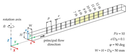
Figure 1.
Sketch of geometry and coordinate system of the test section.
The experimental campaign has focused on the HTC distribution on the ribbed surface between the 7th and the 13th rib ( 10 16 from the test section inlet). The representative inlet test conditions are kept constant at a Reynolds number (Equation (1)) of 20,000 and rotation number (Equation (2)) equal to 0, 0.1, and 0.2. The direction of rotation has been set in order to have the ribbed wall that acts as the trailing side.
Since steady-state and transient LCT approaches require different setups of the test article, two different channel models have been built. The details about models manufacturing and instrumentation are provided in the following subsections in which the two measurement approaches are also described.
2.2. Rotating Channel Facility
The test facility of the Energy and Environmental Engineering Laboratory of the University of Udine (see Figure 2) allows performing heat-transfer measurements on rotating channels. At the present progress of the test rig, both LCT approaches can be conducted. Its development, main features, and an example of application are thoroughly described in a previous contribution [27], and for this reason, only the main features are described in the following. Models under test are fixed on one side of the rotating arm of 3 m diameter that spins around the vertical axis. The rotating arm is constrained to the metallic supporting frame by the slewing bearing, and its rotation is driven by a 11 kW electric motor through the transmission belt. The process air enters along the rotation axis in the settling chamber, which is designed in such a way to feed the channel with a uniform velocity distribution at the inlet. Then, the fluid flows radially outward through the test section at which end it is collected by the returning pipeline towards the hollow shaft of the electro-fluidic junction. The air is sucked out by a centrifugal fan, and the mass flow rate is continuously measured by means of a calibrated orifice flow meter [28] located upstream of the fan.
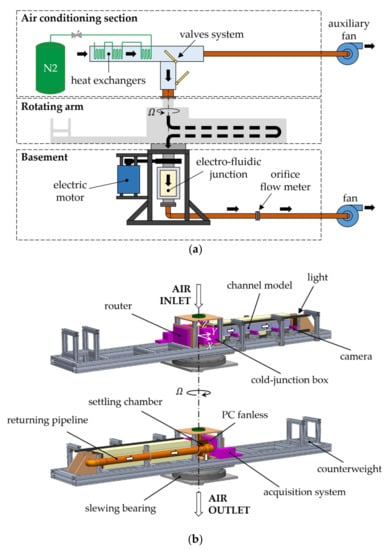
Figure 2.
Test facility: (a) schematic view; (b) virtual model of the equipped rotating arm.
During transient LCT, the airflow has to undergo a sudden cooling to satisfy similarity with the real working conditions. This task is accomplished by using the air cooling section located upstream of the settling chamber inlet. The cooling system is composed of fin-tube heat exchanger that is fed by liquid nitrogen and a valve set that can switch the system in two operation modes: the pre-test phase and test phase. In the pre-test phase, room air is routed into the channel model to maintain an isothermal condition with the channel walls. Meanwhile, an auxiliary fan sucks a secondary airflow through the heat exchanger to reach the target condition for the experiment, monitoring the flow temperature at the heat exchanger outlet. The mass flow rates that run in the two circuits are regulated in order to have the same Reynolds number referred to the hydraulic diameter of the channel model. The test phase starts when the suitable condition of the secondary flow is reached. The valves are switched, the auxiliary fan is turned off, and the cooled air is routed into the channel. During the test phase, mass flow rate and angular velocity of the rotating arm are continuously adjusted to maintain constant both Reynolds and rotation numbers, despite the large variation of the flow temperature [27]. For the tests with the steady-state LCT approach, the air cooling section is not employed and air at ambient temperature flows inside the channel. An on-ground DC power supply is connected through the electro fluidic junction to the channel-wall heater, details of which are given in the next subsection.
The acquisition system is equipped on board the rotating arm, and it has the tasks to capture the colour play of the LC, to acquire the airflow temperature, and to send all the collected data to an on-ground computer. Two frame grabber cameras (BASLER acA1300-60gc camera with the NAVITAR 6 mm 1:1.4 C ½″ M30.5 camera lens) are installed with their optical axis orthogonal to the ribbed surface and the image are acquired from the fluid side. Two LED strips (120 led/m, 24 W/m, and 4000 K of colour temperature) evenly illuminate the ribbed wall reducing issues related to radiative effects on the measurement surface. Flow-temperature variation is measured using thermocouples, which are immersed in the bulk flow at different positions that are provided in the next subsections. The scanning of the thermocouples signals is performed by the National Instrument (NI) cRIO-9074 device equipped with NI 9213 module. All the cold junctions of the thermocouples are realized inside an aluminium slab; the temperature of which is monitored by a resistance temperature detectors (PT100). This temperature is used as the reference junction temperature to apply for cold junction compensation. An on-board fanless computer deals with the managing of the acquisition systems and with the collecting and transferring of the entire acquired data to an on-ground computer via networking devices. During the transient tests, the cameras record sequences of frames that are synchronized with the temperature acquisitions by means of a 25 Hz trigger signal generated by the NI myDAQ unit. For the steady-state LCT approach, the temperature of the ribbed surface is kept in the active range of the LC by controlling the supplied electric power. Steady thermal condition is considered to be reached when the surface temperature is stable over a time interval of at least 15 min, after which the cameras take images of the investigated surface.
2.3. Steady-State Liquid Crystals Thermography
Figure 3 provides a schematic representation of the test article employed in the steady-state LCT experiments. The channel is formed by plexyglass (PMMA) walls of 12 mm thickness. A 25 μm thick Inconel 665 alloy foil provides the required heat flux by Joule effect onto the entire ribbed area. The foil has a width of 48 mm and is attached by means of an adhesive layer, then the ribs (as well made of PMMA) are glued on the Inconel surface. Copper bars strongly soldered at both ends of the foil allow providing a uniform power supply to it. The channel is externally covered by a 50 mm layer of polyurethane foam to reduce the conductive heat losses. Two K-type thermocouples monitor the outer surface temperature of the insulating coat to provide the information that is necessary for heat losses estimation. The inlet and outlet temperature conditions of the flow are taken by two K-type thermocouples, which are installed in the centre of the respective channel section. Matt black paint SPB100 Hallcrest is sprayed on the ribbed and sidewalls to avoid annoying reflections and acting as a background to enhance the colours of the liquid crystals. Then, the R35C7W Hallcrest wide-banded LC are applied only on the investigated surface, according to the procedure of surface preparation exposed in [29]. The selected LC present a nominal starting temperature of 35 °C and a colour bandwidth of 7 °C.
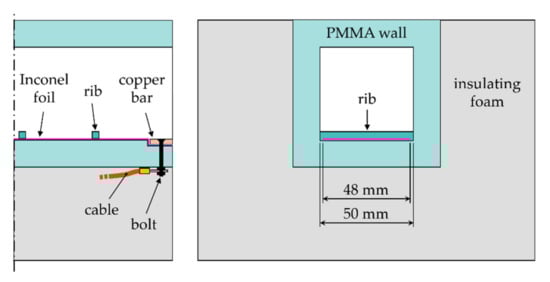
Figure 3.
Sketch of the test article used in the steady-state liquid crystal thermography (LCT) experiments.
The local HTC can be evaluated by:
The fluid temperature is computed by linear interpolation of the inlet and outlet fluid temperatures; this is a good assumption given the selected geometry and test conditions (i.e., uniform heat flux and straight channel with a constant cross-section). The wall temperature is obtained from the colour indication of the LC by applying the calibration curve that will be defined in the next subsection. The hue parameter is computed for each pixel of the image by an in-house developed routine that also maps the images into the real model geometry. The latter task is accomplished by means of a camera spatial calibration procedure, as described in [27]. The convective heat flux in Equation (3) differs from the one generated by the heater element by the heat flux losses . The heat generated by Joule effect is calculated by knowing the electrical resistance of the Inconel foil and measuring the voltage drop across the heater. The losses term can be decomposed in two contributions: the conductive heat loss through the channel walls , and the radiative heat loss between the channel inner surfaces . Their correct evaluations are of paramount importance for the accuracy of the HTC values. For this reason, two numerical models have been built in ANSYS CFX (v17.0, ANSYS Inc., Canonsburg, PA, USA) to perform thermal analyses that allow for considering the radiative and conductive phenomena. The radiative model considers only the air volume enclosed by the channel walls, since the PMMA is opaque to infrared radiation. Additionally, air is considered only as radiative medium (i.e., the flow field is not simulated), and therefore, only the discrete radiative transfer mode surface to surface is set in the ANSYS CFX configuration. The wall temperatures that come from the solution of the conductive model and emissivities of the surfaces are imposed as boundary conditions. The emissivity coefficient is set to 0.96 for the ribbed and sidewalls, as measured by Lucas et al. [30] for a layer of liquid crystals painted over a black matt paint. The emissivity of the remaining side (i.e., wall for the optical accessibility) is assumed equal to 0.86—the value taken is from the PMMA datasheet. The conductive model comprises a section of the channel from the 7th to the 13th rib that consists of channel walls, the external insulating layer, and the Inconel foil, as illustrated in Figure 4a. The computational domain has been discretized by a block-structured grid with quadrilateral cells. A single layer of elements has been judged sufficient to discretize the thickness of the heating element. The mesh dimensions of the other sub-domains are set at the interface with the side dimension of the Inconel cells width, which has been determined by means of grid independence test. Starting from a cell width of 1 mm, this dimension was progressively reduced by steps of 0.25 mm until the numerical solution did not change by less of 1%. The final cell dimension has been set to 0.5 mm with a consequent final number of elements of about 1.8 M. The cross-section view of the resulting structured mesh is provided in Figure 4b. The boundary conditions of the conductive model are the following: the Inconel foil domain generates a uniform internal heat flux (equal to the electric power supplied), the limiting cross-sections are assumed adiabatic (i.e., periodic boundary condition), and a constant temperature is imposed on the external surfaces (its value results from the average of the readings from the thermocouples installed on the external surfaces of the insulating layer). Finally, convective (the unknown) and radiative (from the radiative model) heat-transfer distributions are imposed on the inner surfaces. The two described numerical models turn out to be coupled, and furthermore, the computed internal fluxes depend on the unknown HTC distribution. Therefore, an iterative loop is necessary to update the solution until convergence, as described in Figure 5a.
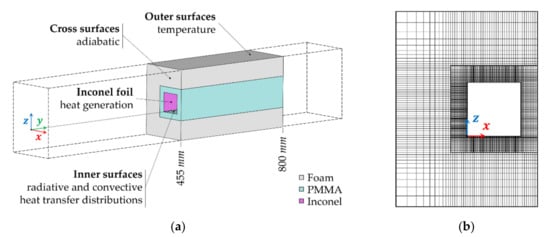
Figure 4.
Conductive numerical model: (a) domains and boundary conditions; (b) cross-section view of the computational grid.
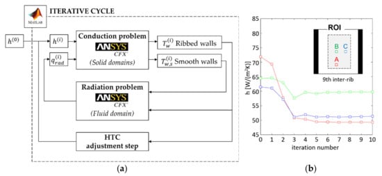
Figure 5.
Iterative procedure for steady-state data elaboration: (a) block diagram; (b) example of the heat-transfer coefficient (HTC) value convergences history for the static test.
At the first iteration, an attempt distribution of the convective heat transfer is estimated from Equation (3) by neglecting the heat losses, and it is used as a boundary condition for the conductive model. The latter computes the inner wall temperature distributions, which in turn, are the boundary conditions for the radiative model. Meanwhile, the temperature map of the ribbed surface and experimental one from the steady-state LCT are compared. The iterative loop continuously updates the HTC distribution by computing Equation (4) and runs the numerical simulations until the measured and calculated temperatures match.
Figure 5b reports the trends of the HTC values over the iterative procedure for three representative points taken within the 9th inter-rib area for the static condition; six iterations have been proved to be sufficient to ensure convergence. The starting value can only be computed where the LC are in their visible colour range, in contrast with the requirement of the conductive model that needs spatially continuous boundary conditions. Since regions where the LC are not active are limited to small portions of the ribbed surface near the edges, this gap is filled by extrapolating the trends of from nearby areas. Similarly, the conductive numerical analysis requires a convective HTC on the smooth walls of the channel and on the ribs’ surfaces. In these cases, averaged values are taken from the literature [31], and uniform distributions are imposed on these surfaces. These assumptions undoubtedly affect the final solution, and to clarify to which extent, a sensitivity analysis has been carried out. Additional simulations have been performed by increasing and decreasing by 50% the assumed literature values, and then, the final HTC distributions returned by the iterative procedure have been compared. In this way, the boundary of a region of interest (ROI) has been identified as reported in Figure 5b in which the solution variation is less than 2.5%, despite the large variations in the assumed values of the boundary conditions.
2.4. Transient Liquid Crystals Thermography
The channel model used in the transient tests is machined out of PMMA with a wall thickness of 15 mm. In order to exactly evaluate the HTC during the thermal transient tests, the thermo-physical properties of PMMA have to be accurately known. For this reason, two material samples have been sent to a laboratory specialized in materials analysis [32]. The thermal conductivity and the specific heat have been measured by means of differential scanning calorimetry, while the density has been indirectly calculated by weighing the samples and estimating the volume from their geometries. The flow driving temperature is provided by the indications of 8 K-type thermocouples immersed in the core flow. These thermocouples are inserted from the lateral walls and lay on the symmetry plane at the positions shown in Figure 6. The hot-junction diameters are 0.075 mm, which makes these thermocouples suitable to measure sudden temperature variations. The thermal and flow field behaviours are expected to be symmetrical with respect to the median plane orthogonal to the ribbed wall, given the symmetry of the channel geometry. For this reason, two types of narrow-banded LC with different starting temperatures are sprayed on the two halves of the ribbed surface after the application of the matt black paint SPB1000 Hallcrest. The surface has been treated and painted according to [29]. As shown in Figure 6, the R13C1W Hallcrest (LC13) is sprayed on the lower region and the R3C1W Hallcrest (LC3) on the upper area. In this way, the HTC are assessed in distinct time instants from the indications of the two LC at homologous locations, with the purpose to reveal possible time-depending rotational effects on heat transfer. Narrow-banded LC have been used rather than wide-banded LC in order to allow better accuracy [33]. In addition, Yan and Owen [34] provides some guidelines for the selection of the best-suited activation temperature of LC that ensures the minimization of the uncertainty. This can be reached if the dimensionless wall temperature:
is maintained within the range 0.3 0.7. In the present contribution, the selected LC satisfy this condition within the entire domain, as shown in Figure 7. Figure 7 reports the dimensionless wall temperature averaged over the investigated region, and the error bars that illustrate the value distribution of the dataset (i.e., 1.96 times the standard deviation from the mean value).

Figure 6.
Transient experiment channel model: locations of thermocouples and identification of the regions with the two different liquid crystals (LC).
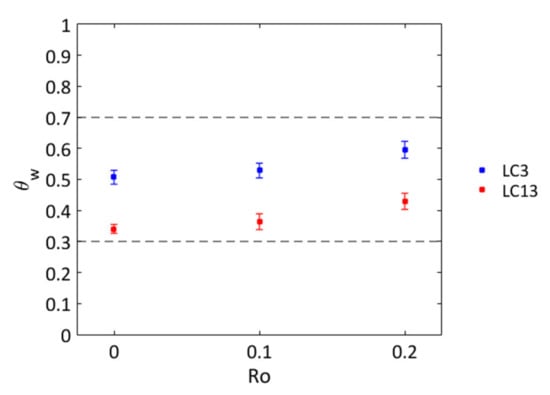
Figure 7.
Averaged dimensionless wall temperature for transient tests.
The HTC is evaluated by solving the one-dimensional heat conduction equation in the wall solid body, starting from an isothermal steady condition between the wall and fluid, followed by a sudden change of the fluid temperature [4]. For a generic flow-temperature evolution, the wall temperature is described solving the heat equation with the help of the Duhamel’s superposition theorem [35]:
Equation (6) is valid as long as the energy diffusion process inside the wall can be assumed as one-dimensional. According to [5], this hypothesis is satisfied by limiting the testing time to the value:
For the current wall thickness and material properties, the maximum allowable testing time is about 170 s—much higher than the experiments duration that was always below 120 s. Equation (6) is numerically solved for by knowing:
- the wall temperature indicated by the LC activation (i.e., a specific temperature is matched to the full intensity of the green colour, as it will be explained in the calibration procedure described in the next subsection);
- the LC activation time (i.e., the elapsed time between the start of the test and the instant at which the green peak is reached);
- the thermo-physical properties of the wall material ;
- the flow-temperature evolution in the entire domain.
Following the approach proposed in [33], the thermocouple readings are spatially interpolated by using the Laplacian diffusion equation in order to determinate the local time-resolved flow temperature. An in-house developed processing software written in Matlab (R2013b, MathWorks, Natick, MA, USA) has been used to perform the heat-transfer computation, namely camera calibration, computation of flow-temperature distribution, image processing in order to get the LC activation time, and solution of Equation (6). The software has been developed over the years, and the details about the implemented algorithm can be found in [14,27].
2.5. Liquid Crystals Calibration
The calibration of the wide-banded LC exploited in the steady-state LCT experiments assesses the relationship between colour hue and temperatures, and it has been performed by means of the well-established temperature gradient approach [36]. The LC are sprayed over a conductive aluminium slab at the ends of which a hot and cold sink are installed. A constant temperature gradient is generated across the slab and monitored through thermocouples that are housed inside the aluminium plate. An image of the active LC is acquired and converted in the hue parameter. This information is then related with the local temperature value obtained by an interpolation of the thermocouple readings. The vision system configuration used for calibration has been set up as similar as possible to the one that has been used for the measurements on the rotating rig. This arrangement prevents from possible calibration errors or issues related to the different viewing angle and illumination.
Narrow-banded LC have been used with the full intensity-matching method in the transient LCT tests. Therefore, the calibration procedure takes charge of the determination of the relationship between the maxima green intensity displayed by the LC and temperature. It has been decided to develop a new methodology that allows evaluating the calibration temperature during a temperature evolution. In this way, hysteresis phenomena can be revealed, and consequently, the proper value can be chosen according to the temperature evolution that occurs during transient tests. A frame made of PMMA holds a 35 × 35 × 4 mm3 copper plate on an aluminium slab through 8 bolts, as illustrated in Figure 8. A removable PMMA window allows the optical accessibility and simultaneously reduces the natural convection. The matt black paint and LC are deposed on the top surface of the copper plate. A water serpentine heat exchanger located just below the aluminium slab performs the required cooling or warming of the copper plate. The heat exchanger is part of a water closed circuit, where the water flow rate is kept constant and a Peltier cell regulates the water temperature at the inlet of the heat exchanger. A thermocouple is situated onto the painted surface to monitor the copper surface temperature, as shown in Figure 8. The calibration facility is designed to have an almost uniform temperature distribution across the copper calibration plate. To verify the plate thermal behaviour, a transient simulation has been performed using Comsol Multiphysics™. The simulation has been carried out for 60 s with a time-step of 0.1 s, with the following boundary conditions: natural convection on all the outer walls and imposed heat flux in the lower face of the copper plate, such to ensure a cooling at a rate of about 0.35 °C/s (which is intentionally above the temperature variation registrable during the current transient LCT tests). During the simulated calibration, the maximum temperature difference inside the copper plate never exceeds 0.03 °C. This evidence confirms that the calibration plate can be considered isothermal and the indication of the surface thermocouple can be used as reference temperature for the LC. The vision system is equivalent to the one used on the rotating facility, and as in that case, the acquisition of temperature and image are synchronized. A region of interest of dimension 10 × 10 pixels has been selected close to the surface thermocouple (see Figure 8) in which the hue of the LC is evaluated. The already mentioned MATLAB routine of the transient data elaboration has been also used in the calibration phase to find the time instants at which the green colour peaks are reached. Then, the temperatures of the plate surface at those instants are associated as calibration temperatures.
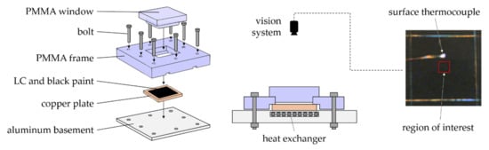
Figure 8.
Sketch of the facility for the calibration through the temperature evolution approach.
2.6. Uncertainty Analysis
The uncertainty analysis has been carried out following the Kline and McClintock’s method [37]. The dimensionless parameters used to identify the test conditions, namely Reynolds and rotation numbers, have been calculated within an uncertainty of 3%.
The uncertainty on HTC in steady-state LCT tests has been determined using the sequential perturbation method described by Moffat [38], or rather, evaluating the sensitivity of the solution with respect to the estimated measurement uncertainties (confidence interval of 95%) of experimental parameters: ±0.4 °C in wall temperature, ±0.2 °C in the fluid temperature, ±0.2 °C in external temperature, ±0.1 V in voltage drops across the Inconel foil, and ±0.5% in electrical resistance of heater element. This has been achieved by running dedicated calculations of the numerical iterative procedure, then applying that information to error propagation. The upper bound for the uncertainty on the heat-transfer results can be assumed equal to 10% for all the tested conditions, and this value applies within the ROI of Figure 5b.
Concerning the transient LCT tests, the sensitivity coefficients necessary to perform the error propagation based on Kline and McClintock’s method cannot be straight forward evaluated because of the analytic form of the Equation (6) used to evaluate the HTC. Therefore, also in this case, sensitivity analyses have been performed [38]. The experimental error sources have been identified and quantified with the following uncertainties: ±5% in material properties, ±0.05 °C in calibration temperature, ±0.2 °C in fluid temperature, and ±0.2 s in activation time. In the present investigation for all the rotating condition and inside the maximum heat-transfer zone, the experimental uncertainties have been estimated up to 3.1% and 6.2% for the LC3 and LC13, respectively. As expected, the LC3 has greater accuracy than the LC13; indeed, the dimensionless wall temperatures of the LC with lower activation temperature are more centred in the range suggested in [34] and previously commented (see Figure 7).
3. Results
3.1. Liquid Crystals Calibrations
The LC employed in the steady-state LCT have been calibrated thanks to the temperature gradient apparatus, as previously described. Multiple calibrations have been performed over time to highlight the potential ageing effect of the LC on the calibration curve [39]. The calibrations have been run the day after the painting of the LC, after two weeks, and after the third week. In each of these days, two calibration curves have been accomplished to check for calibration repeatability, and at least 6 h of waiting time have been interposed between successive calibrations. Since the calibration curves obtained in the same day result overlapped, they are averaged and interpolated by 15th-degree polynomial functions in hue range from 0.05 to 0.65 and are reported in Figure 9. The LC ageing occurs mainly with the attenuation of the colour intensity and, consequently, with the alteration of the calibration curves. For the present case, the ageing does not dramatically affect the hue-temperature relationship within the three investigated weeks. In any case, the wall temperatures have been evaluated using the calibration curve of the first week, since all the heat-transfer measurements have been performed in this period.
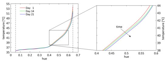
Figure 9.
Hue–temperature calibration curves of R35C7W over time.
Several calibrations have been accomplished over four days for the two LC used in the transient approach (LC3 and LC13). This has been done in order to investigate about possible effects on their activation temperature value due to the experienced temperature time history, including permanence at room temperature (i.e., in the melted state). Calibration values have been obtained by means of the temperature evolution approach during a constant cooling at 0.01 °C/s and a following heating at a rate equal to 0.05 °C/s. The attainable cooling rate is lower by about one order of magnitude than the one in the transient tests. Despite the limited cooling rate, the facility allows pursuing the set aims anyway. In a possible further development, the potential effect of different temperature rates on the calibration values may be studied. The LC has been calibrated also by means of the gradient approach for comparison purpose. The calibration surfaces have been prepared at the same time to ensure consistent performances; furthermore, the investigated surface of the transient test article is prepared at the same time as the calibration specimens. For the sake of clarity, Figure 10 reports only the calibration temperatures obtained for the LC13, since similar trends can be found for the LC3 and analogous considerations can be made about both LC. The outcomes evidence that the calibration values obtained in cooling or heating (negative and positive temperature gradient over time, respectively) follow the same ageing behaviour but with a clear offset. In both cases, calibration value stability is reached from the second day on after LC deposition. Figure 11 reports the averaged calibration data for day 2, 3, and 4; the error bars are associated to the data scattering about the mean values. These graphs clearly highlight the hysteresis phenomena that is observed in the literature but for LC with activation temperatures much higher than the actual ones. More in detail, the cooling calibrations values are lower than heating ones of 0.09 °C for the LC13 and even of 0.16 °C for the LC3. These calibration differences could lead to an error on the heat-transfer evaluation up to about 3%, at least in the present experiments. The commonly adopted temperature gradient approach provides calibration temperatures that are amid the cooling and heating values, with a data scattering that is very wide (about ±0.2 °C), and therefore unacceptable, for the LC at the lowest activation temperature. In summary, the results prove that it is not correct to assume a single calibration temperature for heating, cooling, or steady-state (i.e., temperature gradient) of LC. Consequently, the assigned calibration value has to be obtained with a temperature evolution consistent to that the LC undergo during the tests. In the present work, the inner surface temperatures of the test channel decrease over time, so consequently, the cooling calibration values must be adopted.
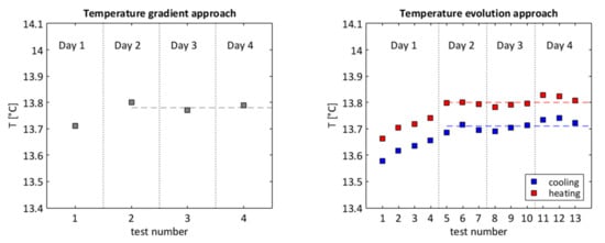
Figure 10.
LC13 calibration values over time.
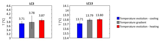
Figure 11.
Averaged calibration values for the LC3 and LC13.
3.2. Heat-Transfer Measurements
Heat-transfer performances are compared and discussed in normalized Nusselt number form through the definition of the enhancement factor:
where is the Nusselt number of a fully developed turbulent flow within a smooth circular section tube by Dittus–Boelter correlation. The exponent is set to 0.4, since the fluid being heated (wall hotter than the fluid) for both LCT approaches. Air thermal conductivity is evaluated at the local bulk fluid temperature. In the transient tests, the fluid temperature changes continuously over time, hence the local fluid temperature at the local activation time has been used as a reference temperature to get fluid properties and also to compute the local buoyancy number. Table 1 recalls the test conditions of the experiments and provides indications of the buoyancy parameters as the averaged value over the 7th and 12th inter-ribs. The test parameters have been selected with the purpose to replicate the same buoyancy number value between the two LCT methodologies.

Table 1.
Averaged buoyancy number over 7th and 12th inter-ribs for all tests conditions.
Figure 12 shows the enhancement factor distributions over the investigated area that have been obtained at the different rotation conditions. It is possible to appreciate that steady-state LCT results are affected by higher data scattering with respect to transient LCT ones. This is a consequence of the noise coming from the nature of the experimental estimation of the surface temperature (i.e., a combination of the colour evaluation and hue-temperature calibration), and the numerical error propagation generated by the numerical iterative process exploited in the data elaboration. The thermal fields of all steady-state LCT tests turn out to be almost symmetrical to the horizontal midline, as expected and already commented (see Section 2.4). The comparison among steady-state and transient approach can be properly conducted in the central inter-rib areas, where the assumptions for the boundary conditions used to process the experimental data for the steady-state tests have negligible effects. The comparison shows that, in static conditions, the distributions are almost the same, and the well-known thermal pattern caused by the rib-roughened surface can be recognized for all the inter-rib regions [2]. A local maximum of is found in correspondence of the reattachment point downstream the obstacle, while regions of lower can be observed upstream of each rib and close to the sidewalls. Immediately downstream of the ribs, very low heat transfer takes place because of a fully separated flow, and indeed, the wall temperature turned out to be out of the activation range of LC for the steady-state test. When the channel goes into rotation, an augmentation of values occurs, as expected in view of the rotational effects and the location of the ribbed wall at the trailing side [40]; anyway, the focus of this contribution is put on the cross-comparison between steady-state and transient approaches and not on the study of the rotational effects. For all rotation conditions, the transient approach delivered for both LC results that are in very good agreement with those from the steady-state approach.
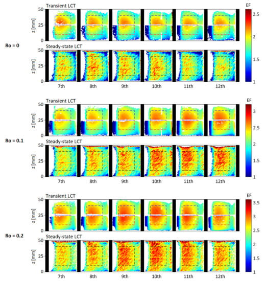
Figure 12.
Enhancement factor distributions.
A more quantitative comparison of the results can be obtained from Figure 13, which reports the profiles collected along the channel length at homologous heights for each rotation condition. For the transient LCT, the data are extracted at z = 20 mm for LC13 and at z = 30 mm for LC3. Two profiles have been extracted at the same locations from the steady-state data and then averaged and compared with those from the transient experiments. The profiles relative to LC3 and LC13 have differences within about 6%, values that fall within the measurement uncertainty estimations. Therefore, the two LC deliver comparable information about heat transfer at different wall temperatures, i.e., at different time during the same tests and, hence, under different fluid temperature histories. This means that the evolution of the rotational effects during the transient tests seems not to have significant consequence on the heat-transfer evaluation, at least for the ranges here investigated. Furthermore, the steady-state profiles are fully comparable with those obtained from the transient LCT under all rotation conditions. A very good congruence among the two LCT approaches can be appreciated about the positions of the heat-transfer maximum (i.e., the location of the flow reattachment downstream the rib). In this way, the steady-state tests attest the right indication of heat transfer achieved by means of the transient tests.
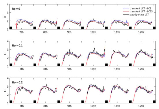
Figure 13.
Enhancement factor profiles.
Another way to point out the validation of the transient tests by the steady-state data can be done considering the area-averaged enhancement factor, . The is calculated for each investigated inter-rib over the evaluation areas that are outlined by dashed lines in Figure 12. The parameter allows making a comparison over a wide portion of the investigated surface, characterized by a large variation of the heat-transfer coefficient, so highlighting possible differences in the outcomes obtained with the two methodologies. For the static channel and for both rotating conditions, the values are practically superimposed, as it is possible to observe in Figure 14. All the inter-ribs have the same behaviour along the channel at , behaviour that changes when the rotation takes place. Indeed, the spatial resolution and the accuracy of the present results is such to allow the detection of rotational effects even on area-averaged data. Going into rotation, the is no longer constant along the channel, a local maximum appears, and it moves upstream as the rotation increases (from the 11th inter-rib at 0.10 to the 9th ÷ 10th inter-rib at 0.20). This phenomenon is already documented in the literature [41], and it is caused by the establishment of flow-coherent structures along the channel length promoted by the rotation. These structures are in continuous development along the channel radial direction, and this development is shortened in space (i.e., it takes less space) if the rotation number is augmented. This heat-transfer development is well-captured by both LCT techniques that deliver values in very good agreement.
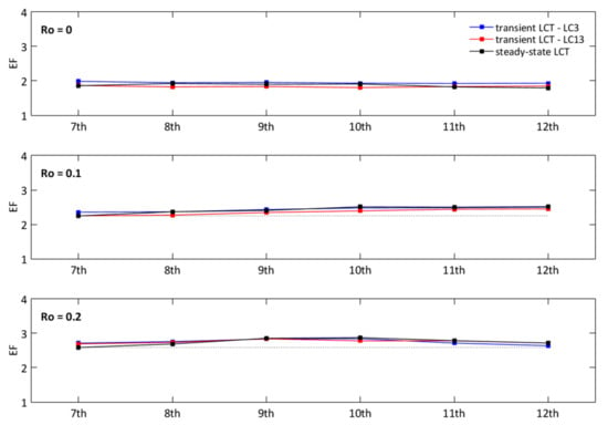
Figure 14.
Averaged enhancement factor on inter-rib areas.
The distributions of the static condition for the transient and steady-state tests are averaged in the z-direction over the 9th inter-rib. Figure 15 offers the comparison of this parameter with the literature, choosing among the available references that report data on geometries and test conditions as close as possible to the present one. The from Mayo et al. [21] is available for test conditions equal to 15,000 and 30,000 and the only difference with the present channel geometry is the cross-section aspect ratio that is equal to 0.9 (present investigation = 1). For the data of Ekkad et al. [22], the is extracted at 12,000 and 60,000 after the 6th rib of the first section of a two-pass ribbed channel with = 0.125 (present investigation = 1). The measurements present similar trends, with values in good agreement if the data at equals 60,000 from [22] are excluded, and there is an agreement in the positions of the maximum of the heat transfer. However, Ref. [22] reported that heat transfer decreases with an increase in Reynolds number, which is not confirmed by [21], where a slight increase of is reported when is raised from 15,000 to 30,000. In addition, the same geometry as in [21] has been used in [23] to perform heat-transfer measurement. The comparison of the maps for the static case from the two contributions shows remarkable differences, the distributions are similar but with reported values much higher for [23]. Even if a very common and simplified cooling channel geometry has been chosen as a case study, the data available in the open literature for validation are pretty much scattered, confirming the complexity to obtain reliable experimental data when heat-transfer measurements are concerned. This evidence justifies the choice to perform dedicated steady-state LCT experiments as a means to providing a reliable reference for the validation of the present transient LCT data.
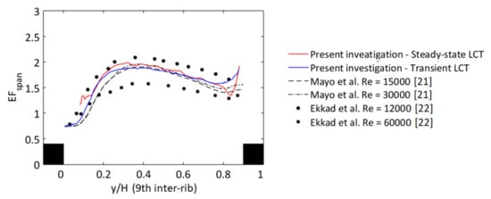
Figure 15.
Span-wise averaged enhancement factor in static condition.
4. Conclusions
This work contributes to the validation of heat-transfer measurements carried out on a rotating cooling channel by means of liquid crystals thermography (LCT) with the transient approach. In this technique, time-dependent rotating effects could affect reliability of the measured heat-transfer performances and their straightforward transfer to the real application. For this reason, the transient LCT has been conducted on a simple case study, and the outcomes have been compared to those achieved through the steady-state LCT technique in which the rotating buoyancy effects are time-stable by definition. The case study is a rotating square cross-section channel with ribs on the trailing side. The investigation has been performed at a fixed Reynolds number of 20,000, in both static and rotating conditions ( 0, 0.10, and 0.20). The different experimental methodologies have led to the design and realization of two test articles, identical in terms of internal geometry but with different technical requirements.
The transient experiments have been conducted, exposing the investigated channel surface to a cold mainstream flow in order to match the direction of the buoyancy effects with those occurring in a real blade cooling application. Consequently, the transient LCT have made use of liquid crystals (LC) with activation range below a standard laboratory temperature. The drawback of this approach is that the LC are in a melted phase for most of their life, in addition to the fact that they are used during a transient thermal regime. This has required an investigation about the best LC calibration procedure to adopt for getting reliable temperature indications out of them with the full intensity-matching method. The calibration temperature of LC has been assessed by means of the common temperature gradient approach and by using a developed facility that allows LC calibration during a temperature evolution. The outcomes of this study prove that calibration values obtained by heating or cooling the LC can differ up to 0.1 °C, and that the temperature gradient approach should not be exploited for the calibration of LC that are used in transient tests. Therefore, in the present contribution, the assigned calibration value has been obtained with a temperature evolution consistent to that which the LC undergo during the tests (i.e., cooling).
In the steady-state LCT, particular attention has been paid in the heat-losses estimation, which have a crucial impact on the experimental accuracy. An iterative numerical thermal analysis has been set up to process the steady-state data. The procedure exploits two numerical models that are built in order to take into account for the conductive and radiative heat losses.
The whole dataset has been analyzed in terms of the enhancement factor (EF) and focus has been put on the cross-comparison between steady-state and transient results by looking at distribution maps, profiles extracted along the channel length, and area-averaged values over the inter-rib domains. For all rotation conditions, the transient approach delivered EF distributions that are in very good agreement with those from the steady-state approach. The well-known thermal pattern caused by the rib-roughened surface can be recognized, and the increasing of the rotation number produces an augmentation of EF values as expected in view of the rotational effects. The shapes of the heat-transfer distributions have been analysed extracting the EF profiles along the channel length. The transient EF profiles are fully comparable with those obtained from the steady-state LCT under all rotation conditions, with a discrepancy that falls within the measurement uncertainty estimations. Moreover, a very good congruence between the two LCT approaches can be appreciated about the positions of the heat-transfer maximum of each inter-rib. The evolution of the heat transfer along the channel have also been pointed out, evaluating the area-averaged EF over each inter-rib domain. For the static case, all the inter-ribs have the same behaviour. Instead, when the channel goes into rotation, several inter-ribs exchange more than others. The maximum area-averaged EF moves upstream as the rotation increases, due to the establishment of flow-coherent structures along the channel length promoted by the rotation. This heat-transfer development is well-captured by both LCT techniques that deliver area-averaged values in very good agreement.
In conclusion, for all rotation conditions, the transient approach delivered results that are in very good agreement with those from the steady-state approach. The results match satisfactorily not only if global values are compared, but also, if local effects are observed. This means that the evolutions of the rotational effects during the transient tests do not have significant consequences on the heat-transfer evaluation, at least for the rotating and buoyancy conditions here investigated, confirming the reliability of the transient LCT methodology here proposed.
Author Contributions
A.L. has collected and processed all the data, handled experimental aspects, and prepared the draft paper. L.C. has continuously contributed in the full process of producing this paper, provided the academic assistance, and revised the manuscript. All authors have read and agreed to the published version of the manuscript.
Funding
This research received no external funding.
Conflicts of Interest
The authors declare no conflict of interest.
References
- Ireland, P.T.; Jones, T.V. Liquid crystal measurements of heat transfer and surface shear stress. Meas. Sci. Technol. 2000, 11, 969–986. [Google Scholar] [CrossRef]
- Rau, G.; Çakan, M.; Moeller, D.; Arts, T. The effect of periodic ribs on the local aerodynamic and heat transfer performance of a straight cooling channel. J. Turbomach. 1998, 120, 368–375. [Google Scholar] [CrossRef]
- Shiau, C.C.; Chen, A.F.; Han, J.C.; Krewinkel, R. Detailed Heat Transfer Coefficient Measurements on a Scaled Realistic Turbine Blade Internal Cooling System. J. Therm. Sci. Eng. Appl. 2019, 12, 31015. [Google Scholar] [CrossRef]
- Pountney, O.; Cho, G.; Lock, G.D.; Owen, J.M. Solutions of Fourier’s equation appropriate for experiments using thermochromic liquid crystal. Int. J. Heat Mass Transf. 2012, 55, 5908–5915. [Google Scholar] [CrossRef]
- Schultz, D.L.; Jones, T.V. Heat Transfer Measurements in Short-Duration Hypersonic Facilities, 1st ed.; North Atlantic Treaty Organization, Advisory Group for Aerospace Research and Development: London, UK, 1973. [Google Scholar]
- Buttsworth, D.R.; Jones, T.V. Radial conduction effects in transient heat transfer experiments. Aeronaut. J. 1997, 101, 209–212. [Google Scholar]
- Wagner, G.; Kotulla, M.; Ott, P.; Weigand, B.; von Wolfersdorf, J. The transient liquid crystal technique: Influence of surface curvature and finite wall thickness. J. Turbomach. 2005, 127, 175–182. [Google Scholar] [CrossRef]
- Von Wolfersdorf, J. Influence of lateral conduction due to flow temperature variations in transient heat transfer measurements. Int. J. Heat Mass Transf. 2007, 50, 1122–1127. [Google Scholar] [CrossRef]
- Kingsley-Rowe, J.R.; Lock, G.D.; Owen, J.M. Transient heat transfer measurements using thermochromic liquid crystal: Lateral-conduction error. Int. J. Heat Fluid Flow 2005, 26, 256–263. [Google Scholar] [CrossRef]
- Ahmed, S.; Singh, P.; Ekkad, S.V. Three-Dimensional transient heat conduction equation solution for accurate determination of heat transfer coefficient. J. Heat Transf. 2020, 142, 51302. [Google Scholar] [CrossRef]
- Waidmann, C.; Poser, R.; von Wolfersdorf, J.; Fois, M.; Semmler, K. Investigations of heat transfer and pressure loss in an engine-similar two-pass internal blade cooling configuration. In Proceedings of the 10th European Conference on Turbomachinery Fluid dynamics & Thermodynamics, Lappeenranta, Finland, 15–19 April 2013. [Google Scholar]
- Domaschke, N.; von Wolfersdorf, J.; Semmler, K. Heat transfer and pressure drop measurements in a rib roughened leading edge cooling channel. J. Turbomach. 2012, 134, 61006. [Google Scholar] [CrossRef]
- Kunstmann, S.; von Wolfersdorf, J.; Ruedel, U. Heat transfer and pressure loss in rectangular one-side-ribbed channels with different aspect ratios. J. Turbomach. 2012, 135, 31004. [Google Scholar] [CrossRef]
- Pagnacco, F.; Furlani, L.; Armellini, A.; Casarsa, L. Gas turbine blades internal cooling: Design, development and validation of a new rig for heat transfer measurements under rotation. In Proceedings of the 12th European Conference on Turbomachinery Fluid dynamics & Thermodynamics, Stockholm, Sweden, 3–7 April 2017. [Google Scholar]
- Lamont, J.A.; Ekkad, S.V.; Alvin, M.A. Detailed Heat Transfer Measurements Inside Rotating Ribbed Channels Using the Transient Liquid Crystal Technique. J. Therm. Sci. Eng. Appl. 2012, 4, 11002. [Google Scholar] [CrossRef]
- Singh, P.; Li, W.; Ekkad, S.V.; Ren, J. A new cooling design for rib roughened two-pass channel having positive effects of rotation on heat transfer enhancement on both pressure and suction side internal walls of a gas turbine blade. Int. J. Heat Mass Transf. 2017, 115, 6–20. [Google Scholar] [CrossRef]
- Singh, P.; Ekkad, S.V. Experimental investigation of rotating rib roughened two-pass square duct with two different channel orientations. In Proceedings of the ASME Turbo Expo, Charlotte, CA, USA, 26–30 June 2017. [Google Scholar] [CrossRef]
- Singh, P.; Ji, Y.; Ekkad, S.V. Multipass Serpentine Cooling Designs for Negating Coriolis Force Effect on Heat Transfer: 45-deg Angled Rib Turbulated Channels. J. Turbomach. 2019, 141, 71003. [Google Scholar] [CrossRef]
- Singh, P.; Ji, Y.; Ekkad, S.V. Multi-Pass Serpentine Cooling Designs for Negating Coriolis Force Effect on Heat Transfer: Smooth Channels. J. Turbomach. 2019, 141, 71001. [Google Scholar] [CrossRef]
- Waidmann, C.; Poser, R.; Nieland, S.; Von Wolfersdorf, J. Design of a rotating test rig for transient thermochromic liquid crystal heat transfer experiments. In Proceedings of the Open archives of the 16th ISROMAC 2016, Honolulu, HI, USA, 10–15 April 2016. [Google Scholar]
- Mayo, I.; Lahalle, A.; Gori, G.L.; Arts, T. Aerothermal characterization of a rotating ribbed channel at engine representative conditions-part II: Detailed liquid crystal thermography measurements. J. Turbomach. 2016, 138, 101009. [Google Scholar] [CrossRef]
- Ekkad, S.V.; Han, J.-C. Detailed heat transfer distributions in two-pass square channels with rib turbulators. Int. J. Heat Fluid Flow 1997, 40, 2525–2537. [Google Scholar] [CrossRef]
- Mayo, I.; Arts, T.; El-Habib, A.; Parres, B. Two-Dimensional Heat Transfer Distribution of a Rotating Ribbed Channel at Different Reynolds Numbers. J. Turbomach. 2014, 137, 31002. [Google Scholar] [CrossRef]
- Abdullah, N.; Abu Talib, A.R.; Mohd Saiah, H.R.; Jaafar, A.A.; Mohd Salleh, M.A. Film thickness effects on calibrations of a narrowband thermochromic liquid crystal. Exp. Therm. Fluid Sci. 2009, 33, 561–578. [Google Scholar] [CrossRef]
- Anderson, M.R.; Baughn, J.W. Hysteresis in liquid crystal thermography. J. Heat Transf. 2004, 126, 339–346. [Google Scholar] [CrossRef]
- Kakade, V.U.; Lock, G.D.; Wilson, M.; Owen, J.M.; Mayhew, J.E. Accurate heat transfer measurements using thermochromic liquid crystal. Part 1: Calibration and characteristics of crystals. Int. J. Heat Fluid Flow 2009, 30, 939–949. [Google Scholar] [CrossRef]
- Pagnacco, F.; Furlani, L.; Armellini, A.; Casarsa, L.; Davis, A. Rotating heat transfer measurements on a multi-pass internal cooling channel-I rig development. In Proceedings of the ASME TE16, Seoul, Korea, 13–17 June 2016. [Google Scholar] [CrossRef]
- Measurement of Fluid Flow by Means of Pressure Differential Devices Inserted in Circular Cross−Section Conduits Running Full–Part 2: Orifice Plates. ISO 5167-2. 2003. Available online: https://www.iso.org/standard/30190.html (accessed on 11 September 2020).
- Farina, D.J.; Hacker, J.M.; Moffat, R.J.; Eaton, J.K. Illuminant invariant calibration of thermochromic liquid crystals. Exp. Therm. Fluid Sci. 1994, 9, 1–12. [Google Scholar] [CrossRef]
- Lucas, M.L.; Ireland, P.T.; Wang, Z.; Jones, T.V. Fundamental Studies of Impingement Cooling Thermal Boundary Conditions. In Proceedings of the 80th Propulsion and Energetics Panel Symposium AGARD, Antalya, Turkey, 12–16 October 1992. [Google Scholar]
- Çakan, M. Aero-Thermal Investigation of Fixed Rib-Roughened Internal Cooling Passages. Ph.D. Thesis, Université Catholique de Louvain and von Karman Institute for Fluid Dynamics, Louvain, Belgium, 2000. [Google Scholar]
- Scienza e Tecnologia dei Materiali. Available online: http://www.nanofun.net/ (accessed on 24 July 2020).
- Poser, R.; von Wolfersdorf, J.; Lutum, E. Advanced evaluation of transient heat transfer experiments using thermochromic liquid crystals. In Proceedings of the 7th ETC, Athens, Greece, 5–9 March 2007. [Google Scholar]
- Yan, Y.; Owen, J.M. Uncertainties in transient heat transfer measurements with liquid crystal. Int. J. Heat Fluid Flow 2002, 23, 29–35. [Google Scholar] [CrossRef]
- Metzger, D.E.; Larson, D.E. Use of melting point surface coatings for local convection heat transfer measurements in rectangular channel flows with 90-deg turns. J. Heat Transf. 1986, 108, 48–54. [Google Scholar] [CrossRef]
- Cukurel, B.; Selcan, C.; Arts, T. Color theory perception of steady wide band liquid crystal thermometry. Exp. Therm. Fluid Sci. 2012, 39, 112–122. [Google Scholar] [CrossRef]
- Kline, S.J.; McClintock, F.A. Describing Uncertainties in Single-Sample Experiments. Mech. Eng. 1953, 75, 3–8. [Google Scholar]
- Moffat, R.J. Describing the uncertainties in experimental results. Exp. Therm. Fluid Sci. 1988, 1, 3–17. [Google Scholar] [CrossRef]
- Wiberg, R.; Lior, N. Errors in thermochromic liquid crystal thermometry. Rev. Sci. Instrum. 2004, 75, 2985–2994. [Google Scholar] [CrossRef]
- Coletti, F.; Jacono, D.L.; Cresci, I.; Arts, T. Turbulent flow in rib-roughened channel under the effect of Coriolis and rotational buoyancy forces. Phys. Fluids 2014, 26, 45111. [Google Scholar] [CrossRef]
- Pascotto, M.; Armellini, A.; Mucignat, C.; Casarsa, L. Coriolis effects on the flow field inside a rotating triangular channel for leading edge cooling. J. Turbomach. 2013, 136, 31019. [Google Scholar] [CrossRef]


© 2020 by the authors. Licensee MDPI, Basel, Switzerland. This article is an open access article distributed under the terms and conditions of the Creative Commons Attribution (CC BY) license (http://creativecommons.org/licenses/by/4.0/).