Article

Time Series Forecasting with Multi-Headed Attention-Based Deep Learning for Residential Energy Consumption

Department of Computer Science, Graduate School of Artificial Intelligence, Yonsei University, Seoul 03722, Korea
*
Author to whom correspondence should be addressed.
Energies 2020, 13(18), 4722; https://doi.org/10.3390/en13184722
Submission received: 7 June 2020 / Revised: 27 August 2020 / Accepted: 2 September 2020 / Published: 10 September 2020
(This article belongs to the Special Issue Time Series Forecasting for Energy Consumption)

Abstract

:
Predicting residential energy consumption is tantamount to forecasting a multivariate time series. A specific window for several sensor signals can induce various features extracted to forecast the energy consumption by using a prediction model. However, it is still a challenging task because of irregular patterns inside including hidden correlations between power attributes. In order to extract the complicated irregular energy patterns and selectively learn the spatiotemporal features to reduce the translational variance between energy attributes, we propose a deep learning model based on the multi-headed attention with the convolutional recurrent neural network. It exploits the attention scores calculated with softmax and dot product operation in the network to model the transient and impulsive nature of energy demand. Experiments with the dataset of University of California, Irvine (UCI) household electric power consumption consisting of a total 2,075,259 time-series show that the proposed model reduces the prediction error by 31.01% compared to the state-of-the-art deep learning model. Especially, the multi-headed attention improves the prediction performance even more by up to 27.91% than the single-attention.

1. Introduction

According to the World Energy Outlook 2019, the International Energy Agency (IEA) pointed out that the energy demand will rise by 1.3% each year to 2040 with unrestrained planning by further efforts to improve efficiency [1]. The residential power consumption sector, which is a major factor that accounts for 27% of global electricity consumption [2], provides an ideal testbed for power demand prediction and analysis with a relatively limited and closed environment. The machine learning approach including the deep learning algorithms is convincing as a premise for power supply planning due to its non-linear learning capability [3].
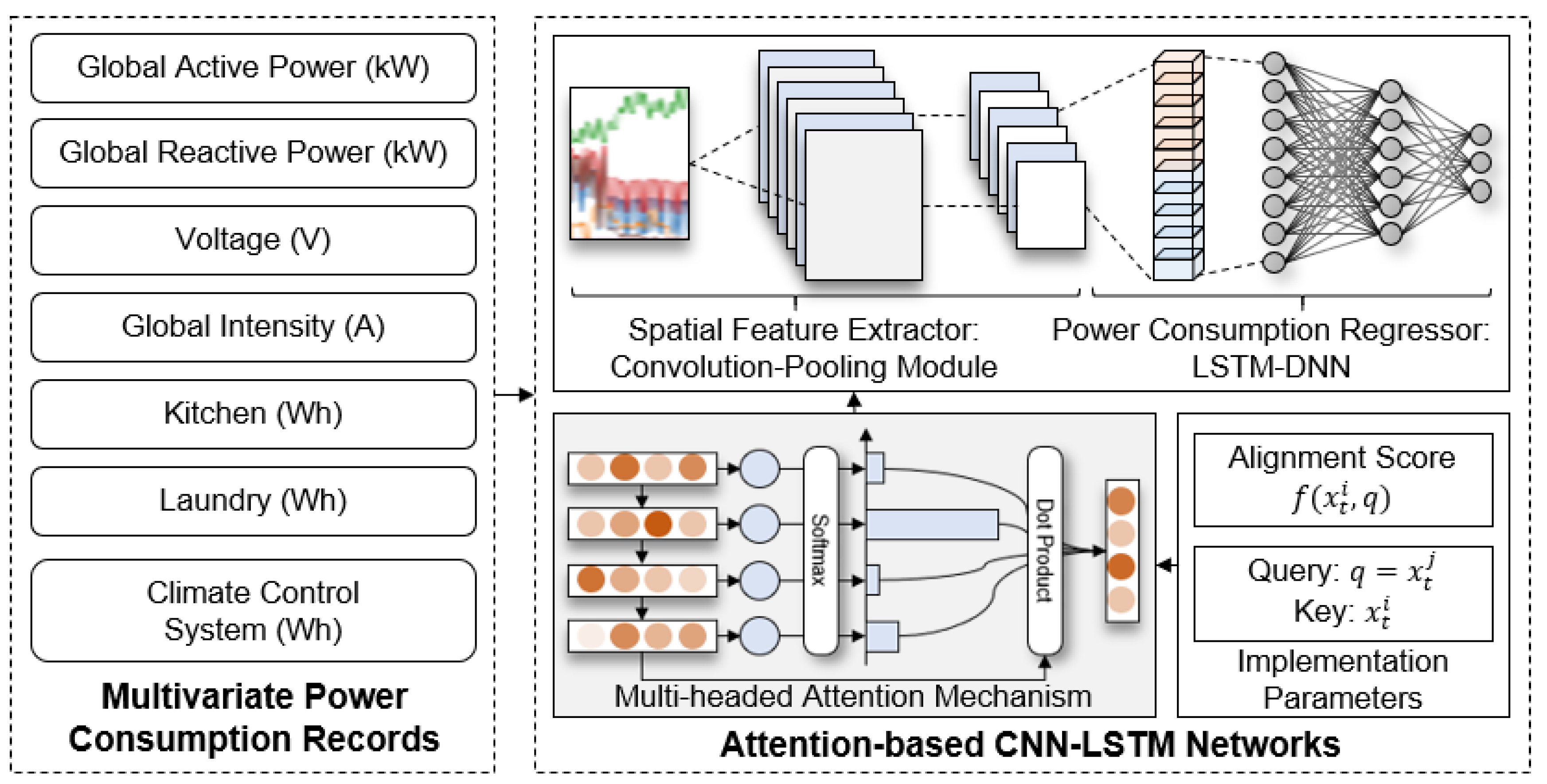
Residential power consumption prediction is defined as a multivariate time series prediction problem [4]. As depicted in Figure 1, the differentiated features from sensor-level signals consisted of energy consumption attributes are extracted to predict the power consumption levels with the prediction model [5]. The process of predicting the future power demand from the historical power consumption with the other power attributes is essential in the field of energy management system (EMS) including the recently noted smart grid services. The main issue at the planning stage of the plan-do-check-act operation cycle [6] in traditional EMS is modeling the nature of energy consumption, which is limited to naive time-series models such as linear regression.
In the domain of energy, machine learning aims at exploiting a database generated with the historical data of all the clients and predicting the future energy demand. Various regression techniques, including autoregressive integrated moving average [7] and support vector regressor [8], which are representative methods for the energy prediction, successfully model the long-term behavior of end-users and improve the prediction accuracy. Yet, in the prediction task under high-temporal resolution conditions [9] aimed at modeling the short-term behaviors that expose the behavioral patterns, a more complex and practical time series modeling method is required.
The power prediction models based on deep learning which achieved the highest performance so far [10], on the other hand, encounter two major hurdles: One is the multicollinearity between active power consumption patterns and other power attributes [11,12], and the other is the transient and impulsive nature of power consumption mainly occurring from the usage of electronic products. Although the convolution operation to learn the filter to extract the local correlation has been devised, the simultaneous or exclusive usage of power consuming facilities that have a critical effect on the active power cause the performance degradation of the deep learning models. Specifically, it is known that the state-of-the-art models that do not focus on modeling the multivariate and impulsive properties have their performance degradation in energy peaks.
The dataset of UCI household electric power consumption consisting of a total 2,075,259 time-series and seven variables is a representative example of the typical difficulty of modeling between the active power and the power consuming facilities. Figure 2 shows the correlation between the active, reactive power, voltage, intensity and three sub metering attributes. With the color of the graph is shown the active power level grouped into three stages, the existing deep learning-based models have the limitation to hardly concentrate the control facility to predict power consumption.
In this paper, we propose a deep learning model based on multi-headed attention to model the local connectivity between electric attributes and active power with the learnable feature extraction of convolution and weighting mechanism in time-series modeling [13,14]. The key idea is to extract the features from the multivariate electric attributes with the convolution operation, perform time-series modeling of the power spectrum with the gating operation, and effectively predict the transient and impulsive values of power consumption with multi-headed attention that performs probabilistic data localization based on the softmax operation. Taken together, our hypothesis of the proposed method is that the weighting function of attention can model the short-term patterns of time-series electricity data including the energy peaks. We will show that the multi-headed attention selectively extracts the power consumption patterns to cope with the challenge mentioned previously. To the best of our knowledge, this is the first attempt that multi-headed attention is incorporated to predict power consumption. The main findings of this research can be summarized as follows:
  • The multi-headed attention works well for modeling the short-term patterns of time-series data, resulting in the best deep learning model for predicting the energy demand.
  • The class activation map appropriately visualizes how the proposed method forecasts the energy demand from the time-series data.
The remainder of this paper is organized as follows. In Section 2, we review the previous power consumption models based on deep learning and clarify the contributions of this paper by discussing the differences between them. In Section 3 we illustrate how the electric attributes are selectively extracted by the deep learning model with multi-headed attention. The performance of the model is evaluated in Section 4 through various experiments, including the visualization of multi-headed attention vectors and comparison with recent models based on deep learning. Finally, Section 5 concludes the paper with some discussion of future directions.

2. Related Works

In this section, we review the relevant models based on deep learning for forecasting energy consumption. According to the similarities of the fields and the techniques used, we present the traditional signal processing methods as well as the power prediction studies based on deep learning. Table 1 summarizes the significant studies of the last five years on predicting power consumption in terms of the feature extraction and time series modeling. Most of the methods before the inception of deep learning focused on the issue of time series modeling based on the symbolic-dynamic approach [15,16]. Due to the limitations that slight shifts along the time axis causing a large distance between the two time series, Lin et al. extracted and modeled the rotation-invariant symbols and constructed the bag-of-patterns [17].
Meanwhile, the superiority claims by the power demand models based on machine learning encountered a major hurdle: the methods are evaluated for short-term forecasting horizons and do not consider medium and long-term ones [7]. In order to build time-invariant features and perform the non-linear mapping for predicting the power consumption, Tso and Yau presented a neural network and compared the performance with existing prediction methods based on the rules and symbols [18]. Among the power demand forecasting methods based on machine learning such as the autoregressive integrated moving average (ARIMA) [7] and decision tree [8], the neural network achieved the best performance, and its non-linear mapping capability attracted much attention [19]. In particular, combining the approach of machine learning algorithms like the ensemble of recurrent neural network and support vector regressor [20] improved the accuracy and the stability of power demand prediction.
The deep learning models, including the long short-term memory (LSTM) which can learn temporal gating functions and the convolutional neural network (CNN) which can extract local correlation between power spectrums, are making remarkable achievements in the field of energy consumption forecasting and energy pattern classification [10]. Moreover, designed as a probabilistic approach using CNN and LSTM layers as building blocks, autoencoder (AE) [24] and adversarial learning models like generative adversarial network (GAN) [33] indirectly demonstrate the popularity and possibility of deep learning for power consumption prediction.
However, electricity demand forecasting is a difficult task due to the characteristics that demand time-series exhibit. The characteristics include the non-constant mean and variance, calendar effects, multiple periodicities, high volatility, jumps, et cetera. Mocanu et al. introduced a stochastic pretraining stage into the power consumption prediction with a neural network and evaluated it under various temporal conditions [21]. Restricted Boltzmann machine (RBM) is a representative neural network model of unsupervised learning that aims to minimize the divergence of the Kullback–Leibler divergence between the layers [34]. The stacked RBM is suitable for learning the prior distribution from the power consumption data and has been contributed significantly to improving the prediction performance. Marino et al. and Kong et al. attempted to predict the power consumption by using the recurrent neural network (RNN) with LSTM designed for time series modeling, and verified that the feasibility of a neural network with memory cell could significantly improve the prediction performance [22,23].
To account for the different characteristics of the demand-series, recently, researchers suggested optimization methods for forecasting models. The optimization of deep learning architecture or loss function has been performed for the remarkable performance improvement in various domains. Li et al. introduced the autoencoder before the time-series modeling to extract multivariate features [24], and the RNN with pooling operation to selectively update the gradient [30]. A method of optimizing the time lag parameters, a critical factor for prediction performance, by genetic algorithm (GA) was also introduced [31]. Furthermore, the optimization of the power prediction model with particle swarm optimization (PSO), which has faster convergence and larger exploration of searching the space than GA, attracted the attention by outperforming the performance of existing deep learning models [29]. In addition, studies have proceeded to optimize or develop the loss functions, such as adaptation of quantile loss function into neural networks [27,32].
From the relevant studies on deep learning applications to predicting energy consumption, it is obvious that this area serves as a competitive platform for various deep learning techniques. In this paper, we present another model based on the multi-headed attention on top of the most superior model based on CNN-LSTM (convolutional neural network-long short-term memory).

3. Convolutional Recurrent Neural Network with Multi-Headed Attention

In this section, we describe the architecture of the CNN-LSTM network with multi-headed attention that extracts the spatiotemporal features and models the power consumption from the power spectrum. Two major components of the conventional power prediction model are adopted and modified with end-to-end neural network architecture. Here, the multi-headed attention is implemented with softmax and dot product operation to model the transient and impulsive values of electricity demand.

3.1. Structure Overview

The main objective of the method is to forecast the electricity demand using CNN-LSTM network. We incorporate the multi-headed attention mechanism and formulate it with the function ϕ ( ) that extracts the spatiotemporal features and predicts the future energy demand. Since there is a complex non-linear mapping expressed by stacking the multiple layers, we adopt a direct forecast strategy [35] that avoids the accumulation of bias in the recursive strategy. The direct forecast strategy is formulated with direct model ϕ h and its parameter Θ h :
y ^ t = ϕ h ( X t h ω ; Θ h ) + e t , h
where X t h ω = [ R t h , , R t h ω ] with time lag ω , Θ h = [ ψ h , θ h ] is the model parameter for horizon h where ψ h is a set of hyperparameters and θ h is a set of parameters, and e t , h is the forecast error of the model ϕ h . The electricity demand forecaster predicts h   -step ahead, and we verify the model under various conditions of {1-min, 10-min, ..., 1-day, 1-week} in Section 4. The input element R t of the sequence of the power attribute vector is composed of global active power, reactive power, voltage, intensity, and three sub-meterings.
It is well known that the convolutional recurrent neural networks have the advantages represented by data-driven filter learning focused on extracting spatiotemporal features in the field of signal processing, including predicting the power consumption [10,36]. Figure 3 illustrates the overall architecture of the CNN-LSTM with the multi-headed attention for predicting power consumption. The proposed model for predicting the future power consumption from the input power data consists of two major stages.
First, the data preprocessing stage defines the hyperparameters required for training the CNN-LSTM model. Min–max normalization per each power attribute and the sliding-window, one of the most common preprocessing methods, are performed before defining the hyperparameter. The sliding-window is defined by the length of the input signal ω called time lag with the stride parameter τ that determines the amount of overlapping time steps. The power consumption data are sampled with each period, and the proposed method is verified under the temporal resolution R t of 1, 15, 30, 45, and 60 min, 1 day, and 1 week, respectively.
Second, the modeling stage adjusts the weights of CNN-LSTM model according to the hyperparameters defined. To extract spatiotemporal features from the power spectrum, we construct a convolution-pooling operation that models the hidden correlations between power attributes [37], and the gating operation applied to a recurrent memory cell that models the temporal relations from time-series data [38]. Meanwhile, the multi-headed attention designed to interpret the activation value as a probability and construct a correlation matrix with itself is implemented as a layer of the CNN-LSTM model to be placed between each convolutional and recurrent layer [39]. In addition, the class activation map (CAM) is put in the last convolutional layer for the analysis of the network outputs, which can localize the receptive field by summing the weights of CNN’s top-most feature maps [40].

3.2. Convolutional Recurrent Neural Networks

The major hurdle in modeling the power consumption with neural regressor lies in extracting the spatiotemporal features from the limited consumption samples [41]. We construct the CNN and LSTM for learning the features from the time-series power consumption data. The two deep learning models are combined in a sequential manner, while maintaining the complementary relations from spatiotemporal features.
The convolution ϕ c ( ) and the pooling operation in CNNs, which have been successfully applied in the field of the signal processing, are suitable to model the sequence of power consumption and extract the features using local connectivity between windowed signals. The convolution operation is known to reduce the translational variance between features [42] and preserves the spatial relationship between power attributes by learning filters to extract the hidden correlations. Given the t   -th time step, the sequence of the convolutional operation is applied using m × 1 sized filter W with the a   -th node in the l   -th layer and τ   -th element in sequence of the power attributes R τ :
ϕ c l ( X t ) = [ a = 0 m 1 W a l 1 R τ ] τ = 1 t ω
Because the dimension of the output vector that has been distorted and copied by the convolution operation ϕ c ( ) is increased by the number of convolution filters, the summary statistic from nearby node activations is extracted from ϕ p ( ) by a max-pooling operation. Pooling refers to a dimension reduction process used in CNN in order to impose the capacity bottleneck and facilitate faster computation [43]. The max-pooling operation has effects on feature selection and dimensionality reduction under k × 1 sized area with pooling stride. The proposed 1D convolution-pooling operation aims to extract the spatial features from the power spectrum per attributes and deliver the series of encoded vectors to the following LSTM. The spatial features extracted by convolution-pooling function ϕ c contain the time-series information of the window size ω according to the sliding-window preprocessing. The key idea of LSTM is adapting the gating operation which is composed of input gate, forget gate, and output gate o t and producing the encoded vector ϕ L ( ) with the cell state c t and the hidden value h t at the time step t :
ϕ L ( ) = h t = o t t a n h ( c t )
where denotes the element-wise product and b denotes bias term. After the spatiotemporal features are extracted by CNN-LSTM, the typical multi-layer perceptron (MLP) is used to complete the regression function ϕ ( ) with activation function σ and weight matrix W l :
ϕ l ( X t ) = σ ( W l ϕ L l 1 ( ϕ c l 2 ( X t ) ) + b l )
where a linear activation function is used in the last layer of MLP so that the output scalar value y ^   is interpreted as a power prediction. The CNN-LSTM regressor is updated by the backpropagation algorithm with gradient descent optimization, by minimizing the loss function represented by mean squared error (MSE) where n denotes the number of observations:
L M S E = 1 n i = 1 n ( y i y ^ i ) 2

3.3. Multi-Headed Attention

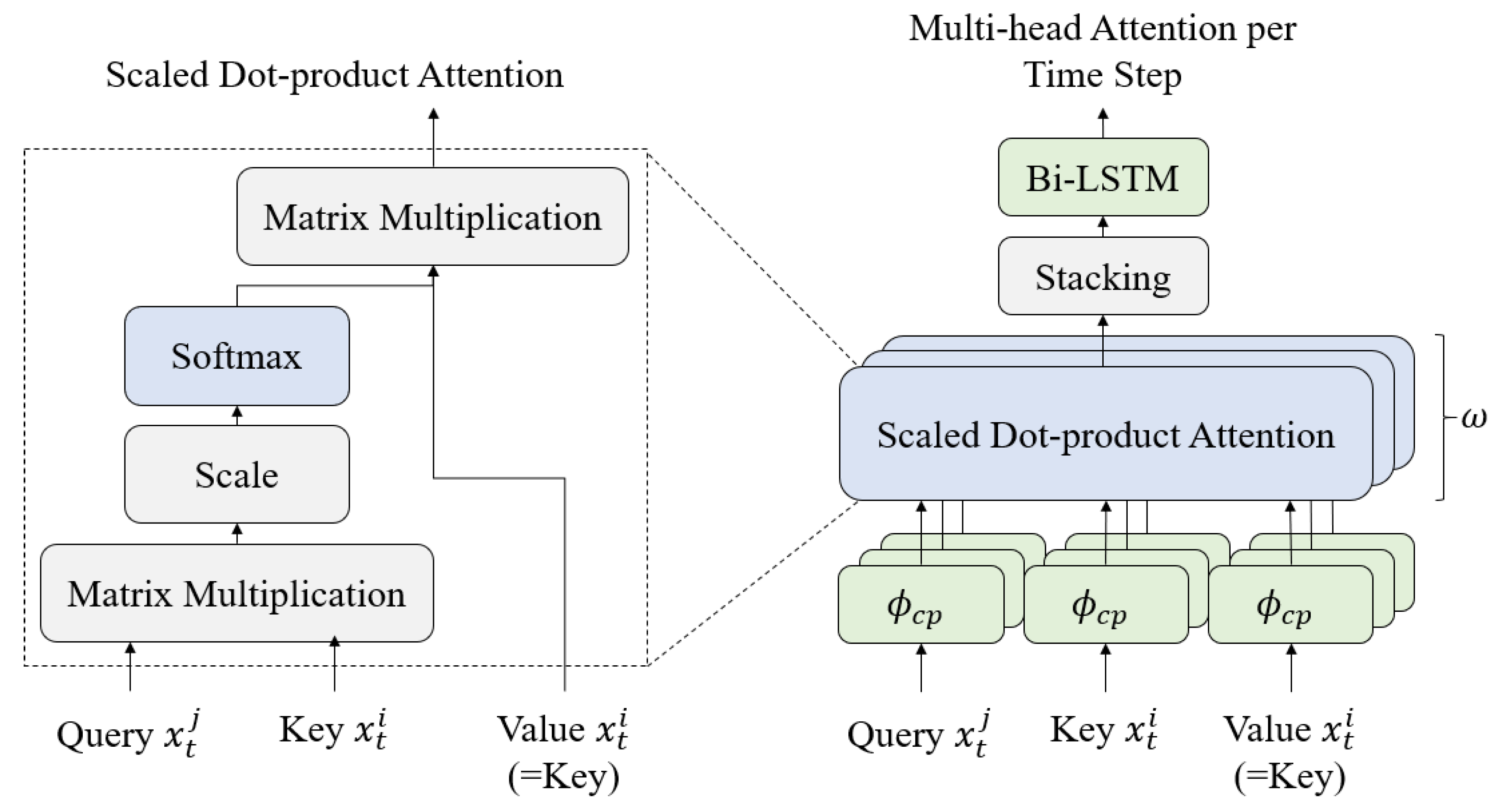
Attention is used to compute an alignment score between elements from two sources [44,45]. Intuitively, the attention mechanism is formulated as an operation to calculate the similarity between query and key, and to extract the value related to the query as a weighted sum. Given the time step t of the window X t ω = [ R t , , R t ω ] and the spatiotemporal feature vector representation of a query q , attention computes the alignment score by a compatibility function f ( R t , Q ) which measures the correlation between R t and Q . The alignment score vector A t = [ f ( R τ , Q ) ] τ = t t ω consists of a series of correlations between the elements of query and key measured by the compatibility function:
A t = [ f ( R τ , Q ) ] τ = t t ω
The compatibility function is interpreted as a probability distribution p ( z | X ,   Q ) by a softmax operation, with the indicator variable z as defined as follows:
p ( z | R t , Q ) = s o f t m a x ( A t )
The correlation between the query Q and the key expressed on the scale of [0,1] can be expressed as a random variable defined in the following equations as the attention score s , and can be written as the expectation of the energy consumption sampled according to its importance:
p ( z = t | Q ) = e x p ( f ( R t , Q ) ) τ = t t ω e x p ( f ( R τ , Q ) )
  S t = τ = t t ω p ( z = τ | R t , Q ) = Ε t ~ p ( z | R t , Q ) ( R t )  
The compatibility function f is commonly used as an additive or multiplicative operation. The function f is implemented as the multiplicative (dot-product) operation that guarantees memory-efficient and fast convergence when considering the characteristics of the power consumption data of huge instances, with the spatiotemporal feature encoding function ϕ c p ( ) defined in Section 3.2:
f ( R t , Q ) = ϕ c p l ( R t ) ϕ c p l ( Q )
The attention mechanism is implemented as the deep learning layers; the attentive layer is placed between the modeling steps of the power spectrum and the time series. The attention layers are suitable for modeling the sudden increase in the usage of the power facilities which were difficult to predict by conventional deep models for predicting the power consumption. Self-attention is a special case of the attention: it replaces query Q with a source signal X t . The single-attention mechanism intuitively performs dot-product on itself encoded by the convolution-pooling operation, and as the effect of obtaining the covariance between spatiotemporal feature vectors.
The proposed multi-headed attention, on the other hand, is an extension of the attention mechanism, which holds multiple attention in a single window and performs better than single-headed attention [45]. Figure 4 shows the multi-headed attention. Instead of computing a single scalar score f ( X t ,   X t ) for each time step, we define the output of compatibility function f with the vector of the same length as X t . Z k denoting the alignment score from the compatibility function. Since we have expanded the dimension of the attention vector into [ f ( R τ , Q ) ] τ , we can formalize the importance weight vector P k t for the element of the power attribute or encoded feature k in each step t :
P k t = p ( Z k = i | R t , Q )
  S t = [ τ = t t ω P k τ R t   k τ ] k = 1 d e = [ Ε t ~ p ( Z k | R t , Q ) ( R t k t ) ] k = 1 d e  

4. Experimental Results

In this section, we present how the CNN-LSTM with multi-headed attention predicts the power consumption and evaluate the performance with 10-fold cross-validation in terms of prediction error, which is followed by quantitative comparison with the relevant deep learning models.

4.1. Dataset and Implementation

We validate the proposed CNN-LSTM with multi-headed attention on the dataset of UCI household electric power consumption [46]. As shown in Table 2, the data were collected as approximately 2.07 million multi-channel sensors recording the household power consumption from December 2006 to November 2010, and the attributes include global active power (GAP), global reactive power (GRP), voltage, intensity, and additional three sub meterings. The data are normalized and processed in a sliding-window with time lag parameter ω . The prediction model receives the seven attributes under the time resolution condition and produces the GAP of the next time step.
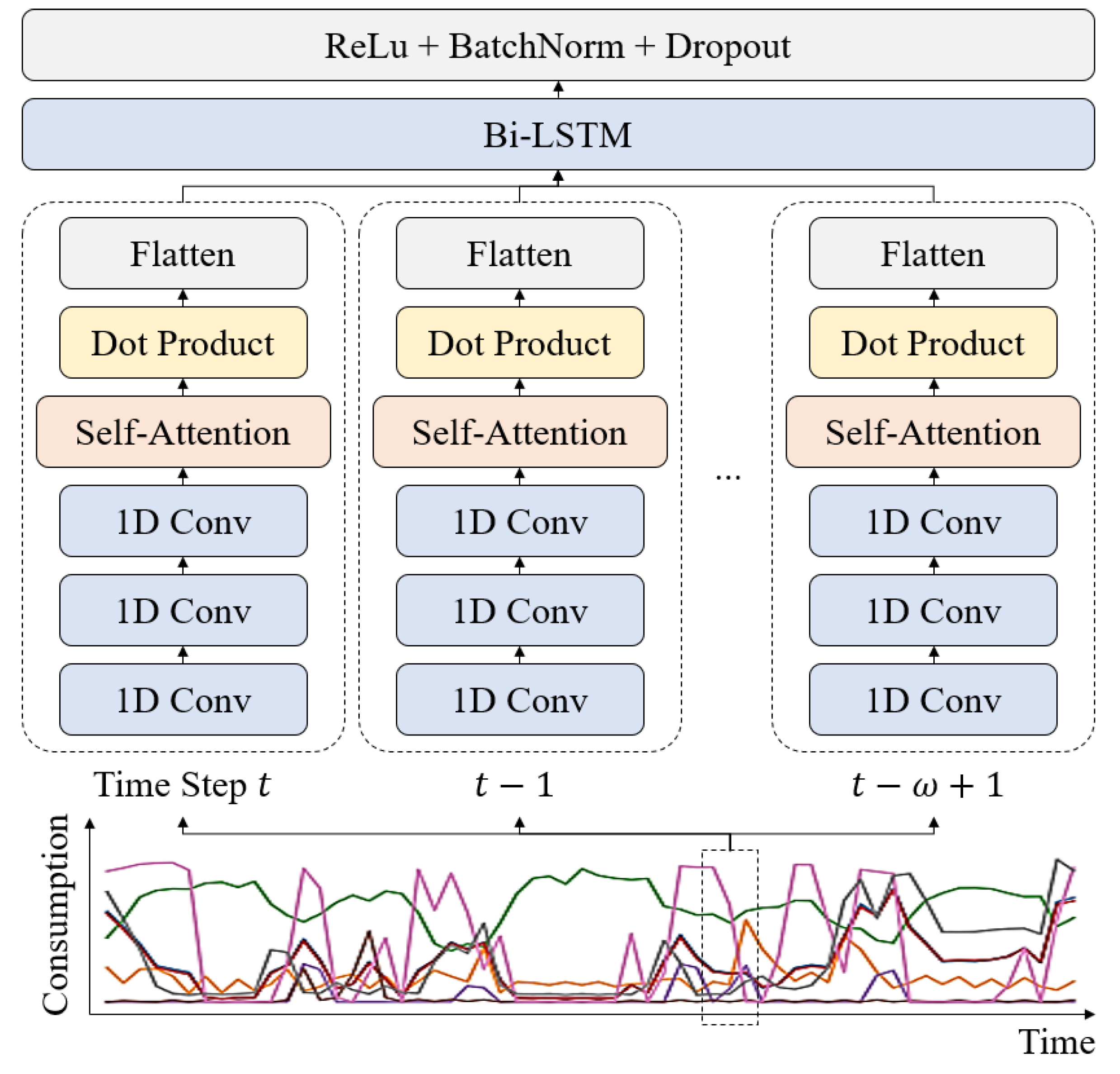
The architecture of CNN-LSTM can be modified variously according to the number of stacked convolution-pooling and LSTM layers, as well as the number of convolutional filters, the kernel size and the number of the nodes in LSTMs. Given that typical deep learning models require an optimization process, it is essential to adjust and optimize the hyperparameters. The hyperparameters of the proposed model are determined by the intuition from the statistics of energy consumption as well as a through empirical study of iterative optimization summarized in Table 3. Figure 5 shows the overall architecture of the proposed model, where the time-distributed convolution-pooling layers, the self-attention, and LSTM layers are depicted. The spatiotemporal features from the power consumption data at each time step are exclusively extracted from time-distributed convolution and LSTM layers, respectively.

4.2. Power Consumption Prediction Performance

Figure 6 compares the results of the prediction performance for the machine learning models including the convolution neural network and LSTM neural network. The proposed model designed to selectively model the spatiotemporal features has achieved the error reduction of 21.82%, compared to the conventional CNN-LSTM neural network. The evaluation is based on the mean squared error (MSE) for measuring the errors in Euclidean space:
M S E = 1 n i = 1 n ( y t y ^ t ) 2 = 1 n i = 1 n ( y t ϕ ( X t ) ) 2
We further evaluate the proposed model in various time resolutions of 1, 15, 30, 45, and 60 min, 1 h, 1 day, and 1 week in Table 4. Each MSE is the result of the 10-fold cross validation. We compare machine learning methods for power demand forecasting published in the last two years. The prediction error is the highest at the unit time of 45 min and 1 h, and sometimes the performance degradation occurs due to the loss of short-term temporal features that might disturb the long-term temporal modeling. Considering that the end-user’s long term behavior is reflected as a trend at low temporal resolution, the smoothing strategy is effective. It is known that the autoregressive integrated moving average (ARIMA) can model the overall trend of the time-series based on the moving average operation. As expected, the advantages of ARIMA emerge in the long period of 1W and 1D, and nonlinear mapping methods such as support vector regressor (SVR) and neural networks alleviate errors in a short period of 1H and 1M. The proposed method achieves the best performance in all temporal resolutions against the latest machine learning methods [7,8] and deep learning method [10].
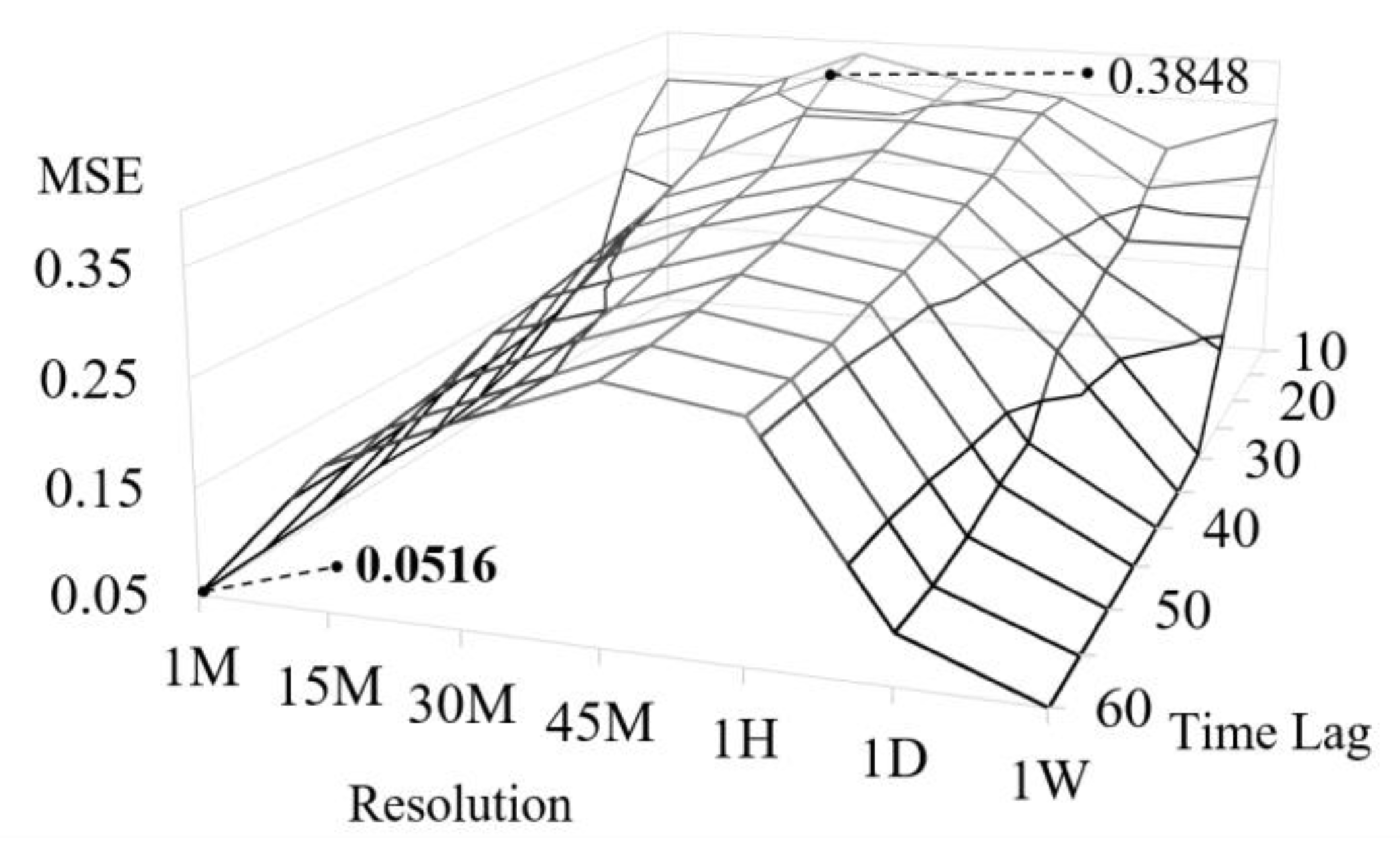
We confirm the effect of changes in time lag parameter ω . Figure 7 shows the MSE performance by iterative evaluations according to the temporal resolution and the time lag. As in the previous experimental results, it is observed that the prediction error considerably increases and yields 0.3848 MSE in the condition of 45 to 60 min, and the prediction error similarly increases regardless of the resolution with a short time lag.

4.3. Effects of Multi-Headed Attention

For a thorough comparison, in addition to the neural networks proposed in previous works for energy prediction, we implement four additional neural networks and compared the prediction errors in Table 5. The scalability of the multi-headed attention can be evaluated by improving the different neural network architectures. It can be seen that the multi-headed attention improves the performance for power prediction in all cases. Interestingly enough, the single-attention significantly improves the performance of 2D-CNN, implying that a filter of extracting temporal features within a 2D convolution filter is appropriately learned from the local connectivity of time steps.
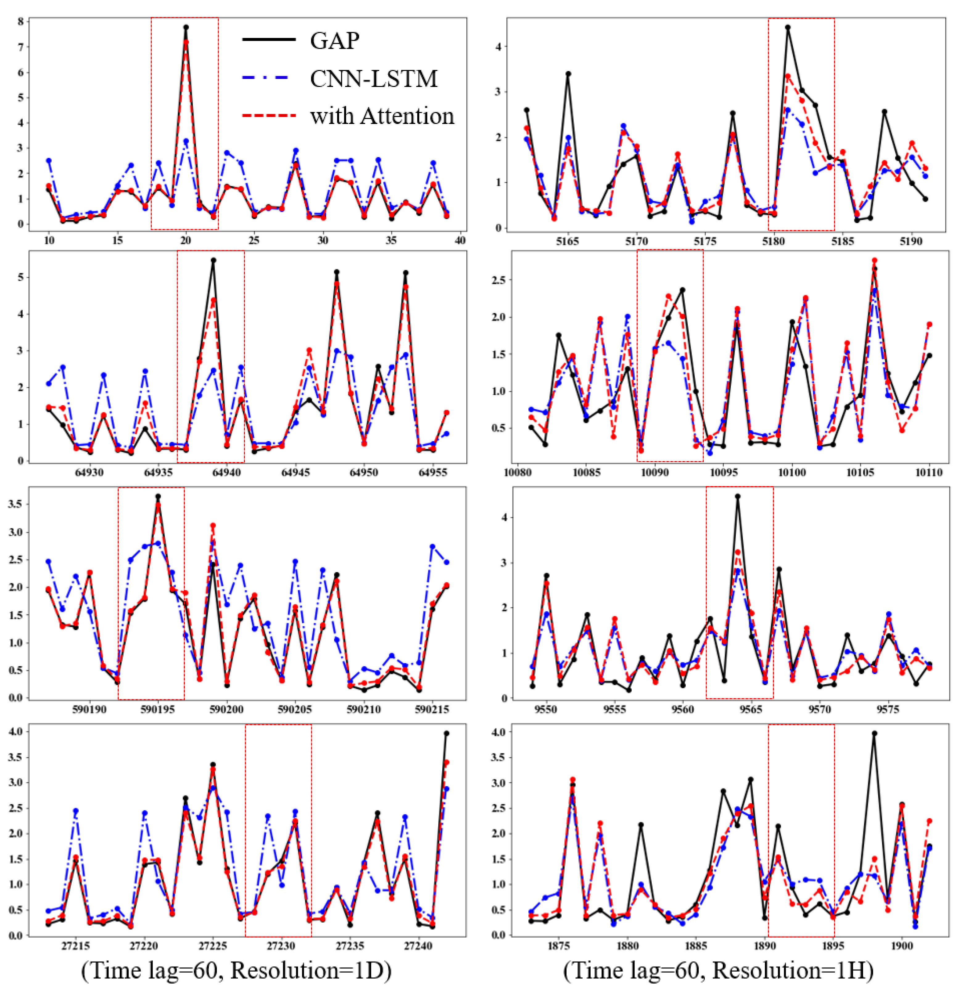
We compare the prediction performance of the proposed model with that of a competitive CNN-LSTM model by plotting the ground-truth and prediction values in Figure 8. The prediction values in the red line are quite similar to the actual power consumption values in the black line, which shows the superiority of the prediction in the transient and impulsive cases mentioned in Section 1.

4.4. Discussion

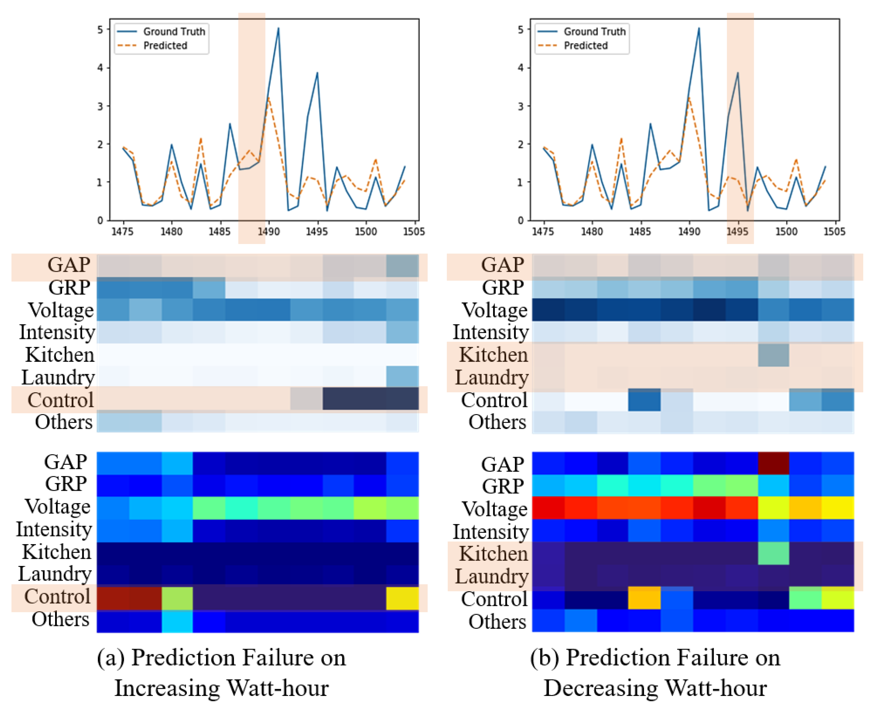
Meanwhile, we discover the two patterns of prediction failure mainly occurred in the case of Figure 9. The attention vector is uniformly distributed over all entire time steps in the window. Considering that the attention score is expressed as a probability distribution at the scale of (0,1) by the softmax operation, we conclude that the output of the deep learning models diverges and fails to extract spatiotemporal features.
Figure 9a shows the heat map of the convolutional filter for the two prediction failures that can be analyzed as the delay in weighting the control facility occurred in preparation for the sudden increase of the GAP. In Figure 9b, on the other hand, a sudden decrease in GAP without reason is observed, and it can be confirmed that it is difficult to model only by the historical power consumption data.
Taken together, in terms of the power prediction performance and the effect of the attention mechanism, we have evaluated the performance and the robustness in the transient and impulsive signals by quantitative and qualitative experiments. The general power prediction, however, still requires additional mechanism to cope with the aleatoric uncertainty [47] caused by the distribution of the power consumption data. This problem can be handled by extending the proposed model with generative deep learning and adopting the unsupervised learning.

5. Concluding Remarks

In this paper, we have proposed a deep learning model with the multi-headed attention for predicting power consumption. After addressing the issues to model the power consumption and reviewing the power prediction models based on deep learning, we have presented the proposed model of CNN-LSTM for extracting the spatiotemporal features and the multi-headed attention for learnable weighting. The model has been evaluated in various temporal conditions and the deep learning parameters are analyzed by class activation map to understand the prediction failures.
Meanwhile, events that are outside the long-term behavior can be considered as possible events happening and failure to correctly predicting them within accuracy, which the rest of the prediction profiles present, can be attributed as outlier points. As a future work, we will take care of this issue through aggregation practices which smooth out the effect of such mis-prediction, and treat it within the tolerable error by the provided flexibilities of the hybrid approach.

Author Contributions

Conceptualization, S.-B.C.; Formal analysis, S.-J.B.; Funding acquisition, S.-B.C.; Investigation, S.-J.B.; Methodology, S.-J.B. and S.-B.C.; Supervision, S.-B.C.; Visualization, S.-J.B.; Writing—review & editing, S.-B.C. All authors have read and agreed to the published version of the manuscript.

Funding

This work was partly supported by the Institute of Information and Communications Technology Planning and Evaluation (IITP) grant funded by the Korean government (MSIT) (No. 2020-0-01361, Artificial Intelligence Graduate School Program (Yonsei University)) and the Korea Electric Power Corporation (Grant number: R18XA05).

Conflicts of Interest

The authors declare no conflict of interest.

References

  1. IEA. World Energy Outlook 2019; IEA: Paris, France, 2019; Available online: http://www.iea.org/reports/world-energy-outlook-2019 (accessed on 13 November 2019).
  2. Nejat, P.; Jomehzadeh, F.; Taheri, M.M.; Gohari, M.; Majid, M.Z.A. A global review of energy consumption, CO2 emissions and policy in the residential sector (with an overview of the top ten CO2 emitting countries). Renew. Sustain. Energy Rev. 2015, 43, 843–862. [Google Scholar] [CrossRef]
  3. Zhao, G.; Liu, Z.; He, Y.; Cao, H.; Guo, Y.B. Energy consumption in machining: Classification, prediction, and reduction strategy. Energy 2017, 133, 142–157. [Google Scholar] [CrossRef]
  4. Deb, C.; Zhang, F.; Yang, J.; Lee, S.E.; Shah, K.W. A review on time series forecasting techniques for building energy consumption. Renew. Sustain. Energy Rev. 2017, 74, 902–924. [Google Scholar] [CrossRef]
  5. Arghira, N.; Hawarah, L.; Ploix, S.; Jacomino, M. Prediction of appliances energy use in smart homes. Energy 2012, 48, 128–134. [Google Scholar] [CrossRef]
  6. Prashar, A. Adopting PDCA (Plan-Do-Check-Act) cycle for energy optimization in energy-intensive SMEs. J. Clean. Prod. 2017, 145, 277–293. [Google Scholar] [CrossRef]
  7. Makridakis, S.; Spiliotis, E.; Assimakopoulos, V. Statistical and Machine Learning forecasting methods: Concerns and ways forward. PLoS ONE 2018, 13, e0194889. [Google Scholar] [CrossRef] [Green Version]
  8. Gonzalez-Briones, A.; Hernandez, G.; Corchado, J.M.; Omatu, S.; Mohamad, M.S. Machine Learning Models for Electricity Consumption Forecasting: A Review. In Proceedings of the 2019 2nd International Conference on Computer Applications & Information Security, Riyadh, Saudi Arabia, 19–21 March 2019; pp. 1–6. [Google Scholar]
  9. Burgio, A.; Menniti, D.; Sorrentino, N.; Pinnarelli, A.; Leonowicz, Z. Influence and Impact of Data Averaging and Temporal Resolution on the Assessment of Energetic, Economic and Technical Issues of Hybrid Photovoltaic-Battery Systems. Energies 2020, 13, 354. [Google Scholar] [CrossRef] [Green Version]
  10. Kim, T.-Y.; Cho, S.-B. Predicting residential energy consumption using CNN-LSTM neural networks. Energy 2019, 182, 72–81. [Google Scholar] [CrossRef]
  11. Lago, J.; De Ridder, F.; De Schutter, B. Forecasting spot electricity prices: Deep learning approaches and empirical comparison of traditional algorithms. Appl. Energy 2018, 221, 386–405. [Google Scholar] [CrossRef]
  12. Fan, H.; MacGill, I.; Sproul, A. Statistical analysis of driving factors of residential energy demand in the greater Sydney region, Australia. Energy Build. 2015, 105, 9–25. [Google Scholar] [CrossRef]
  13. Vaswani, A.; Shazeer, N.; Parmar, N.; Uszkoreit, J.; Jones, L.; Gomez, A.N.; Polosukhin, I. Attention is all you need. In Proceedings of the Advances in Neural Information Processing Systems, Long Beach, CA, USA, 4–9 December 2017; pp. 5998–6008. [Google Scholar]
  14. Zheng, H.; Fu, J.; Mei, T.; Luo, J. Learning Multi-attention Convolutional Neural Network for Fine-Grained Image Recognition. In Proceedings of the 2017 IEEE International Conference on Computer Vision, Venice, Italy, 22–29 October 2017; pp. 5219–5227. [Google Scholar]
  15. Ray, A. Symbolic dynamic analysis of complex systems for anomaly detection. Signal Process. 2004, 84, 1115–1130. [Google Scholar] [CrossRef]
  16. Rajagopalan, V.; Ray, A. Symbolic time series analysis via wavelet-based partitioning. Signal Process. 2006, 86, 3309–3320. [Google Scholar] [CrossRef] [Green Version]
  17. Lin, J.; Khade, R.; Li, Y. Rotation-invariant similarity in time series using bag-of-patterns representation. J. Intell. Inf. Syst. 2012, 39, 287–315. [Google Scholar] [CrossRef] [Green Version]
  18. Tso, G.K.; Yau, K.K.; Tso, G.; Yau, K.K.W. Predicting electricity energy consumption: A comparison of regression analysis, decision tree and neural networks. Energy 2007, 32, 1761–1768. [Google Scholar] [CrossRef]
  19. Ekonomou, L. Greek long-term energy consumption prediction using artificial neural networks. Energy 2010, 35, 512–517. [Google Scholar] [CrossRef] [Green Version]
  20. Li, W.; Yang, X.; Li, H.; Su, L. Hybrid Forecasting Approach Based on GRNN Neural Network and SVR Machine for Electricity Demand Forecasting. Energies 2017, 10, 44. [Google Scholar] [CrossRef]
  21. Mocanu, E.; Nguyen, P.H.; Gibescu, M.; Kling, W.L. Deep learning for estimating building energy consumption. Sustain. Energy Grids Netw. 2016, 6, 91–99. [Google Scholar] [CrossRef]
  22. Marino, D.L.; Amarasinghe, K.; Manic, M. Building energy load forecasting using Deep Neural Networks. In Proceedings of the IECON 2016—42nd Annual Conference of the IEEE Industrial Electronics Society, Florence, Italy, 23–26 October 2016; pp. 7046–7051. [Google Scholar]
  23. Kong, W.; Dong, Z.Y.; Jia, Y.; Hill, D.; Xu, Y.; Zhang, Y. Short-Term Residential Load Forecasting Based on LSTM Recurrent Neural Network. IEEE Trans. Smart Grid 2017, 10, 841–851. [Google Scholar] [CrossRef]
  24. Li, C.; Ding, Z.; Zhao, D.; Yi, J.; Zhang, G. Building Energy Consumption Prediction: An Extreme Deep Learning Approach. Energies 2017, 10, 1525. [Google Scholar] [CrossRef]
  25. Rahman, A.; Srikumar, V.; Smith, A.D. Predicting electricity consumption for commercial and residential buildings using deep recurrent neural networks. Appl. Energy 2018, 212, 372–385. [Google Scholar] [CrossRef]
  26. Shah, I.; Iftikhar, H.; Ali, S.; Wang, D. Short-Term Electricity Demand Forecasting Using Components Estimation Technique. Energies 2019, 12, 2532. [Google Scholar] [CrossRef] [Green Version]
  27. Fan, C.; Wang, J.; Gang, W.; Li, S. Assessment of deep recurrent neural network-based strategies for short-term building energy predictions. Appl. Energy 2019, 236, 700–710. [Google Scholar] [CrossRef]
  28. Wang, Y.; Gan, D.; Sun, M.; Zhang, N.; Lu, Z.-X.; Kang, C. Probabilistic individual load forecasting using pinball loss guided LSTM. Appl. Energy 2019, 235, 10–20. [Google Scholar] [CrossRef] [Green Version]
  29. Kim, T.-Y.; Cho, S.-B. Particle Swarm Optimization-based CNN-LSTM Networks for Forecasting Energy Consumption. In Proceedings of the 2019 IEEE Congress on Evolutionary Computation, Wellington, New Zealand, 10–13 June 2019; pp. 1510–1516. [Google Scholar]
  30. Shi, H.; Xu, M.; Li, R. Deep Learning for Household Load Forecasting—A Novel Pooling Deep RNN. IEEE Trans. Smart Grid 2017, 9, 5271–5280. [Google Scholar] [CrossRef]
  31. Bouktif, S.; Fiaz, A.; Ouni, A.; Serhani, M.A. Optimal Deep Learning LSTM Model for Electric Load Forecasting using Feature Selection and Genetic Algorithm: Comparison with Machine Learning Approaches. Energies 2018, 11, 1636. [Google Scholar] [CrossRef] [Green Version]
  32. Guo, Z.; Zhou, K.; Zhang, X.; Yang, S. A deep learning model for short-term power load and probability density forecasting. Energy 2018, 160, 1186–1200. [Google Scholar] [CrossRef]
  33. Fan, C.; Sun, Y.; Zhao, Y.; Song, M.; Wang, J. Deep learning-based feature engineering methods for improved building energy prediction. Appl. Energy 2019, 240, 35–45. [Google Scholar] [CrossRef]
  34. Hinton, G.E. Deep belief networks. Scholarpedia 2009, 4, 5947. [Google Scholar] [CrossRef]
  35. Taieb, S.B. Machine Learning Strategies for Multi-Step ahead Time Series Forecasting; Universit Libre de Bruxelles: Bruxelles, Belgium, 2014; pp. 75–86. [Google Scholar]
  36. Wang, K.; Qi, X.; Liu, H. Photovoltaic power forecasting based LSTM-Convolutional Network. Energy 2019, 189, 116225. [Google Scholar] [CrossRef]
  37. Bu, S.-J.; Cho, S.-B. A convolutional neural-based learning classifier system for detecting database intrusion via insider attack. Inf. Sci. 2020, 512, 123–136. [Google Scholar] [CrossRef]
  38. Qing, X.; Niu, Y. Hourly day-ahead solar irradiance prediction using weather forecasts by LSTM. Energy 2018, 148, 461–468. [Google Scholar] [CrossRef]
  39. Chorowski, J.; Bahdanau, D.; Serdyuk, D.; Cho, K.; Bengio, Y. Attention-Based Models for Speech Recognition. In Proceedings of the Advances in Neural Information Processing Systems, Montreal, QC, Canada, 7–12 December 2015; pp. 577–585. [Google Scholar]
  40. Zhou, B.; Khosla, A.; Lapedriza, A.; Oliva, A.; Torralba, A. Learning Deep Features for Discriminative Localization. In Proceedings of the 2016 IEEE Conference on Computer Vision and Pattern Recognition, Las Vegas, NV, USA, 27–30 June 2016; pp. 2921–2929. [Google Scholar]
  41. Kim, J.-Y.; Cho, S.-B. Electric Energy Consumption Prediction by Deep Learning with State Explainable Autoencoder. Energies 2019, 12, 739. [Google Scholar] [CrossRef] [Green Version]
  42. Sainath, T.N.; Mohamed, A.R.; Kingsbury, B.; Ramabhadran, B. Deep convolutional nueral networks for LVCSR. In Proceedings of the 2013 IEEE International Conference on Acoustics, Speech and Signal Processing, Vancouver, BC, Canada, 26–31 May 2013; pp. 8614–8618. [Google Scholar]
  43. Ronao, C.A.; Cho, S.-B. Human activity recognition with smartphone sensors using deep learning neural networks. Expert Syst. Appl. 2016, 59, 235–244. [Google Scholar] [CrossRef]
  44. Shen, T.; Zhou, T.; Long, G.; Pan, J.J.S.; Zhang, C. DiSAN: Directional self-attention network for RNN/CNN-free language understanding. In Proceedings of the Thirty-Second AAAI Conference on Artifial Intelligence, New Orleans, LA, USA, 2–7 February 2018; pp. 5446–5455. [Google Scholar]
  45. Miyazaki, K.; Komatsu, T.; Hayashi, T.; Watanabe, S.; Toda, T.; Takeda, K. Weakly-Supervised Sound Event Detection with Self-Attention. In Proceedings of the ICASSP 2020 IEEE International Conference on Acoustics, Speech and Signal Processing, Barcelona, Spain, 4–8 May 2020; pp. 66–70. [Google Scholar]
  46. Bache, K.; Lichman, M. Individual Household Electric Power Consumption Dataset; University of California, School of Information and Computer Science: Irvine, CA, USA, 2013; Volume 206. [Google Scholar]
  47. Gal, Y.; Ghahramani, Z. Dropout as a bayesian approximation: Representing model uncertainty in deep learning. In Proceedings of the International Conference on Machine Learning, New York City, NY, USA, 19–24 June 2016; pp. 1050–1059. [Google Scholar]
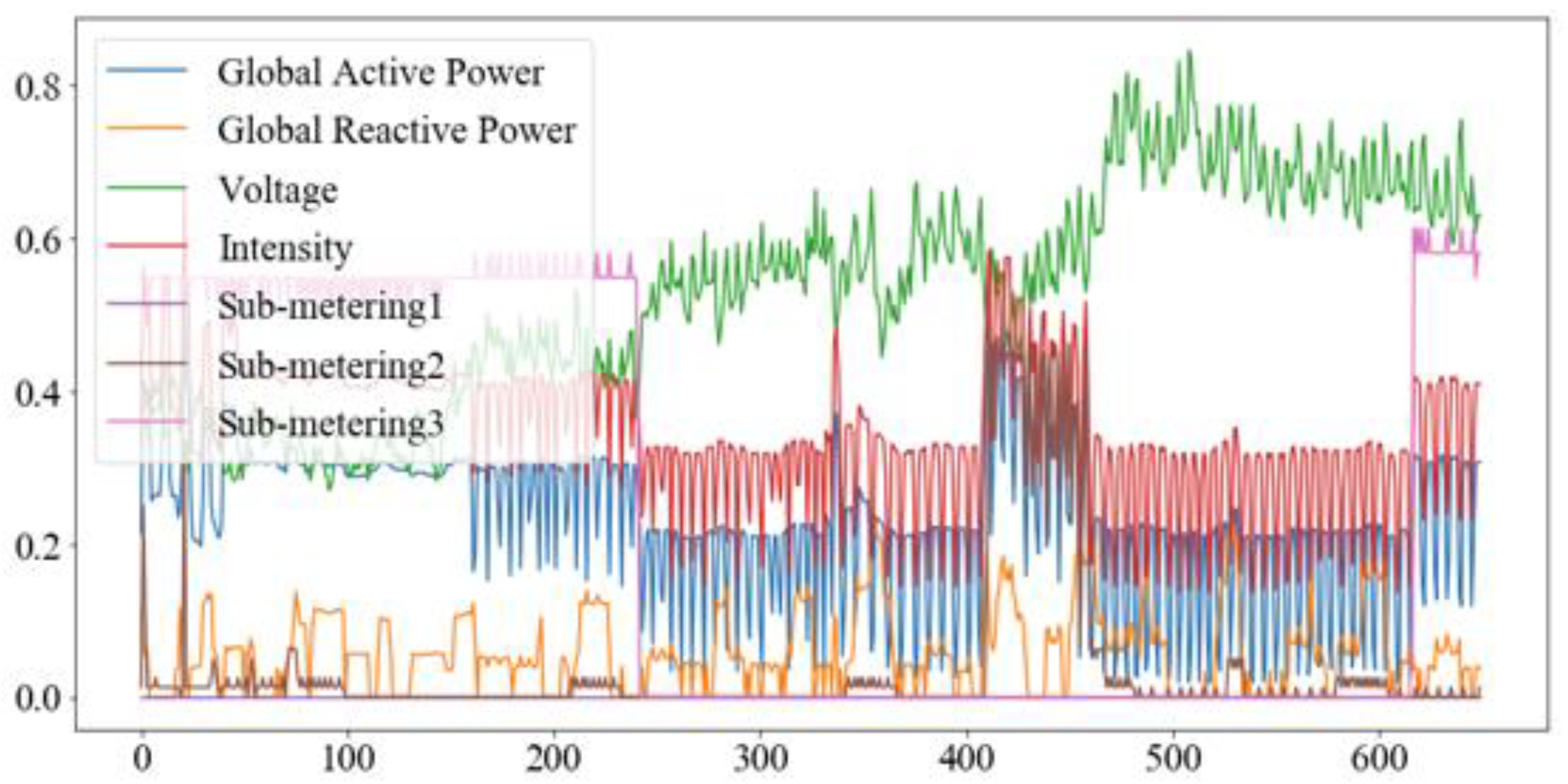
Figure 1. A typical problem formulation and the hyperparameters of the energy consumption prediction task with the resolution of the time and the time lag parameter.
Energies 13 04722 g001
Figure 2. Results of multivariate correlation of the energy attributes by the consumption level.
Energies 13 04722 g002
Figure 3. Overall structure of the proposed CNN-LSTM with multi-headed attention.
Energies 13 04722 g003
Figure 4. The operations of the multi-headed attention.
Energies 13 04722 g004
Figure 5. Implementation of the proposed CNN-LSTM with multi-headed attention.
Energies 13 04722 g005
Figure 6. 10-fold cross validation of the methods including the deep learning models.
Energies 13 04722 g006
Figure 7. Comparison of MSEs by the time lag parameter ω
Energies 13 04722 g007
Figure 8. Verification of robustness to transient, impulsive characteristics of power consumption data.
Energies 13 04722 g008
Figure 9. The gradients in the convolutional layers depicted by class activation map.
Energies 13 04722 g009
Table 1. Related works on the residential energy consumption prediction based on deep learning.
Time-ScaleAuthorDomain/DataForecasting MethodPrediction MSE
(Time-Scale)
Short
(30-min
or
1-h)
Mocanu [21]UCI Household PowerFactored Conditional Restrict Boltzmann Machine0.6211
(1-h)
Marino [22]UCI Household PowerSequence-to-sequence LSTM0.6420
(1-h)
Li [20]New South Wales and Victorian AustraliaRNN-SVR Ensemble0.4059
(1-h)
Kong [23]Smart Grid Smart City (SGSC) AustraliaRNN, LSTM0.2903
(1-h)
Li [24]Applied Building EnergyStacked Autoencoder, Extreme Learning Machine40.6747
(30-min)
Makridakis [7]M3-competition
Time-series Data
ARIMA, NN, GP, k-NN, SVR0.3252
(1-h)
Rahman [25]Salt Lake City Public Safety BuildingLSTM0.2903
(1-h)
Gonzalez-Briones [8]Shoe Store Power Data
Spain
LR, DT, RF, k-NN, SVR0.4234
(1-h)
Shah [26]Nord Pool Electricity DataSpline Function-based, Polynomial Regression, ARIMA0.2428
(1-h)
Fan [27]Hong Kong Educational Building Operational DataNN, RNN, LSTM118.2
(24-h)
Kim [10]UCI Household PowerCNN-LSTM0.2803
(1-h)
Wang [28]Irish Customer Behavior Trials, Low Carbon LondonQuantile Loss-guided LSTM0.1552
(1-h)
Kim [29]UCI Household PowerCNN-LSTM with Particle Swarm Optimization-based Architecture Optimization0.3258
(30-min)
Medium
(1-month)
Shi [30]Smart Metering Electricity Customer Behavior Trial (CBT)Pooling-based RNN0.4505
(1-month)
Bouktif [31]French National Energy ConsumptionLSTM with Genetic Algorithm-based Time Lag Optimization270.4
(1-month)
Long
(1-year)
Guo [32]China Jiangsu Province PowerLSTM, Quantile Regression594.8
(1-year)
Table 2. The attributes and statistics of the UCI household electric power consumption dataset.
AttributesDateGlobal Active Power (kW)Global Reactive Power (kW)Voltage (V)Global Intensity (A)Kitchen (Wh)Laundry (Wh)Climate Controls (Wh)
Average-1.09160.1237240.83994.62781.12191.29856.4584
Std. Dev.-1.05730.11273.24004.44446.15305.82208.4372
Max26/11/201011.12201.3900254.150048.400088.000080.000031.0000
Min16/12/20060.07600.0000223.20000.20000.00000.00000.0000
Table 3. Summary of the hyperparameters of the proposed model.
OperationNo. of Convolution Filters/NodesKernel SizeStrideActivation FunctionNo. of Parameters
TimeDistributed(Conv1D)642 × 11tanh192
TimeDistributed(MaxPool1D)- 2tanh0
TimeDistributed(Multi-Attention)- -softmax0
TimeDistributed(Conv1D)642 × 11tanh8256
TimeDistributed(MaxPool1D)- 2tanh0
TimeDistributed(Multi-Attention)- -softmax0
Dropout0.5---0
LSTM64--tanh73,984
LSTM64--tanh33,024
Dropout0.5---0
Dense64 tanh4160
Dense64 tanh4160
Dense1 linear65
Table 4. Comparison of MSE according to time resolution and modeling method (LR: linear regression; ARIMA: autoregressive integrated moving average; DT: decision tree; RF: random forest; SVR: support vector regression; MLP: multilayered perceptron; CNN: convolution neural network; and LSTM: long short-term memory).
ResolutionLRARIMA [7]DTRFSVR [8]MLPCNNLSTMCNN-LSTM [10]Ours
1M0.08440.08380.10260.08020.07970.10030.06660.07410.06600.0516
15M0.25150.24280.42340.39720.32280.23700.21230.22080.20850.1838
30M0.30500.29920.51990.39510.36190.28130.26840.27730.25920.2366
45M0.33210.34310.48040.43150.42470.32080.31830.32200.31330.2838
1H0.33980.32520.52590.43440.40590.30720.28650.29030.28030.2662
1D0.10830.09800.18910.11900.13110.11340.10690.11290.10130.0969
1W0.06240.06160.07060.06170.06200.04410.03330.03870.03280.0305
Table 5. Effect of various attention mechanisms on different neural network architectures (MSE).
Attention TypeCNN (1D)CNN (2D)LSTMCNN-LSTM
None0.07240.06660.07410.0676
Single-attention0.07010.05420.07060.0660
Multi-headed Attention0.06880.05380.06830.0516