Abstract
Society’s concerns with electricity consumption have motivated researchers to improve on the way that energy consumption management is done. The reduction of energy consumption and the optimization of energy management are, therefore, two major aspects to be considered. Additionally, load forecast provides relevant information with the support of historical data allowing an enhanced energy management, allowing energy costs reduction. In this paper, the proposed consumption forecast methodology uses an Artificial Neural Network (ANN) and incremental learning to increase the forecast accuracy. The ANN is retrained daily, providing an updated forecasting model. The case study uses 16 months of data, split in 5-min periods, from a real industrial facility. The advantages of using the proposed method are illustrated with the numerical results.
1. Introduction
The definition of pricing schemes and investment strategies in the electric sector can be affected by the uncertainty in the consumption, generation, and generation costs [1,2]. Smart grids can improve the management of electricity by providing the means to supply relevant data to support decisions [3]. The reduction of energy cost and energy life extent are two important points studied in the context of smart grids [4]. These aspects are within the context of Demand Response (DR), which is related to the reduction of electricity consumption in particular periods in order to decrease the electricity costs [5,6].
The forecasting tasks raise answers in smart grid environments and within the DR context in the domain of power system operation and planning [7]. The demand response also has a big impact on the power system, easing the balance between the production and the generation [8]. Moreover, smart grids enable access to large volumes of data that can have a great impact on the monitoring of these power systems [9].
The energy management of a building’s real-time measuring data may be used in energy forecast tasks in a building in order to optimize the management of energy [10]. An Artificial Neural Network (ANN) trained with optimization algorithms is a model composed by neurons structured in layers and linked through weighted connections. The layers include the input layer that receives the data, the output layer that provides the result, and the hidden layers that perform the operation between the input and output with the support of activation functions. Moreover, ANN is described by an iterate process that uses the feedforward algorithm in order to calculate the output, but also uses the backpropagation algorithm in order to improve the network itself. This is a process repeated for a consecutive amount of times [11,12]. K-Nearest Neighbors (KNN) is a non-parametric learning algorithm that makes forecasts by calculating similarities between input samples and training instances. This is accomplished with the distance metric support, which identifies the nearest neighbors [13,14]. RF is an ensemble algorithm that supports the creation of multiple decision trees with random possibilities, each one capable of producing a response. The prediction will be composed by the response with the highest votes [15].
The algorithm can be used in a varied number of applications. Electricity price forecasting is one of these examples that has received accurate results for hour-ahead applications [16]. Wind energy applications can also be taken as an example, showing that with different network structures and different parametrizations, the results of ANN are different [17]. Additionally, long term applications are also considered, such as the forecasting of electrical power demand [18]. The use of univariate and multivariate methods in industrial load consumption contexts is discussed [19].
In the present paper, the major novelty aspect is the implementation of an incremental learning approach, which benefits from the most recent consumption values available to train the ANN incrementally, supported by adequate data pre-processing for the electricity consumption in an industrial building. The proposed methodology uses real-time data and forecasting algorithms in order to improve the forecasts of industrial facility electricity consumption. The research and application of electricity management solutions integrated in the context of industrial facilities and demand response scenarios was addressed by the authors of the present paper in [20]. The use of five-minute periods for forecast tasks as well as the inclusion of a one-week test and more than one-week train sets are considered in [20]. However, while in [20] the forecasting technique that provided more accurate results in a specific building based on different input decision scenarios was selected with the support of trial and error processes, in the present paper incremental learning is used in order to re-train the implemented ANN. In this way, it is proposed to run the training service regularly in order to capture the most updated behavior of electricity consumption. An ANN is used [21], as it was found in previous research to be the most adequate forecasting technique in this application. Additionally, the goal of this paper is to research the best forecasting technique model option and to use incremental learning in order to keep track of updated information, thus improving the forecast results. The first stage of the proposed methodology describes how to deal with missing and incorrect data. In the second stage, the forecasting service is supported by periods split by 5 min intervals. Every day at midnight, the training data is updated during the forecast process.
After this introduction, the time series forecasting is explained with detail with the support of forecasting applications in Section 2. The different stages of the proposed methodology are explained in Section 3. In Section 4, a case study explores the aspects considered in the study. The results of the case study are shown with detail in Section 5. Finally, Section 6 presents the main conclusions.
2. Time Series Forecasting
Load forecast applications studied within the scope of industrial facilities keeps an open view about particular factors useful in the industrial domain [22]. In fact, load forecast is very relevant for example in the scope of the DR, which brings technical and economic potential to industrial energy facilities [23]. Strategies to deal with demand response problems are discussed, in order to balance the demand for the power with the supply and to reduce the energy in peak load periods, in [24,25]. The load forecast is, in fact, a time series forecast. Recent literature has shown that time series forecasting is a field integrated in the machine learning domain with focused research in many publications [26]. In fact, a lot of these publications explore neural networks applications recognizing the importance of the algorithm architecture decisions [27]. Time series forecasting is a process that predicts future events based on a historical trend with data that has an active role in business decision making in several domains. Moreover, researchers take into account traditional time series techniques such as ARIMA and SARIMA, while also considering advanced techniques including BATS and TBATS [28]. The time series forecasting is stated to be fundamental for many applications, including business, stock market, and exchange. Additionally, several researches study the different forecasting algorithms in their performance including Artificial Neural Networks (ANN), Support Vector Machine (SVM), genetic algorithms, and fuzzy time series methods [29]. As mentioned in [27], some time series forecasting problems study architectural decisions of ANN models instead of researching the performance of several forecasting algorithms. The research in [30] proposed a new model considering a systematic procedure in the model’s construct. Recurrent Neural Networks are stated as powerful tools in solving various models [31]. Multivariate time series predictions are used on several time series fields, including power energy, meteorology, finance, and transportation [32].
The existence of large amounts of historical data and the need to obtain accurate forecasts leads some researches to study machine learning strategies to deal with time series problems [33]. Moreover, some researchers provide importance to classical methods providing capabilities that include problem solving, storing memory, and understanding human language [34]. In fact, problems concerning energy-related data for time series forecasting, more specifically electrical, solar, and wind energy problems, have a great impact on society [35].
The complexity of the time series is a topic explored in [36]. In fact, smart building monitored data is a recommended complexity time series example, giving importance to sensor data measuring several devices that should provide more complete information, including heating and air conditioning data [37]. The research taken place states that data mining applications outperforms the classical ones. Error evaluation metrics are a crucial point in the algorithm’s evaluation used to prove this aspect [38].
3. Methodology Description
In this section, the proposed methodology is described step by step. These are split in parametrization and dataset reducer, training service, forecasting service, and forecast accuracy analyzer. The set of steps is integrated in several machine learning tasks, which include the extraction and reduce of data, the analysis of the best algorithm application, the cleaning of data, and the scheduled forecasts. Considering the existing real-time data, a sample representing consumption data is sent initially to trigger activities known as the dataset reducer and the forecasting parametrization decision maker that intends, respectively, to perform data selections and parametrization decisions with the goal of providing more accurate forecasts. The resulted data from these two activities are sent to the training service where the data cleaning activity intends to perform operations resulting in more reliable data. Still, in the training service, the training activity makes data adjustable and prepared for forecasting tasks. The forecasting service uses the prepared data to perform the intended forecasting tasks with the Artificial Neural Networks (ANN) algorithm. The proposed methodology diagram is presented in Figure 1.
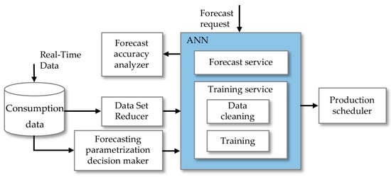
Figure 1.
Proposed methodology diagram regarding the forecast and production planning update. ANN: Artificial Neural Network.
3.1. Parametrization and Dataset Reducer
The first step, which includes parametrization and a dataset reducer, focuses on the parametrization of parameters integrated in the data warehouse domain. The actions involved in this step are focused on two aspects that intend to provide more accurate forecast results. Both aspects require the analysis of a sample with consumption data featuring similar behaviors as the real-time data. The real-time data is the monitored energy from an industrial facility. The first aspect, known as the data set reducer, considers the simplification of data to a new version with a similar content to the original version but with fewer details. The exclusion of irrelevant and unwanted information is a task of big importance that has impact on the forecasting reliability. However, discarding information might mean that relevant information is being discarded as well. Hence, there is a balance between proving complete information and avoiding the excess of data. The dataset reducer performs automatic operations selecting subsets of data, gathering the most recent and relevant information. Thus, the reduction of data is intended to be activated each day at midnight, gathering more updated information, while discarding older content in order to keep the same dimension of data. More precisely, each time the data reduction is triggered, the information is updated, with the data belonging to the next day of the week while the data corresponding to the older day of the week is discarded.
Although the reduced version is applied to the historical data, the same insights apply to the real-time data. The second aspect known as forecasting parametrization decision maker considers the definition of parameters that should provide more reliable forecasts. The first parameter, known as the learning rate, consists of how precise the algorithm should learn with the provided data. Smaller rates result in a more precise analysis with the disadvantage of taking more time, while larger rates on the other hand perform less accurate analysis providing the results for lower periods of time. The learning rate should be a small rate, taking into account that it should not be lower than needed in order to provide the learned analysis in a reasonable time. The hidden layers neurons consist on how much neurons should support the hidden layers. The number of neurons should be big enough to a more supportive learning process resulting in more accurate forecasts. The number of epochs consists of the quantity of iterations that the model is trained. Larger numbers of epochs correspond to additional training, while overfitting can occur if the number of epochs is too large. An early stopping parameter is used to overcome the overfitting issue, allowing to stop training the model when no further improvements are being made. Using early stopping enables using a larger number of epochs while preventing overfitting. The validation split consists of the percentage of data that should be considered in order to validate the data.
Both the reduced version of the dataset and the machine learning architecture are sent, respectively, from the dataset reducer and the forecasting parametrization decision maker to the training service. This step is only run once.
3.2. Training Service
The training service is a step that performs training tasks in the context of the machine learning domain. The activities implicit in this service are split in two tasks, the data cleaning and the training with data. Moreover, the mentioned tasks are influenced by the Artificial Neural Network (ANN) method, which is reliable on the most recently updated data available in order to achieve more accurate forecasts. The data cleaning reorganizes the data sample, making it suitable for forecast operations. Additionally, it performs data manipulation operations that intend to make it more understandable by the forecasting technique. It is noted that measured and recorded data might be very inconsistent, overloaded, and confusing. Therefore, the sampled data are rearranged through cleaning data operations in a varied number of ways in order to produce more accurate information. The first aspect considers the gathering of data, which reads the consumption and the time it was recorded and places that information in six different fields: year, month, day, hour, minutes, and consumption by kWh. Afterwards, the adjustment of time reads the minutes information exactly in which instance it was recorded and replaces it instead by the time period that the instance belongs to. This is accomplished by if-then rules. The information associated with the six different fields is saved, keeping the system aware of the information of that period during the next gathering of data. This strategy makes it possible to observe a subset of data and make decisions where it is necessary to manipulate it to make sure that each time period is unique and associated to a single consumption, thus providing complete information but avoiding overloaded data at the same time. The detection of missing data is accomplished with if-then rules and triggered if the time period that is supposed to succeed the previous measurement does not match the actual time period, meaning that there are time period measures that were not monitored and recorded. The addition of missing information is accomplished by adding duplicated consumptions belonging to the previous time period until there are no more consumptions to be added which eventually breaks the loop. Furthermore, the aggregation takes an active role by summing consumptions that belong to the same time period, thus making sure that a time period has a unique consumption. The strategy consists of keeping summing the consumptions from each iteration until it detects that a new iteration takes place in the actual time period, which leads to save the aggregated consumption in the set of inputs. Finally, the outlier treatment is also applied by removing any outliers existing in the dataset and replacing it by the mean of the occurrence that is presented previously and afterwards. The outlier’s detection is accomplished by the average and standard deviation calculations and if-then conditions. The mentioned statistics calculations are represented, respectively, in Equations (1) and (2):
where A is the average industrial energy in F, n is the current moment, E is the industrial energy, t is the exact period, and F is the frame as basis for A calculation.
where S is the standard deviation industrial energy in F, F is the frame as basis for SD calculation, n is the current moment, t is the exact period, E is the industrial energy, and A is the average industrial energy in F.
The average and standard deviation calculations are obtained as evidenced in Equations (1) and (2) with the gathering of industrial energy information placed on periods between the current moment and a frame created as basis. More concretely, the frame represents the time period that the user is distanced from the current moment. The average frame is described by the ratio between the sum of a sequence of industrial energy values placed in an exact period by the established frame. The standard deviation represents the squared root of the inverse frame times the sum of the difference between the average and the respective current moment industrial consumption placed on a time period.
The outliers’ existence is detected with the support of if-then that considers that outlier anomalies are featured under one of the two possible conditions. The first anomaly case states that the value obtained is higher or equal than the sum of the average and a multiple version of the standard deviation across an established frame. Alternatively, a second anomaly case states that the forecast value obtained is lower or equal than the difference of the average and a multiple version of the standard deviation across an established frame. The correction strategy to deal with these anomalies consists of replacing the actual values with the average of the values that precede and succeed the original counterpart. Further details concerning the detection and correction of these anomalies can be seen in Equation (3):
where A is the average industrial energy in F, ε is the error factor, E is the industrial energy, t is the exact period, S is the standard deviation industrial energy in F, F is the frame as basis for SD calculation.
The error factor represents a quantitative number that multiplied by the standard deviation provides awareness about how detailed the outlier detection is concerning the deviation of each industrial consumption to the average placed on an exact period. Therefore, larger error factors tend to assign fewer outliers.
Additional and manual cleaning operations are required in order to deal with the existence of weeks with unreliable data. The strategy consists of deleting weeks presenting this anomaly. The presence of data featured by non-useful days is considered unreliable, and as such validates the discarding of these days from the week samples. The new version of data resulted from all these cleaning operations is characterized by its greater interpretability allowing forecasting techniques to use more reliable information, which results in fewer errors. The training operations considers that the split of the data resulted from the cleaning operation in training and test data, the first one featuring the historical data and the latter featuring the forecast targets.
This step is performed automatically after the ending of the tuning process; however, it is possible to be run again with the triggering of training requests. Regardless of the event that triggers the training service, it should be noted that the running of the tuning process is a prerequisite as manipulate data operations integrated in the training service require the reduce version of the dataset obtained from the tuning process. Additionally, the machine learning technique needs to be received by the training service in order to later be used in the forecast service. The production scheduler has an active role in the training service required at certain points in time, and retrains data in order to achieve lower forecast errors on the forecast service.
3.3. Forecasting Service
The forecast service is a step that performs prediction tasks scheduling; each one of the observations is present in the set of test targets. The forecasting service receives the resulted data split on the training and test sets with the best interpretation and with a suitable structure for machine learning tasks. The predictions of the test sets are supported with the Artificial Neural Network (ANN) method and triggered inside the forecasting service with the support of a production scheduler. This scheduler determines the respective test iteration to be forecasted. The forecasting service with the information provided by the scheduler makes the predictions and additionally asks the forecast accuracy analyzer to provide its test evaluation.
This step is performed automatically after the end of the training service; however, it is iteratively run again according to the schedule, which is synced to the test targets. The schedule will determine the last iteration according to the set of test observations. Additionally, it is possible to run this step again by triggering a new forecast request, which triggers the training service in order to update the training information as a means to improve the forecasts.
3.4. Forecast Accuracy Analyzer
The errors calculations provide awareness about the deviation of the obtained values in the predictions from the actual values. These error values measure the performance of each one of the algorithms. This study applies the weighted absolute percentage error (WAPE) and the symmetric mean absolute percentage error (SMAPE). More concretely, WAPE is an error metrics that measures the ratio between the sum of absolute differences of the predicted value and the actual observation divided by the sum of the actual observations. Detailing SMAPE, this evaluation measure is an error metric provided by the ratio between the absolute difference of the predicted difference and the actual demand divided by half between the sum of the predicted value and the actual demand. Further details concerning the calculation of WAPE and SMAPE can be visualized in Equations (4) and (5):
where EF is the forecast industrial energy, F is the frame as basis for calculation, and t is the period.
The error metrics WAPE and SMAPE were classified in this problem as the most pragmatic evaluation choices concerning the problem at hand. Similar metrics to WAPE and SMAPE were researched including the mean absolute error (MAE) and the mean absolute percentage error (MAPE). MAE lacks a scale to the average demand, which generally results in low accuracy; thus, the MAE metrics ends up being discarded from this study. While MAPE, like WAPE, provides awareness about the magnitude of the errors in a set of predictions, the first one presents one problem. MAPE calculates the ratio for each iteration, placing the actual consumption instead of the sum of a set of energy values in the denominator. Therefore, there is a risk of a real consumption being null and the division being impossible. To avoid this issue, WAPE is used instead, as an alternative for MAPE. Additionally, a square metrics known as root mean square percentage error (RMSPE) was also studied. This metrics replaces the absolute difference with the square deviation of the demand and the predicted counterpart. Hence, RMSPE provides awareness about the distance of the errors in the set of predictions in addition to the magnitude already provided by WAPE. However, a disadvantage was found in RMSPE, which impacts a lot the accuracy of predictions. This metric does not treat each error the same giving more importance to the biggest errors. Therefore, a big error is enough to result in a very bad RMSPE in a set of predictions recalling the square deviation notion.
4. Case Study
The historical data of the industrial company is composed by a set of consumptions provided from five to five minutes. The selected data is set from 1 January 2018 to 13 April 2019, presenting a total of 62 weeks. The weekly consumption is visualized in Figure 2, which shows all the weeks in the data set. Additionally, the time series present in Figure 2 present a set of 1728 in the time axis, which corresponds to one week of 6 days concerning periods of 5 min.
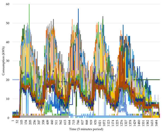
Figure 2.
Weekly consumption from 1 January 2018 to 13 April 2019. Each line is one week (1728 points).
The 62 weeks presented from 1 January 2018 to 13 April 2019 show a very similar behavior presenting five daily patterns from Monday to Friday featuring industrial consumptions behaviors that are usually in a range between 0 and 50 kWh, and a Saturday pattern featuring low activity usually below the 20 kWh. Although the case study featuring the 62 weeks provides low insights about the daily progress for each one of the six days, a few observations can be identified. The week starting featured by the Monday early morning presents consumption behaviors near the 0 kWh due to the continuation of Sunday, which presents no activity at all. The consumptions activity starts at some point during the Monday morning presenting consumptions increases that grow from nearly 0 kWh to above 20 kWh. This is followed by nonlinear variations that stay in the range between the 10 and 50 kWh. The end of the day features low consumptions staying below the 10 kWh.
The pattern is repeated, respectively, for Tuesday, Wednesday, Thursday, and Friday. The only difference is that the early mornings of each day are represented by low consumptions that stay below 10 kWh instead of the continuation of Sunday behavior, where there is no activity at all.
Saturday presents very low activity staying below the 20 kWh slowly decreasing as the day progresses until it starts reaching the Sunday beginning, which features no activity at all. Although each one of the 60 weeks present different behaviors, the daily patterns follow the mentioned behavior.
5. Results
This section presents the obtained results using the case study presented in Section 4. The covered points are synced with the aspects explored in the methodology presented in Section 3. The Section 5.1, Section 5.2, Section 5.3 and Section 5.4 cover all the observations and insights from each phase taken from the proposed methodology.
5.1. Parametrization and Dataset Reducer
This sub-section is based on the methodology illustrated in Figure 1 and explained with further detail in Section 3.1. The reduction of data is the first aspect to be studied. The historical data supports a fixed size of 61 weeks in any weekday forecast. Thus, retraining, featured in Section 3.2, requires the participation of the reduce process in order to discard older information while new information is updated. Moreover, the decision making concerning the parametrization of the algorithm studies the best alternative that should provide more accurate results. Two error metrics, including WAPE and SMAPE with the appliance of ANN, provide awareness about data reliability targeting 8 to 13 April 2019 (last week of April 2019 with no holidays). Moreover, six different architectural options for ANN method parametrization are considered, as presented in Table 1, focusing on changes in the learning rate and the number of neurons in intermediate layers.

Table 1.
Forecast result errors with different ANN method architectures. WAPE: weighted absolute percentage error; SMAPE: symmetric mean absolute percentage.
The presented errors show that WAPE is a more reliable option in order to measure the forecast performance. The results obtained for one-week test lead to low forecast errors staying in a range between 8.5% and 13.5%. It is noted that there is a higher number of neurons in the intermediate layers, although the forecast results need more time to be obtained, these are shown to be more accurate. Additionally, it is observed that an increase of the learning rate causes a decrease in the time processing. This is an understandable insight, as the increase of the learning rate causes a less accurate analysis, allowing to perform searches in less time. Moreover, the time processing decrease effect is less reflected with a higher amount of neurons used in intermediate layers. It is observed that a higher learning should provide more accurate forecasts only and only if a sufficient number of neurons is used in the intermediate layers.
This is demonstrated in the third and fourth execution, resulting in a higher error with a higher learning rate, which uses 32 neurons in intermediate layers, while the first and second with 64 neurons and the five and sixth with 128 neurons are shown to result in fewer errors. The architecture presenting a learning rate of 0.005 and an amount of 128 neurons in the intermediate layers, as displayed in the sixth execution, is shown to be the ANN model alternative that provides more accurate results. Although the use of a higher number of neurons results in obtaining more accurate forecasting results in more time, the time response difference compared with the other scenarios is not very reflective; thus, the accuracy of the forecasts gains the advantage. Using 128 neurons is more than enough in order to obtain more accurate results with a higher learning rate. The remaining parameters are the same for all the six methods: Clipping ratio = 5.0; EPOCHS = 500; Early stopping = 20; Validation split = 20%. The validation split was defined with a percentage of 20%, corresponding to the insights taken from several experimental tests in the present work.
5.2. Data Cleaning
The set of decisions and applications concerning data cleaning operations with regards to the methodology is illustrated in Figure 1 and explained with further detail in Section 3.2. After obtaining the results of this scenario, we focused on analyzing how the different cleaning operations influence the dataset and additionally researched the interpretable level made to the new version of data. Several processing operations are applied to raw data in order to produce more accurate information. Time adjustments are relevant procedures that guarantee the flexibility of data, transforming data placed in confusing and questionable periods to a new version of data placed on uniform and consistent periods. However, this processing operation is not enough to guarantee flexibility using weekly patterns of data, as missing information in addition to the existence of information placed on duplicated periods creates some uncertainty on the dimension of data that might be different from week to week. After solving the last issues, it is possible to achieve consistent and uniform data concerning the weeks dimension, an aspect that is very unlikely to happen in the raw version of data. Additionally, weeks with low activity present in the raw version of data lead to weekly patterns with different behaviors which are not consistent with the reliable weeks. Furthermore, Sunday’s information, present in the raw version of data and removed on the cleaned version of data, provides more empty space between the Saturday evening and the Monday morning, featuring a longer period of low activity. The outliers’ existence is also an issue that, in addition to the low reliability impact on data, provides difficulty to analyze the data set behavior. In order to understand the data impact present in all these issues, two different versions of the consumption dataset are compared: one for raw data and the other one the result of data transformations, which include the missing information handling and the removal of outliers, as can be seen in Figure 3 and Figure 4. The sub-figure highlighted in the dashed-grey line in Figure 3, left side, is a zoom in the consumption data from periods 1 to 140,181 in the right side of the figure, making it possible to see the consumption in that interval.
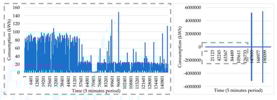
Figure 3.
Consumption raw data from 1 January 2018 to 26 September 2019.
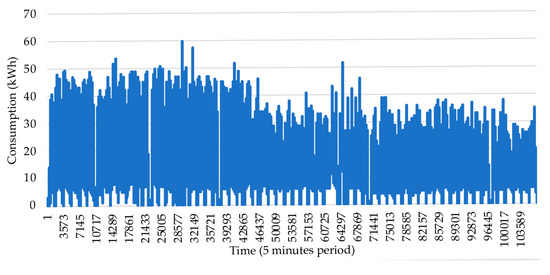
Figure 4.
Consumption cleaned data from 1 January 2018 to 13 April 2019.
The data are originally very inconsistent, presenting a lot information out of the 5-min context, leading to an uninterpretable analysis. Furthermore, the visualized outliers in the dataset are very distant from the remaining data, leading to very unrealistic scenarios. Hence, the raw data visualization provides low insights. The outlier removal clearly reduces the unrealistic consumptions allowing a more careful analysis of the consumption variability in the entire set. The time adjustment, aggregation, adding of missing records, and removal of unreliable weeks and Sundays lead to very consistent week patterns.
During the whole process, consumption tends to increase and to decrease a lot. Sequential weeks follow a very similar consumption variability. While following a similar week pattern during the entire time, it is clear that there are times with lower and higher activity. In early 2018, the consumption clearly shows a significant amount of energy consumption, namely, 50 kWh. This at some point decreased to 40 kWh. The impact of outlier removal is further researched in the test set measured from 8 to 13 April 2019. The raw and cleaned versions of data can be visualized for the period 8 to 13 April 2019, respectively, in Figure 5 top and bottom. The test data originally provide good insights about the consumption behavior during the whole time. The presence of a visible outlier in the raw version of the data reduces the interpretability of data.

Figure 5.
Consumption profile from 8 to 13 April 2019 before and after the application of the cleaning operations represented, respectively, in top curve and bottom curve.
After the cleaning treatment, which includes the outlier correction, the mentioned problem is no longer an issue, resulting in a more detailed consumption progress visualization. It is observed that the cleaning operations, which include time period corrections, the adding of missing data, and the aggregation of excess records, results in the shift effect present in the cleaned data, ultimately correcting the total time period to 1728 observations, which corresponds to the six days featuring Monday to Saturday. Consumption initially tends to stay nearly null until the early morning of Monday due to the continuity of no activity from the previous Sunday. At some point in the early morning, the device measures start registering activity; a gradual consumption that reaches an acceptable consumption of above 15 kWh in a very small period of time. The activity behavior from Monday to Friday follows a similar pattern that is described by a tendency to stay at a range from 16 to 25 kWh during the activity time and a tendency to stay above the 5 kWh and below the 16 kWh during low activity times, representing the time period between the late evening to the next early morning. There are, however, a few consumption measures during the activity times that exceed the 25 kWh, which is a breaking point out of the normal behavior. This, however, is not true for Friday, as the device measurements have little activity on Saturday during the whole day, measuring consumptions between 5 and 10 kWh, with no activity at all at the end of the week.
5.3. Training and Test Data Set
The split of the data in the training and test sets is explored using the methodology visualized in Figure 6 and explained in further detail in Section 3.2. The total dimension of data is described with a size of 62 weeks featuring the period from 1 January 2018 to 13 April 2019. This is split in 61 weeks for training featuring the period of 1 January 2018 to 6 April 2019 and one week of testing featuring the period 8 to 13 April 2019. Figure 6 shows the dimension and behavior of data detailing with more precision one training week and one test week.
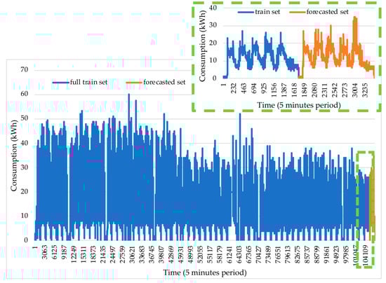
Figure 6.
Consumption monitored with a one-week test, measured from 8 to 13 April 2019, and the historical time period of the 61 weeks preceding 8 April 2019.
The consumption variability usually stays on a range between 0 and 50 kWh. There are, however, some exceptions that go above the 50 kWh and still below the 62 kWh. While the consumption behavior during the 62 weeks provides poor daily and weekly insights, it is clear that a nonlinear behavior is present that notices the activity time for sequence periods followed by low activity featuring a period out of the work schedule. This is a pattern that is repeated a lot of times, an understandable behavior considering the 62 weeks; it is logical that each of the six days in each week features activity consumptions followed by consumption behaviors that are out of schedule before the next day. A more precise study featuring the last week of training featuring the period from 1 to 6 April 2019 and the test week featuring the period from 8 to 13 April 2019 provides more precise insight for each one of the six days of the week in the weekly pattern present. The consumption data has six patterns for the train and test sets, featuring a total of 288 observations for each day and 1728 for each week.
In Figure 6, the graph on the dashed green line is the detail of the region selected in the main graph by the green dashed box. The pattern start is featured by activity below 3 kWh, followed by industrial activity that is usually between 16 and the 25 kWh, possibly with some industrial activity exceptions with behavior above 25 kWh and below 40 kWh. The usual pattern featuring 16 to 25 kWh is followed by a period of low activity between 5 and 10 kWh. This is a daily pattern, with 288 observations that is repeated five times, one for each day of the week, specifically Monday to Friday. Moreover, a different daily pattern is present for Saturday, which also featured 288 observations, where the industrial consumption stays below 15 kWh, followed by the end of the week, which keeps the consumption below 3 kWh. The redundant daily pattern from Monday to Friday with 288 observations plus the Saturday pattern with 288 observations reflects a weekly pattern of 1728 observation.
5.4. Forecast
The scheduled forecasts and the retraining process are illustrated in Figure 1 and are further explained in Section 3.3 and Section 3.4. The forecasts are scheduled to run for all five minutes instances of the weekdays concerning Monday to Saturday. The error metrics are calculated for each one of the five-minute period, giving a total of 288 periods per day, and thus, 1728 periods for the six days of the week. The retrain process is triggered in order to decrease the forecasting error. This is a decision taken every day of the week at midnight triggered for the set of weekdays: Tuesday, Wednesday, Thursday, Friday, and Saturday. Additionally, the calculated forecast on each day of the week from Sunday to Friday represents the forecasts made for the respective day and with updated information from that day for the remaining week. Thus, the Sunday forecast will predict from Monday to Saturday, while the Monday forecast will update the Monday information, hence predicting from Tuesday to Saturday. The final forecast errors for each train are calculated, as can be seen in Table 2. Moreover, the forecast of each five minutes period is illustrated in Figure 7, and the forecast errors of each five-minute period are illustrated in Figure 8. A detailed explanation of the information in Table 2 is as follows:
Table 2.
Forecast result errors for each train.
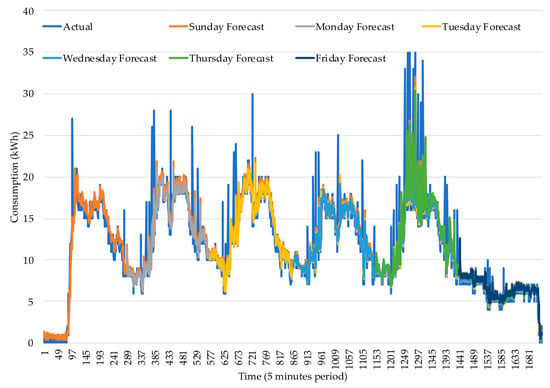
Figure 7.
Consumption forecast target for period 8 to 13 April 2019.
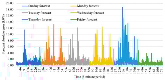
Figure 8.
Consumption forecast errors for period 8 to 13 April 2019.
- The Sunday forecast uses a historical period between 1 January 2018 and 6 April 2019 and a forecast period between 8 and 13 April 2019, described by a historical period of 61 weeks and a forecast period of one week;
- The Monday forecast uses a historical period update, discarding 1 January 2018 and adding 8 April 2019, while the forecast updates the Monday information;
- The Tuesday forecast uses a historical period update, discarding 2 January 2018 and adding 9 April 2019, while the forecast updates the Tuesday information;
- The Wednesday forecast uses a historical period update, discarding 3 January 2018 and adding 10 April 2019, while the forecast updates the Wednesday information;
- The Thursday forecast uses a historical period update, discarding 4 January 2018 and adding 11 April 2019, while the forecast updates the Thursday information;
- The Friday forecast uses a historical period update, discarding 5 January 2018 and adding 12 April 2019, while the forecast updates the Friday information.
Table 2 provides an overview of the retraining forecast improvements. The results provided by the Monday to Friday forecasts show that the improvements are reflected on Monday, Wednesday, Thursday, and Friday. Although the Thursday and Friday forecasts provide higher accurate predictions than the Sunday forecasts, accuracy improvement is only reflected for the Monday and Wednesday forecasts. The error provided for each five-minute period has a nonlinear behavior that stays in a range between the 5% and the 70%.
In fact, looking in detail at the obtained results, one can see that the proposed approach can be useful when a change is verified in the consumption process due to the update of factory commitments, for example. In such a case, knowing that the consumption context is changed, the training should be updated.
Looking at the results presented in Figure 7 and Figure 8, one can see that the absolute error provided for each five-minute period illustrated in Figure 8 is described by a sequence of nonlinear behaviors featuring a tendency to stay in a range difference between 0 and 2. This information, along with the total absolute error being 20.00 kWh, shows that there is a frequency to stay in a low error range between 0% and 10%. Some particular five-minutes periods, on the other hand, feature unreliable forecasts that do not exceed a difference higher than 19 kWh.
The Sunday forecast initially provides low errors for many sequential periods, until it reaches a sequence of five-minute periods usually in an error difference range between 2 and 6 (10 to 30%) followed by a sequential period that tends to stay in an error difference near a value 2, about 10%. The Monday forecast features frequent five-minutes periods with low absolute errors with ranges between 0 and 1 (0 to 5%); however, on the other hand, it also contains some high forecast errors that reach absolute differences between 2 and 12 (10 to 60%). The Tuesday forecasts are featured by many sequential five-minute period absolute errors in a range between 0 and 2, or, in other words, 0 to 10%. The Wednesday forecast features initial absolute differences between 0 and 1 followed by absolute differences between 0 and 2, meaning that an initial tendency to stay in a range between 0 and 10% is followed by a tendency to reach higher errors more precisely between 0 and 20%.
The Thursday forecasts have errors that are initially in a range between 0 and 1 featuring the 0 and 5% error interval, followed by many incorrect forecasts reaching error percentages above 40%, until it again resumes the absolute error difference behavior that stays in a range between 0 and 1. The Friday forecasts feature frequent absolute error differences between 0 and 1 (0 to 5%), with a few present sequential periods between 1 and 2 (5 to 10%). Although Monday presents higher forecast errors on more periods than Sunday, the latter presents lower periods that stay in a range between 0 and 1 (0 to 5%); thus, Monday generally presents better forecasts than Sunday, as evidenced in Table 2. Moreover, while the nonlinear behaviors featured by lower absolute differences on Wednesday are very similar to Sunday, the better results obtained for Wednesday leads to the insight that Wednesday presents more sequential periods with lower absolute differences. Tuesday, however, as evidenced in Table 2, leads to the insight that it presents more sequential periods near 2 (near 10%) than 0, enough to lead to a worse forecast than Monday. Thursday presents many unreliable forecasts, leading to worse forecasts than Sunday. Friday certainly presents better forecasts than Monday, featuring more sequential periods between 0 and 1 (0 to 5%).
With more detail, for the forecast made on Friday (regarding the consumption on Saturday), which is selected as an example for illustration purposes, Figure 9 presents the actual and the forecasted consumption for 13 April 2019. It can be seen that the most updated forecast, with more recent data that is adequately handled by the proposed methodology, achieves a more accurate description of the actual consumption when looking at the single period forecast rather than evaluating the overall average error in a certain time range.
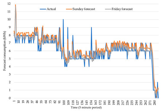
Figure 9.
Actual and forecasted consumption for 13 April 2019.
6. Conclusions
This paper proposes a forecasting application using real time energy consumption belonging to an industrial building and collected for five-minute periods. The forecasts are supported with the artificial neural network (ANN) algorithm and two error metrics using the Python language and the tensorflow library.
The proposed methodology includes features that have been adapted to the specific behavior of an industrial facility. The cleaning operations rescale data to a new version, featuring similar contents with more reliable aspects suitable to be used by forecasting techniques. Additionally, the visualization of data is an area studied with detail in the cleaning version, an aspect that was difficult to be processed in the raw version. The reduced process applied to the dimension of data is a study with great relevance that discards history that might decrease the accuracy of forecast tasks.
The obtained forecasting results for the different architecture options show that by using a higher number of neurons, the accuracy obtained is higher, despite requiring more processing time efforts. It is also noted that if the number of neurons is big enough, then a higher number of neurons provides more accurate forecasts. The forecast results split for the different days of the weeks show forecast improvements featured by a decrease in the forecast error. This means that the proposed method of re-training the ANN at the end of each day is very adequate for this type of electricity consuming facility.
Author Contributions
Conceptualization, P.F. and Z.V.; Data curation, D.R., Z.V., and R.C.; Formal analysis, D.R.; Funding acquisition, P.F., Z.V., and R.C.; Investigation, D.R. and P.F.; Methodology, D.R., P.F., and Z.V.; Project administration, P.F., Z.V., J.M., and R.C.; Resources, P.F. and Z.V.; Software, D.R.; Supervision, P.F. and Z.V.; Validation, D.R., P.F., Z.V., J.M., and R.C.; Visualization, D.R. and P.F.; Writing—original draft, D.R., P.F., and Z.V.; Writing—review and editing, D.R., P.F., Z.V., J.M., and R.C. All authors have read and agreed to the published version of the manuscript.
Funding
This work has received funding from Portugal 2020 under the SPEAR project (NORTE-01-0247-FEDER-040224), in the scope of the ITEA 3 SPEAR Project 16001, from FEDER Funds through the COMPETE program and from National Funds through FCT under the project UIDB/00760/2020 and CEECIND/02887/2017.
Conflicts of Interest
The authors declare no conflict of interest.
References
- Li, X.; Gao, L.; Wang, G.; Gao, F.; Wu, Q. Investing and pricing with supply uncertainty in electricity market: A general view combining wholesale and retail market. China Commun. 2015, 12, 20–34. [Google Scholar] [CrossRef]
- Hauteclocque, A. Legal uncertainty and competition policy: The case of long-term vertical contracting by dominant firms in the EU electricity markets. In Proceedings of the 2008 5th International Conference on the European Electricity Market, Lisboa, Portugal, 28–30 May 2008; pp. 1–8. [Google Scholar]
- Faria, P.; Vale, Z. A Demand Response Approach to Scheduling Constrained Load Shifting. Energies 2019, 12, 1752. [Google Scholar] [CrossRef]
- Zhou, B.; Yan, J.; Yang, D.; Zheng, X.; Xiong, Z.; Zhang, J. A Regional Smart Power Grid Distribution Transformer Planning Method Considering Life Cycle Cost. In Proceedings of the 2019 4th International Conference on Intelligent Green Building and Smart Grid (IGBSG), Yi Chang, China, 6–9 September 2019; pp. 612–615. [Google Scholar]
- Faria, P.; Vale, Z. Demand response in electrical energy supply: An optimal real time pricing approach. Energy 2011, 36, 5374–5384. [Google Scholar] [CrossRef]
- Noppakant, A.; Plangklang, B.; Marsong, S. The Study of Challenge and Issue of Building Demand Response. In Proceedings of the 2019 International Conference on Power, Energy and Innovations (ICPEI), Pattaya, Thailand, 16–18 October 2019; pp. 4–7. [Google Scholar]
- Zhou, Q.; Guan, W.; Sun, W. Impact of demand response contracts on load forecasting in a smart grid environment. In Proceedings of the 2012 IEEE Power and Energy Society General Meeting, San Diego, CA, USA, 22–26 July 2012; pp. 1–4. [Google Scholar]
- Al Hadi, A.; Silva, C.; Hossain, E.; Challoo, R. Algorithm for Demand Response to Maximize the Penetration of Renewable Energy. IEEE Access 2020, 8, 55279–55288. [Google Scholar] [CrossRef]
- Bhuiyan, S.M.A.; Khan, J.F.; Murphy, G.V. Big data analysis of the electric power PMU data from smart grid. In Proceedings of the SoutheastCon 2017, Charlotte, NC, USA, 30 March–2 April 2017; pp. 1–5. [Google Scholar]
- Abrishambaf, O.; Faria, P.; Vale, Z. Application of an optimization-based curtailment service provider in real-time simulation. Energy Inform. 2018, 1, 3. [Google Scholar] [CrossRef]
- Aggarwal, C.C. Data Classification: Algorithms and Applications; CRC Press: Boca Raton, FL, USA, 2015. [Google Scholar]
- Suzuki, K. Artificial Neural Networks—Architectures and Applications; Intech: London, UK, 2013. [Google Scholar]
- Kramer, O. Dimensionality Reduction with Unsupervised Nearest Neighbors; Springer: Berlin/Heidelberg, Germany, 2013. [Google Scholar]
- Cunningham, P.; Delany, S.J. k-Nearest Neighbour Classifiers; UCD: Dublin, Ireland, 2007. [Google Scholar]
- Cutler, A.; Cutler, D.R.; Stevens, J.R. Ensemble Machine Learning: Methods and Applications; Springer: Berlin/Heidelberg, Germany, 2012. [Google Scholar]
- Sahay, K.B.; Singh, K. Short-Term Price Forecasting by Using ANN Algorithms. In Proceedings of the 2018 International Electrical Engineering Congress (iEECON), Krabi, Thailand, 7–9 March 2018; pp. 1–4. [Google Scholar]
- Bhatt, G.A.; Gandhi, P.R. Statistical and ANN based prediction of wind power with uncertainty. In Proceedings of the 2019 3rd International Conference on Trends in Electronics and Informatics (ICOEI), Tirunelveli, India, 23–25 April 2019; pp. 622–627. [Google Scholar]
- Mamun, M.A.; Nagasaka, K. Artificial neural networks applied to long-term electricity demand forecasting. In Proceedings of the Fourth International Conference on Hybrid Intelligent Systems (HIS’04), Kitakyushu, Japan, 5–8 December 2004; pp. 204–209. [Google Scholar]
- Bracale, A.; Falco, P.; Carpinelli, G. Comparing Univariate and Multivariate Methods for Probabilistic Industrial Load Forecasting. In Proceedings of the 2018 5th International Symposium on Environment-Friendly Energies and Applications (EFEA), Rome, Italy, 24–26 September 2018; pp. 1–6. [Google Scholar]
- Ramos, D.; Faria, P.; Vale, Z. Electricity Consumption Forecast in an Industry Facility to Support Production Planning Update in Short Time. In Proceedings of the 2020 IEEE International Conference on Environment and Electrical Engineering and 2020 IEEE Industrial and Commercial Power Systems Europe (EEEIC/I&CPS Europe), Madrid, Spain, 9–12 June 2020; pp. 1–6. [Google Scholar]
- Keras. Available online: https://www.tensorflow.org/guide/keras (accessed on 29 May 2020).
- Bracale, A.; Carpinelli, G.; Falco, P.; Hong, T. Short-term industrial load forecasting: A case study in an Italian factory. In Proceedings of the 2017 IEEE PES Innovative Smart Grid Technologies Conference Europe (ISGT-Europe), Torino, Italy, 26–29 September 2017; pp. 1–6. [Google Scholar]
- Paulus, M.; Borggrefe, F. The potential of demand-side management in energy-intensive industries for electricity markets in Germany. Appl. Energy 2011, 88, 432–441. [Google Scholar] [CrossRef]
- Berk, K.; Hoffmann, A.; Muller, A. Probabilistic forecasting of industrial electricity load with regime switching behavior. Int. J. Forecast. 2018, 34, 147–162. [Google Scholar] [CrossRef]
- Huang, X.; Hong, S.; Li, Y. Hour-Ahead Price Based Energy Management Scheme for Industrial Facilities. IEEE Trans. Ind. Inform. 2017, 13, 2886–2898. [Google Scholar] [CrossRef]
- Gooijer, J.; Hyndman, R. 25 years of time series forecasting. Int. J. Forecast. 2006, 22, 443–473. [Google Scholar] [CrossRef]
- Sánchez-Sánchez, P.A.; García-González, J.R.; Coronell, L.H.P. Encountered Problems of Time Series with Neural Networks: Models and Architectures. In Recent Trends in Artificial Neural Networks-From Training to Prediction; Intech: London, UK, 2019. [Google Scholar]
- Naim, I.; Mahara, T.; Idrisi, A.R. Effective Short-Term Forecasting for Daily Time Series with Complex Seasonal Patterns. Procedia Comput. Sci. 2018, 132, 1832–1841. [Google Scholar] [CrossRef]
- Mahalakshmi, G.; Sridevi, S.; Rajaram, S. A survey on forecasting of time series data. In Proceedings of the 2016 International Conference on Computing Technologies and Intelligent Data Engineering, Kovilpatti, India, 7–9 January 2016; pp. 1–8. [Google Scholar]
- Tealab, A. Time series forecasting using artificial neural networks methodologies: A systematic review. Future Comput. Inform. J. 2018, 3, 334–340. [Google Scholar] [CrossRef]
- Ashour, M.A.H.; Abbas, R.A. Improving Time Series’ Forecast Errors by Using Recurrent Neural Networks. In Proceedings of the 7th International Conference on Software and Computer Applications, Kuantan, Malaysia, 8–10 February 2018; pp. 229–232. [Google Scholar]
- Wan, R.; Mei, S.; Wang, J.; Liu, M.; Yang, F. Multivariate Temporal Convolutional Network: A Deep Neural Networks Approach for Multivariate Time Series Forecasting. Electronics 2019, 8, 876. [Google Scholar] [CrossRef]
- Bontempi, G.; Taieb, S.B.; Borgne, Y.L. Machine Learning Strategies for Time Series Forecasting. In European Business Intelligence Summer School; Springer: Berlin/Heidelberg, Germany, 2012; pp. 62–77. [Google Scholar]
- Nor, M.E.; Safuan, H.M.; Shab, N.F.M.; Abdullah, M.A.A.; Mohamad, N.A.I.; Muhammad, L. Neural network versus classical time series forecasting models. In Proceedings of the AIP Conference Proceedings, Vladivostok, Russia, 18–22 September 2017; Volume 1842. [Google Scholar]
- Martínez-Álvarez, F.; Troncoso, A.; Riquelme, J. Recent Advances in Energy Time Series Forecasting. Energies 2017, 10, 809. [Google Scholar] [CrossRef]
- Ponce-Flores, M.; Frausto-Solís, J.; Santamaría-Bonfil, G.; Pérez-Ortega, J.; González-Barbosa, J. Time Series Complexities and Their Relationship to Forecasting Performance. Entropy 2020, 22, 89. [Google Scholar] [CrossRef]
- Divina, F.; Torres, M.; Vela, F.; Noguera, J. A Comparative Study of Time Series Forecasting Methods for Short Term Electric Energy Consumption Prediction in Smart Buildings. Energies 2019, 12, 1934. [Google Scholar] [CrossRef]
- Martínez-Álvarez, F.; Troncoso, A.; Cortés, G.; Riquelme, J. A Survey on Data Mining Techniques Applied to Electricity-Related Time Series Forecasting. Energies 2015, 8, 13162–13193. [Google Scholar] [CrossRef]
© 2020 by the authors. Licensee MDPI, Basel, Switzerland. This article is an open access article distributed under the terms and conditions of the Creative Commons Attribution (CC BY) license (http://creativecommons.org/licenses/by/4.0/).