Optimization of Voltage Unbalance Compensation by Smart Inverter

Abstract

This paper presents a compensation method for unbalanced voltage through active and reactive power control by utilizing a smart inverter that improves the voltage unbalance index and detects an unbalanced state of voltage magnitude and phase, and thus enhances power quality by minimizing the voltage imbalance. First of all, this paper presents an analysis of a mathematical approach, which demonstrates that the conventional voltage unbalanced factor (VUF) using the symmetrical component cannot correctly detect the imbalanced state from index equations; and by only minimizing the VUF value, it cannot establish a balanced condition for an unbalanced state of the voltage profile. This paper further discusses that intermittent photovoltaic (PV) output power and diversified load demand lead to an unexpected voltage imbalance. Therefore, considering the complexity of unbalanced voltage conditions, a specific load and an PV profile were extracted from big data and applied to the distribution system model. The effectiveness of the proposed scheme was verified by comparing VUF indices and controlling the active and reactive power of a smart inverter through a numerical simulation.

1. Introduction

A power system is designed based on energy security, economic efficiency, and safety requirements at the generation, transmission, and distribution level. Technical challenges associated with system stabilities and power quality have been gaining more attention in recent years due to the massive implementation of renewable energy sources (RES) which include voltage deviation and fluctuation [1,2] by photovoltaic (PV) output power, energy losses, decreasing rate of plant utilization and synchronizing power, phase balancing, etc. For power utilities and customers, the system voltage at the node-end is one of the important indexes for measuring the power quality [3,4]. Despite a large number of power quality indicators [4], previous voltage adjustment is not considered for phase unbalance of the voltage in the optimization problem [5,6,7,8,9]. This consideration could be different on the voltage level, and if the scale is different, appropriate indicators to be applied may also differ. However, as reported in [9,10,11] the compensation devices’ control magnitude of voltage must be maintained within an appropriate range as power security. This paper focuses on the voltage imbalance problem accompanying heavy load and unbalanced connection of RES, not only considering voltage magnitude but also phase unbalance.

Voltage imbalance is often caused by load imbalance or line impedance conditions [12,13,14], except in transient cases such as faults [15]. When the unbalanced state continues, current will flow through the neutral wire, which may lead to a miss-recognition of the fault; then the circuit breaker may be opened, causing power outages. The induction machine is affected by the unbalanced voltage that will diminish the power factor and increases the losses, causing the windings to get damaged due to excess heat [16]. When an unbalanced voltage is supplied to powered electronic equipment, it causes harmonics, which causes problems such as heat, losses, and a reduction in the lifespan of the equipment [17,18]. On the other hand, in the smart power distribution grid, the diversity of loads including power generation increases, and the uncertainty associated with RES causes an imbalance in the $abc$-phase (3$\varphi$) voltage in the distribution system. In recent years, the three-phase imbalance problem has been studied as an unbalance problem [19] derived from power generation and imbalance accompanying an unbalanced load. Furthermore, the unbalance exerted by the linear load and the unbalance exerted by the nonlinearity are actively discussed in the field of power electronics [20]. The control method for a two-inverter interconnected power system with series and parallel connections is well discussed in [21,22]. Each inverter function is separated as—the shunt inverter is widely proposed for control power flow (both active and reactive power) for distributed generators (DGs). On the other hand, voltage and line current are balanced by series inverter parts. Unbalance is compensated by adjusting a negative sequence voltage. Further, on-load tap changing (OLTC) transformers, series capacitors, and shunt reactors have been used for a years for voltage fluctuation mitigation. In addition, mitigation voltage variations by power electronic devices have been reported in [23,24]—e.g., active and passive power filters [25,26], the static var compensator (SVC) [21], and unified power quality conditioners (UPQC) [27]. The major drawback of UPQC and SVC is they are costly.

This paper primarily focuses on three-phase unbalanced voltage compensation utilizing a smart inverter for three-phase unbalanced voltage compensation. The smart inverter can provide reactive power (volt-var) control using margin of inverter capacity [28,29,30]. The active power (volt-watt) can also be adjusted, but in general, suppresses the RES power output to minimize any adverse impacts on the grid performance. Moreover, by combining a smart inverter with a storage battery, volt-watt control can be effectively performed [29,31].

The significant contributions of this paper are listed below:

(i)

Development of a mathematical approach to elucidate the conventional voltage imbalance index and undetectable unbalance state.

(ii)

Detailed analysis on impact of RES causing undetectable unbalance (e.g., voltage unbalance) in the distribution system.

(iii)

Application of a heuristic optimization method based on particle swarm optimization (PSO) to balance voltage phase and magnitude unbalances.

(iv)

Analysis of big data to reduce the large volume of data and to extract essential features of data without deficiencies by using k-means clustering.

(v)

Advancing the application of the smart inverter, in particular for active and reactive power control, as a three-phase unbalanced compensation.

The remaining sections of the paper are organized as follows. Voltage unbalance conditions and the symmetrical component with a detailed discussion are provided in Section 2 and Section 3, respectively. Section 4 presents the optimization formulation. Section 5 explains big data processing for load demand and PV generation profile. In Section 6, the effectiveness of the proposed method is presented with a comparative analysis. Finally, the conclusions are drawn in Section 7.

2. Unbalance Assessment

The voltage imbalance needs to be appropriately evaluated and controlled; however, the symmetrical components method, used in general, cannot correctly detect the unbalanced state. This section discusses voltage magnitude imbalance and phase imbalance.

The three-phase voltage can be visualized using a phasor diagram, and the case of the unbalanced state is shown in Figure 1. The voltage unbalanced factors ($VUFs$) of unbalanced states A ($\{V_a,V_b,V_c\}=\{1.0+j0.1,-0.57-j0.88,-0.61+j0.86\}$) and B ($\{V_a,V_b,V_c\}=\{1.0-j0.1,-0.43-j0.85,-0.39+j0.87\}$) are 3.5% and 3.7% (see Section 3 for $VUF$ calculation). Phasor diagrams are practical as a visualization method for seeing symmetric vectors; however, it is not easy to judge the occurrence of unbalances. Namely, it is difficult to determine the amount of voltage compensation. Therefore, the imbalance rate evaluation by vector addition using the symmetrical component method is presented in this paper by graphical interpretation.

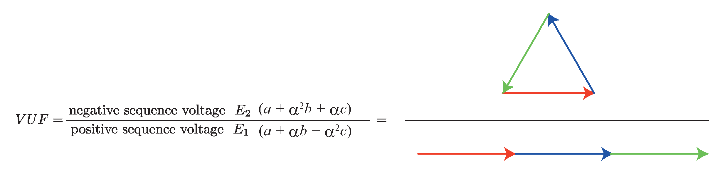
2.1. Voltage Magnitude Imbalance

In the static simulation, it simply considers the voltage imbalance of the magnitude. The unbalance of each phase also includes phase imbalance, and generally, the $VUF$ index is used; however, in this index, the imbalance of the magnitude of the voltage is not directly expressed. Although it is possible to verify the voltage magnitude unbalance indirectly, it is necessary to evaluate the imbalance of the voltage magnitude directly. Thus, this study utilized the IEEE 123 bus test system (in which single-phase, two phases, and three phases are mixed) for the purpose of simulation, and the respective magnitude of voltage unbalance factor ($MVUF$) is defined as follows [32]:

$$MVU{F}_i=\left\{\begin{array}{cc}\hfill V_{mvuf,3\varphi }& =\frac{|{\dot{V}}_{max,i}|-|{\dot{V}}_{min,i}|}{|{\dot{V}}_{ave}|}\left(threephase\right)\hfill \\ \hfill V_{mvuf,2\varphi }& =\frac{|{\dot{V}}_{max,i}|-|{\dot{V}}_{min,i}|}{|{\dot{V}}_{ave}|}\left(twophase\right)\hfill \\ \hfill V_{mvuf,1\varphi }& =\frac{|{\dot{V}}_i|}{V_{base}}\left(singlephase\right)\hfill \end{array}\right.$$

(1)

where $MVU{F}_i$ is the magnitude of voltage unbalance factor at the node i. $1\varphi ,2\varphi ,3\varphi$ represent single, two, and three phases, respectively. $MVU{F}_i$ is selected from $V_{mvuf,1\varphi },V_{mvuf,2\varphi },V_{mvuf,3\varphi }$ configuration of node i. ${\dot{V}}_{min,i},{\dot{V}}_{max,i}$ are the minimum and maximum voltage at node i. $V_{base}$ is base voltage; here, $V_{base}=1.0$ (p.u.).

2.2. Voltage Phase Imbalance

An unbalance factor of voltage magnitude is used for general static simulation, whereas phase imbalance is mainly used when focusing in the field of power electronics and instantaneous values. The phase unbalances can be detected from the phase difference at phasors. In the case of a load including many inductance components and capacitor components, the phase difference becomes large. Additionally, a minute voltage imbalance is caused by the inductance component which is included in the line.

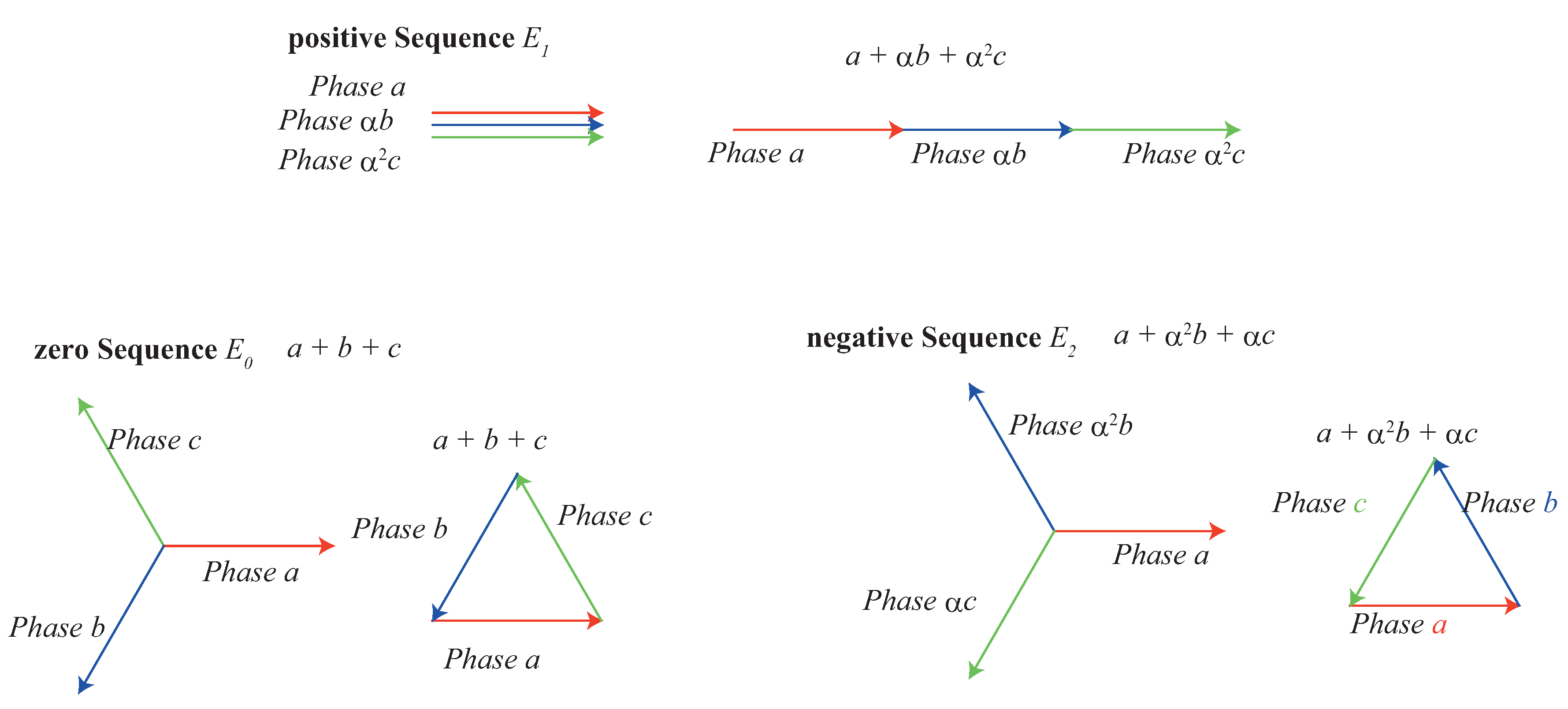
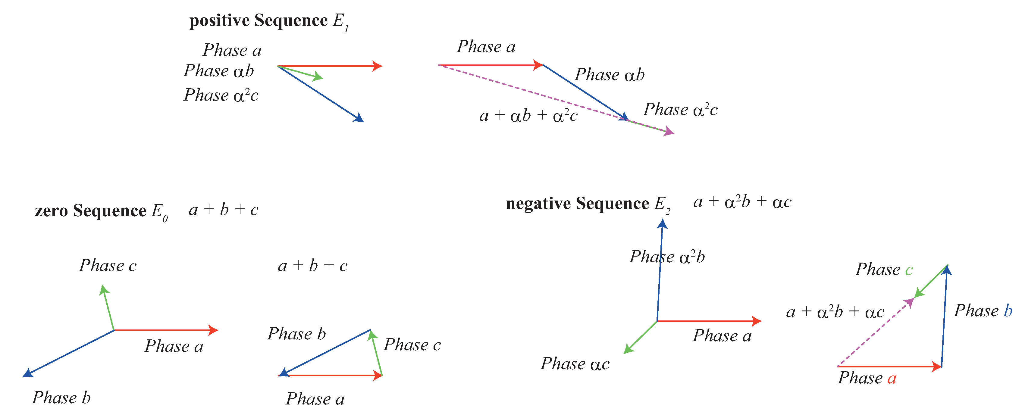
3. Symmetrical Component

The symmetric components method is thought to be indispensable for the understanding of the three-phase power system. The three components, zero, positive, and negative sequence converted from three-phase voltages by the symmetrical components method are shown in Figure 2. The conversion equation is given as

$${\displaystyle \begin{array}{cc}\hfill \left[\begin{array}{c}{\dot{E}}_0\\ {\dot{E}}_1\\ {\dot{E}}_2\end{array}\right]& =\frac{1}{3}\left[\begin{array}{ccc}1& 1& 1\\ 1& \alpha & {\alpha }^2\\ 1& {\alpha }^2& \alpha \end{array}\right]\left[\begin{array}{c}{\dot{V}}_a\\ {\dot{V}}_b\\ {\dot{V}}_c\end{array}\right]\hfill \end{array}}$$

(2)

where $V_{\{a,b,c\}}$ is each phase voltage, and $E_{\{0,1,2\}}$ represents zero, positive, and negative sequence voltages in symmetrical component transform. Here, $\alpha$ is vector operator; it is defined as $\alpha \equiv e^{j\frac{2\pi }{3}}=-\frac{1}{2}+j\frac{\sqrt{3}}{2}$. This operator $\alpha$ rotates a phasor by 120 degree. The Figure 2 shows the balanced three-phase voltage, which means zero and negative-sequence components become zero in balanced situation. Since the unbalance rate is defined as $VUF=E_2/E_1$ [3], the graphical interpretation of the unbalance rate is shown in Figure 3. Under balanced $VUF$ definition, the numerator becomes zero; in other words, the component of the negative-sequence phase is an index of the unbalance rate.

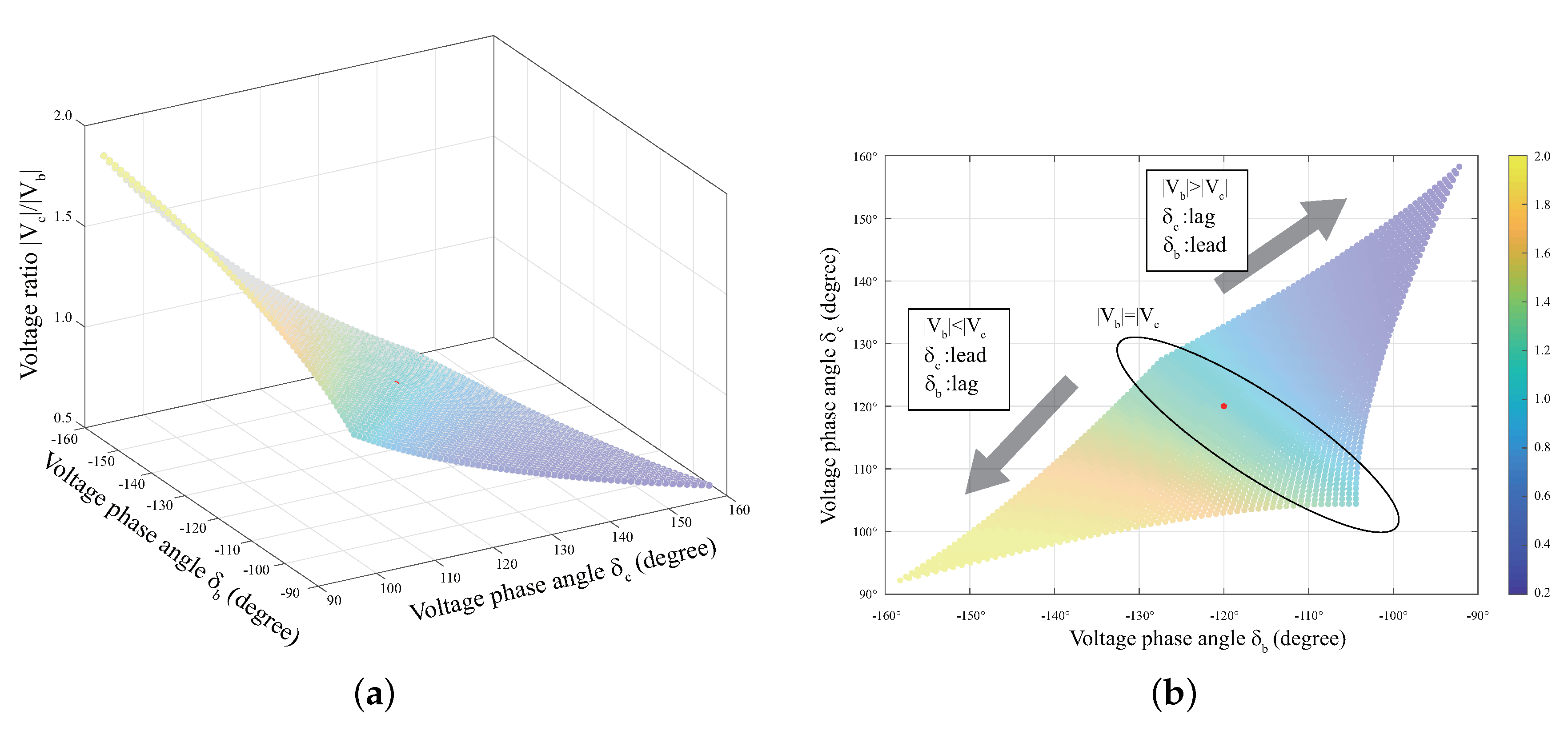
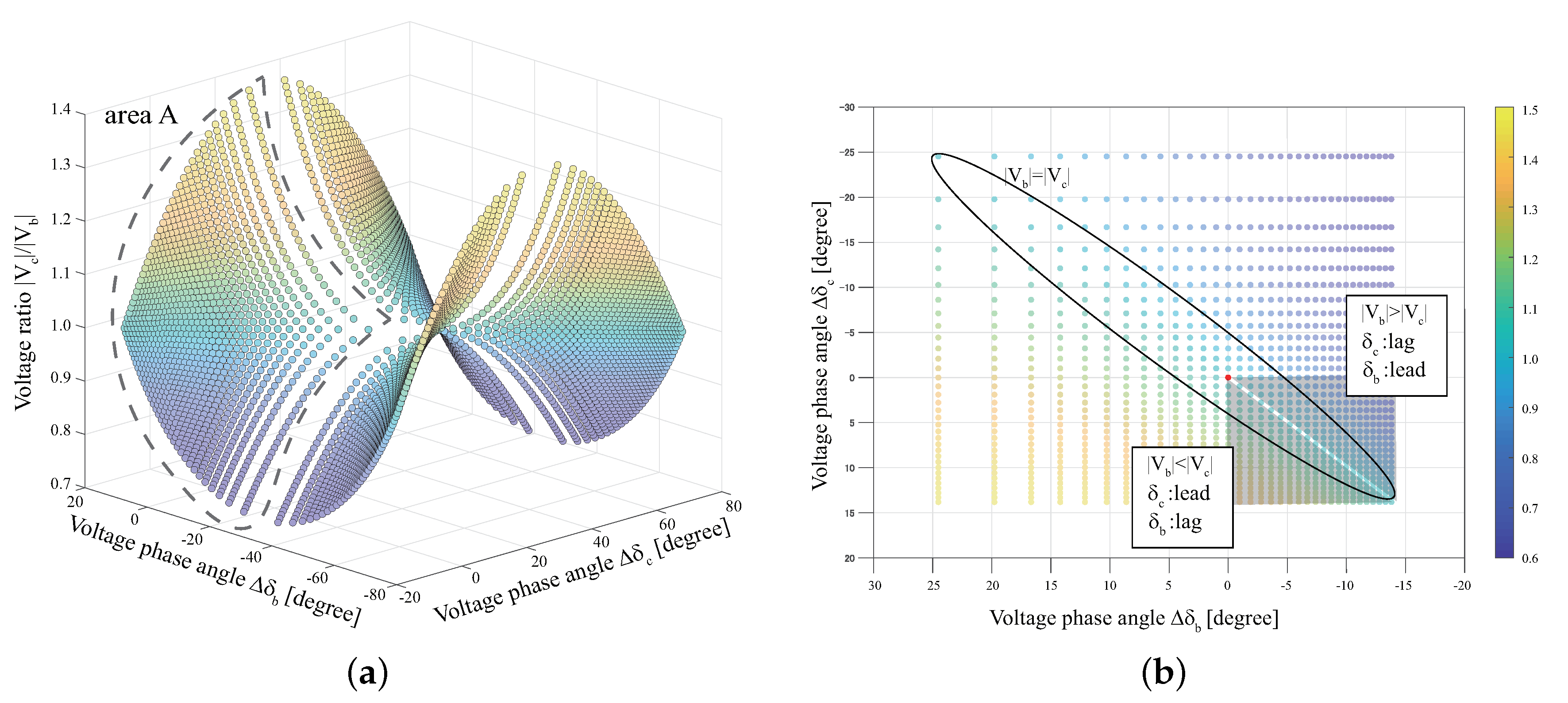
3.1. Unbalanced Situations at Symmetrical Components

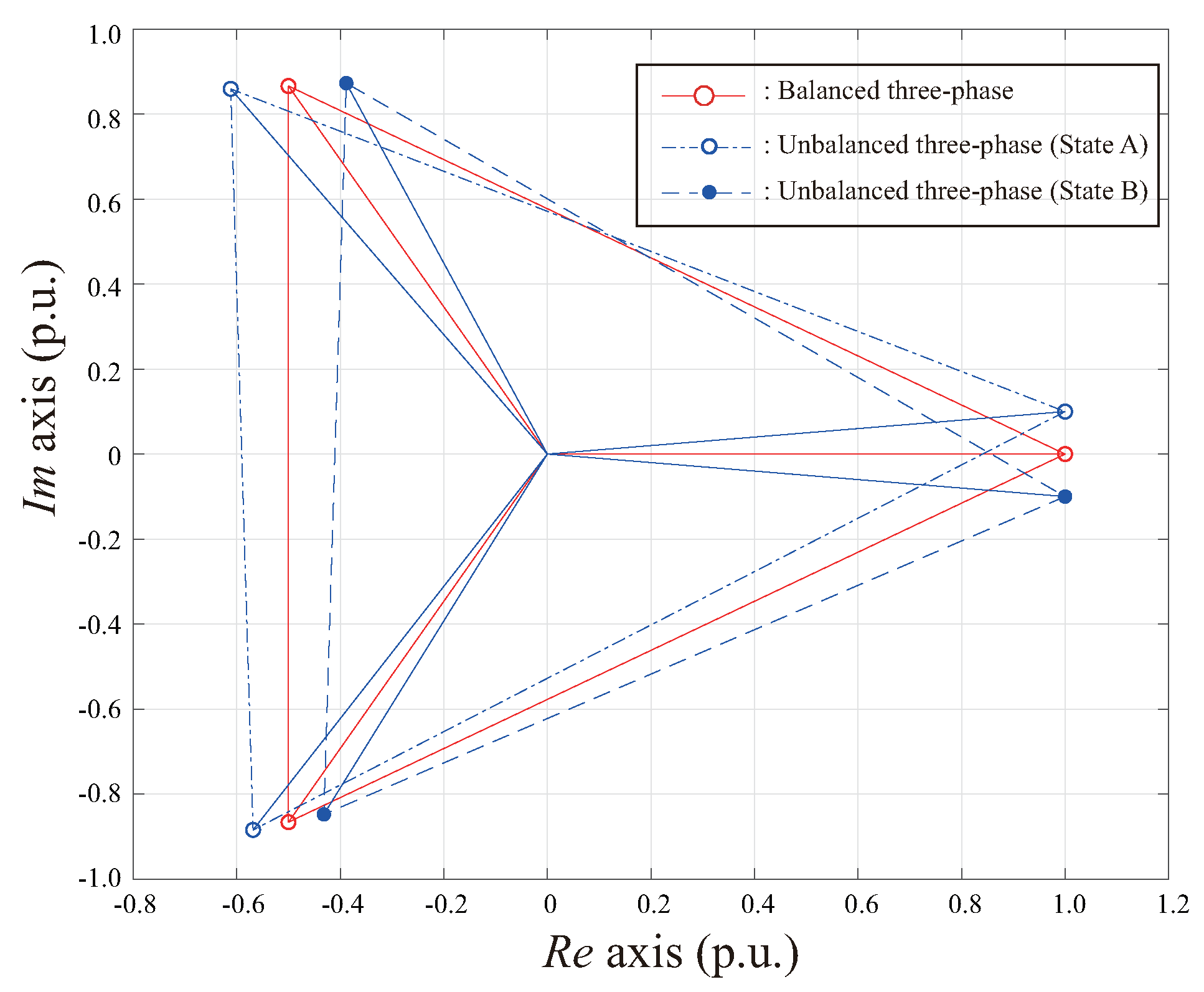
An extreme example of causing unbalance is shown in Figure 4. An unbalance is caused when at least one phase or magnitude of voltage is unbalanced. Since the line impedance is kept in balance, the imbalance of the voltage can be understood as the current (power) imbalance causes. Since it is practically impossible for the positive sequence voltage to become zero, if the negative sequence voltage is not zero, the voltage causes an imbalance. Thus, voltage unbalance state is detected as shown in Figure 5.

3.2. Unbalanced but $VUF=0$ Situations

Ordinal $VUF$ which is defined as a three-phase unbalance rate may be $VUF=0$ even in a situation where an imbalance occurs. In the d–q axis transformation as well, an imbalance may occur even when the imbalance amount is zero ($V_q=0$) (when phase b and c are line-symmetric with respect to the horizontal axis). In the case of using the d–q transformation mainly in the case of controlling the output of the generator and controlling the motor, since feedback control of the frequency is included in addition to the control to set the q axis to zero, the unbalance compensation is partly possible. However, when a large amount of RES is interconnected, the load suddenly changes to power generation, so the phase changes in complex manner. In other words, an unbalanced state may not be properly detected by normal control and an indicator, and imbalance compensation may not be possible.

Next, the situation wherein $VUF=0$ but is in an unbalanced state is explained. The $VUF=0$ means that the negative-sequence is zero. This corresponds to the case where phase b is delayed and the phase c will lead, and vice-versa. Figure 6 shows the transformed phasor of unbalanced but $VUF=0$ condition. A graphical representation of $VUF$ is shown in Figure 7. Since the part of the numerator becomes zero, there is a situation in which it is recognized as no apparent imbalance.

3.3. Undetectable Voltage Unbalanced Condition

In this paper, an unbalanced but $VUF=0$ situation is called “undetectable unbalanced condition.” A mathematical approach reveals the undetectable unbalanced condition. The negative sequence voltage is given as

$${\dot{E}}_2={\dot{V}}_a+{\alpha }^2{\dot{V}}_b+\alpha {\dot{V}}_c$$

(3)

Here, phase a voltage is the base (${\dot{V}}_a=1+j\times 0$); thus, Equation (3) is expressed as

$${\dot{V}}_2=1+{\dot{V}}_b\times \left(cos\frac{4}{3}\pi +jsin\frac{4}{3}\pi \right)+{\dot{V}}_c\times \left(cos\frac{2}{3}\pi +jsin\frac{2}{3}\pi \right)$$

(4)

The variables of Equation (4) can be separated as

$$\left\{\begin{array}{cc}\hfill V_{2,\mathrm{Re}}& =1+|{\dot{V}}_b|cos({\delta }_b-\frac{2}{3}\pi )+\left|{\dot{V}}_c\right|cos({\delta }_c+\frac{2}{3}\pi )=0\hfill \\ \hfill V_{2,\mathrm{Im}}& =|{\dot{V}}_b|sin({\delta }_b-\frac{2}{3}\pi )+\left|{\dot{V}}_c\right|sin({\delta }_c+\frac{2}{3}\pi )=0\hfill \end{array}\right.$$

(5)

where $V_{2,\mathrm{Re}}$ and $V_{2,\mathrm{Im}}$ are vales of real and imaginary numbers of Equation (4), and ${\delta }_b$ and ${\delta }_c$ are voltage angles of b and c phase. The cross point of implicit functions of Equation (5) shows the voltage state at point of undetectable unbalanced condition ($E_2=0$). The implicit functions when the voltages magnitude values of b and c phase are changed from 0.7 p.u. to 1.3 p.u. are shown in Figure 8. The green dots plot represents actual balanced point, and other red points plot are undetectable unbalanced points. The condition is innumerable and unbalanced but recognized as balanced points on the symmetrical component method, as shown in Figure 8.

In order to confirm the phenomenon in more detail, the voltage magnitude ratio ($|{\dot{V}}_c|/|{\dot{V}}_b|$) was set to the z axis or color bar axis, as shown in Figure 9, which was depicted by extracting the red dots in Figure 8. When the PV equipment is connected to the b phase and the load demand is connected to the c phase, it belongs to the point on the right side of Figure 9a, while when the equipment of the b and c phases is interchanged, it belongs to the left side of Figure 9b. In other words, the distribution system includes the penetration of PV and the customer randomly connects the PV system to each phase, which may cause undetected unbalanced conditions to occur frequently.

On the other hand, d–q axis transformation is also frequently used in voltage control, and the transformation verifies whether there are undetected unbalanced voltage conditions in d–q transformation process. The transformation is given by

$$\left[\begin{array}{c}{V}_d\\ V_q\end{array}\right]=\frac{2}{3}\left[\begin{array}{ccc}cos\left(\omega t\right)& cos(\omega t-\frac{2\pi }{3})& cos(\omega t+\frac{2\pi }{3})\\ sin\left(\omega t\right)& sin(\omega t-\frac{2\pi }{3})& sin(\omega t+\frac{2\pi }{3})\end{array}\right]\left[\begin{array}{c}{\dot{V}}_a\\ {\dot{V}}_b\\ {\dot{V}}_c\end{array}\right]$$

(6)

If the q-axis voltage is 0 and the d-axis voltage is a constant value; the three-phase balanced state can be maintained; and we verify whether an unbalanced state exists in such state. Thus, the implicit function is given by

$$\left\{\begin{array}{cc}\hfill V_d& =K\hfill \\ \hfill V_q& =0\hfill \end{array}\right.$$

(7)

Here, constant value K is set to 1. The voltage magnitude values of $|{\dot{V}}_b|$ and $|{\dot{V}}_c|$ are changed from 0.86 p.u. to 1.2 p.u., as is shown in Figure 10. As it can be seen in Figure 10a, there exist four areas but the feasible area is only area A, which is shown in Figure 10b. Note that the angular axis is the differences of angle $\Delta {\delta }_{b,c}$ from the balanced point. Namely, true balanced condition is the plot of $\Delta {\delta }_b=\Delta {\delta }_c=0$.

Similarly, Figure 10 shows undetectable unbalanced conditions. Upper triangular and lower triangular parts of Figure 10b are also similar to the symmetrical component. Thus, an undetectable unbalanced phenomenon exists regardless of the method.

Therefore, in consideration of the control necessary to compensate the recent voltage imbalance, conventional $VUF$ alone is insufficient.

4. Optimization of Voltage Unbalance Compensation

4.1. Formulation for Optimization

The previous section revealed that conventional $VUF$ is not enough for unbalanced detection. The condition for satisfying the voltage equilibrium state is to simultaneously satisfy the following two equations.

Conventional $VUF$

$$VU{F}_1=\frac{E_2}{E_1}$$

(8)

Additional $VUF$

$$VU{F}_2=\frac{E_0}{E_1}$$

(9)

where $E_0$ is zero sequence voltage in the symmetrical component method. These indicators (Equations (8) and (9)) are used in solving the optimization problem together with the voltage magnitude unbalance. To confirm the effectiveness of the unbalance index, it is provided with two objective functions. The following equation is used for three-phase unbalance compensation by conventionally minimizing indices.

Objective function 1

$$f_1=min\sum _{i=1}^{N_{node}}(VU{F}_{1,i}+MVU{F}_i)$$

(10)

where variable i expresses node number, and $N_{node}$ is total node number in the distribution system. In order to ensure optimal planning, it is necessary to minimize both voltage magnitude unbalance and phase unbalance. It is to be noted that for compensating phase imbalance, $VUFs$ ($VU{F}_1$ and $VU{F}_2$) are minimized. Therefore, the proposed objective function consists of minimizing Equations (8), (9), and (1) as follows:

Objective function 2

$$f_2=min\sum _{i=1}^{N_{node}}(VU{F}_{1,i}+VU{F}_{2,i}+MVU{F}_i)$$

(11)

A part of $VU{F}_1$ and $VU{F}_2$ from the objective function $f_2$ guarantees the phase imbalance by minimizing the negative phase voltage and the zero phase voltage, and the purpose of minimizing the $MVUF$ is to compensate for the imbalance of the voltage magnitude, respectively. For optimization, the power flow calculation and several constraints such as battery and inverter output are considered [33]. The inverter is installed at all nodes of the distribution system.

4.2. Optimization Method

This paper presents a metaheuristic optimization method using particle swarm optimization (PSO) for smart inverter operation. The method searches an optimum solution by coordinating the particles in a swarm. The particles share the best position and get updated using shared information, which is expressed by the current position and updated velocity given by

$$v_i(k+1)=w_i\left(k\right)·v_i\left(k\right)+c_1·rand·(pbest\left(i\right)-s_i\left(k\right))+c_2·rand·(gbest-s_i\left(k\right))$$

(12)

$$s_i(k+1)=s_i\left(k\right)+c_i\left(k\right)$$

(13)

Equation (12) is velocity update equation. $v_i\left(k\right)$ is velocity of i-th particle at generation k. $s_i\left(k\right)$ is current position. Acceleration constants $c_1,c_2$ are set as 1.4. $rand$ is random number with range $[0,1]$. $pbest$ and $gbest$ are the best positions of the self particle and particle swarm. Particles’ positions are updated by Equation (13). Furthermore, to improve the convergence performance of PSO, the adaptive inertia $w_i$ is applied as follows.

$$w_i(k+1)=w\left(0\right)+(w\left(n_k\right)-w\left(0\right))\times \frac{e^{m_i\left(k\right)}-1}{e^{m_i\left(k\right)}+1}$$

(14)

$$m_i\left(k\right)=\frac{gbest-current}{gbest+current}.$$

(15)

Here, the inertia values $w_i$ and $n_k$ are particles that adjust the inertia of each particle, n and $m_i$ in generation k.

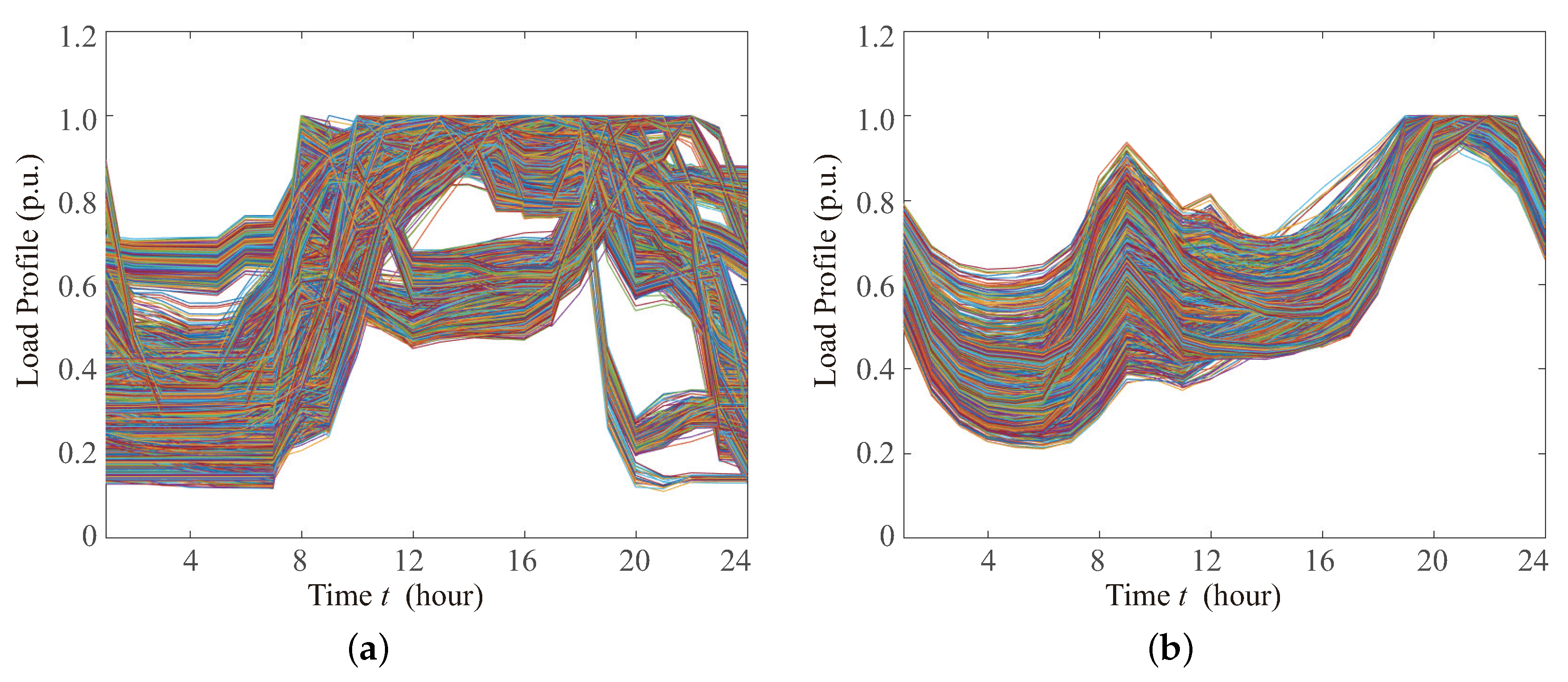
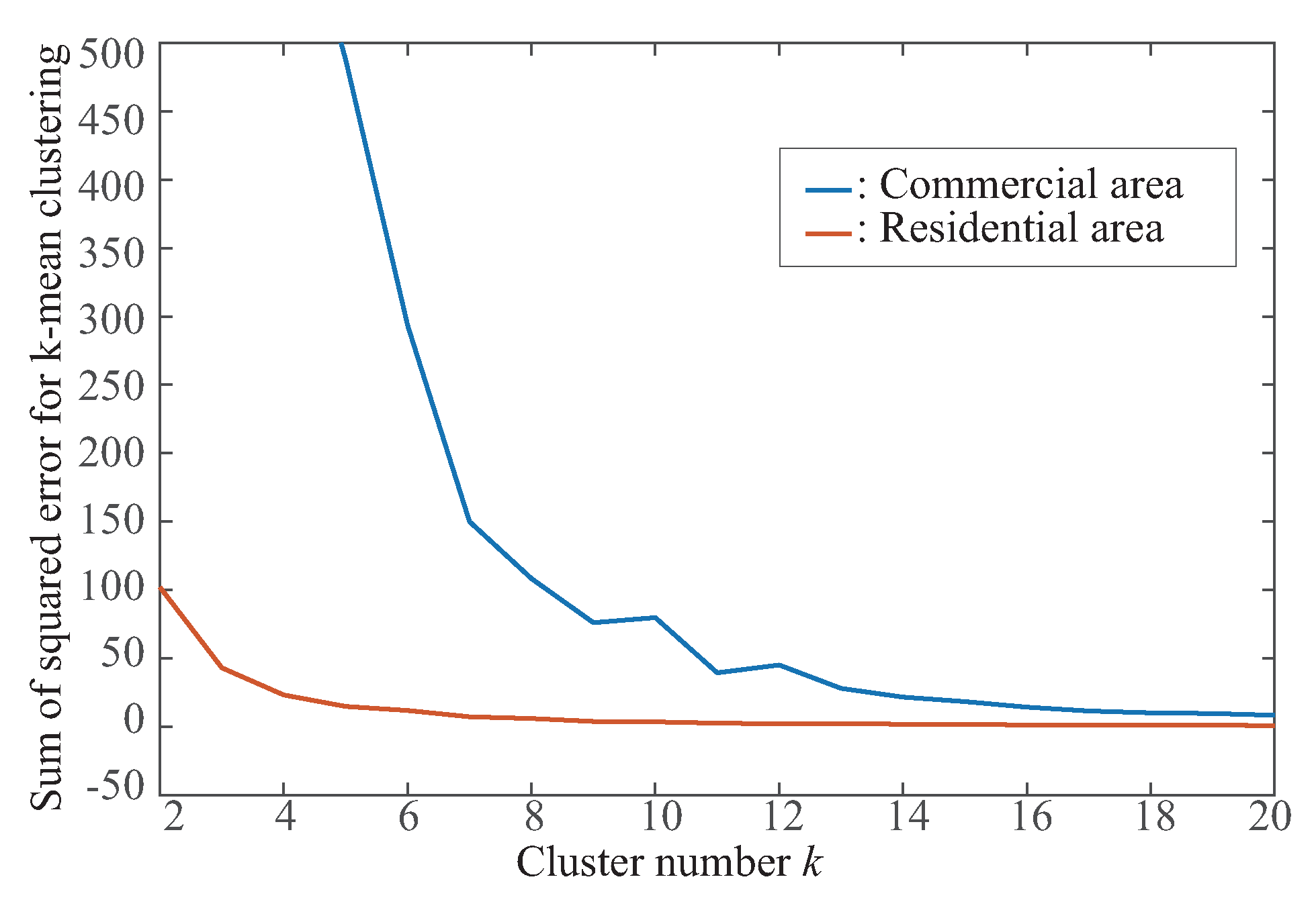
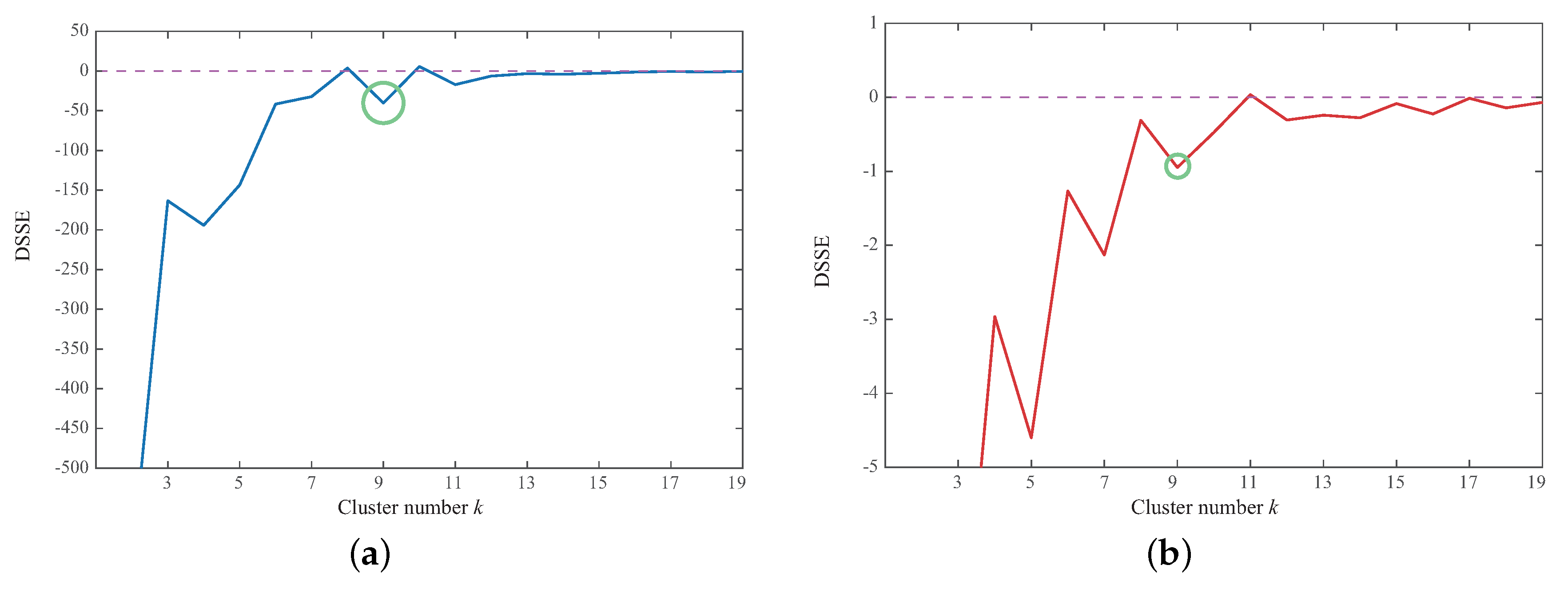
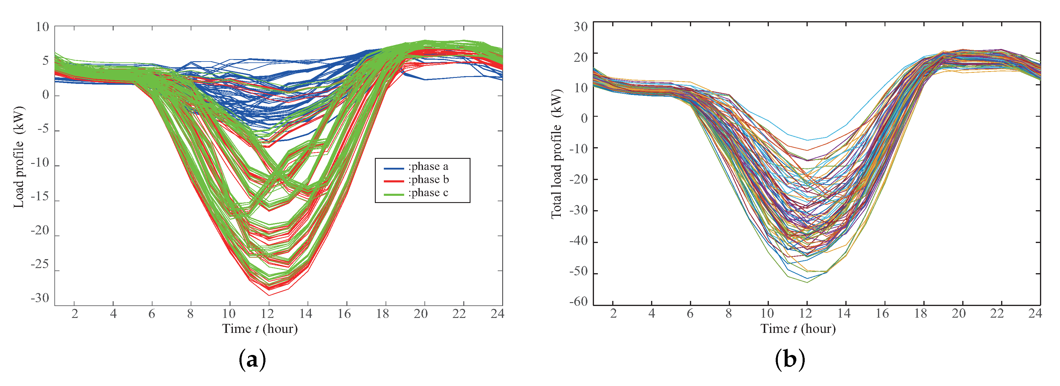
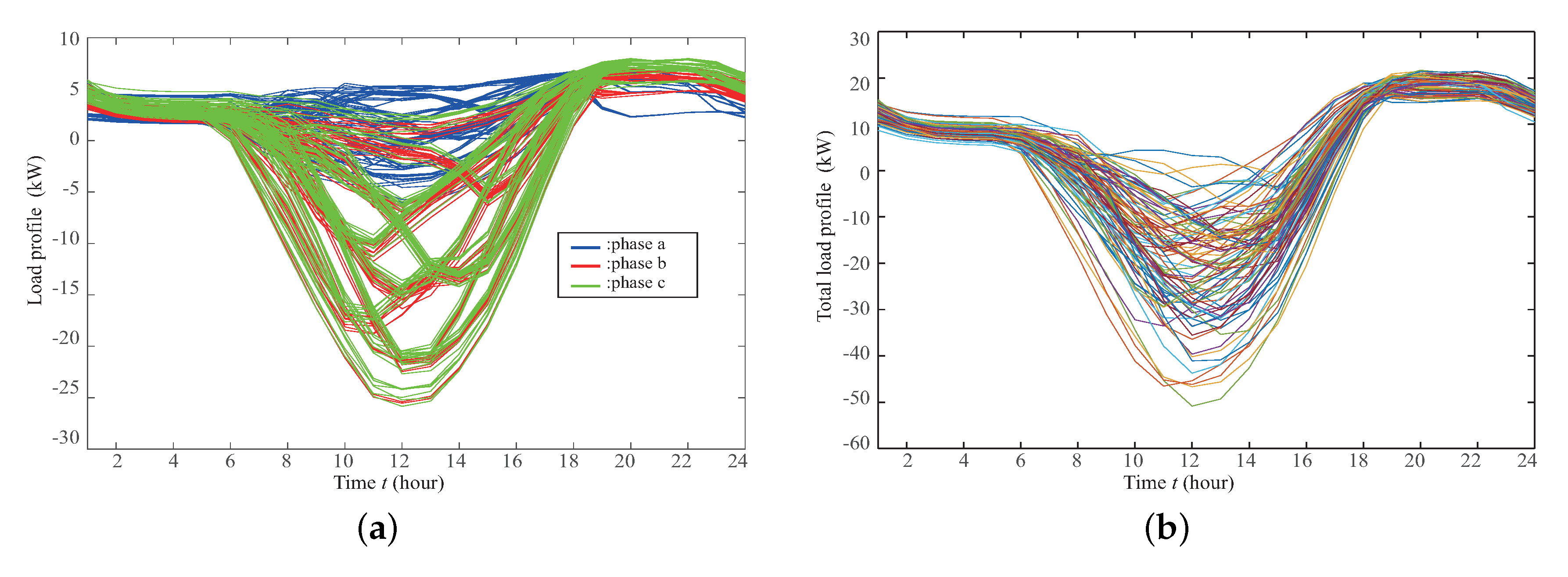
5. A Big Data Approach for a Power System: Load Selection

In electric power systems, the amount of data to be targeted is huge, and the tendencies toward data collection and open-data are increasing. This has further brought complexity into the analysis, which tends to be complicated as the sensor converts everything into data.

Acquiring and applying all the load profiles including uncertainty becomes more difficult as the system size increases. However, it is possible to extract the characteristic of load patterns using clustering acquired from various loads and to reduce the load calculation by using the load profile. This paper uses 24-h-period data set of 14,976 commercial load profiles (see Figure 11a) and 3046 residential load profiles (see Figure 11b). The data of commercial and residential load profiles were acquired from openEI website [34]. The base-load model is based on America B10 Benchmark and the analysis of the load is available at [35]. However, numerous data are time consuming for analysis, and there is a limit in improving the accuracy for the time-period. When processing with big data, it is important to reduce the amount of data and extract important features without deficiencies. Therefore, the feature quantity of the load was extracted using k-means clustering, and how cluster number k was determined is described below.

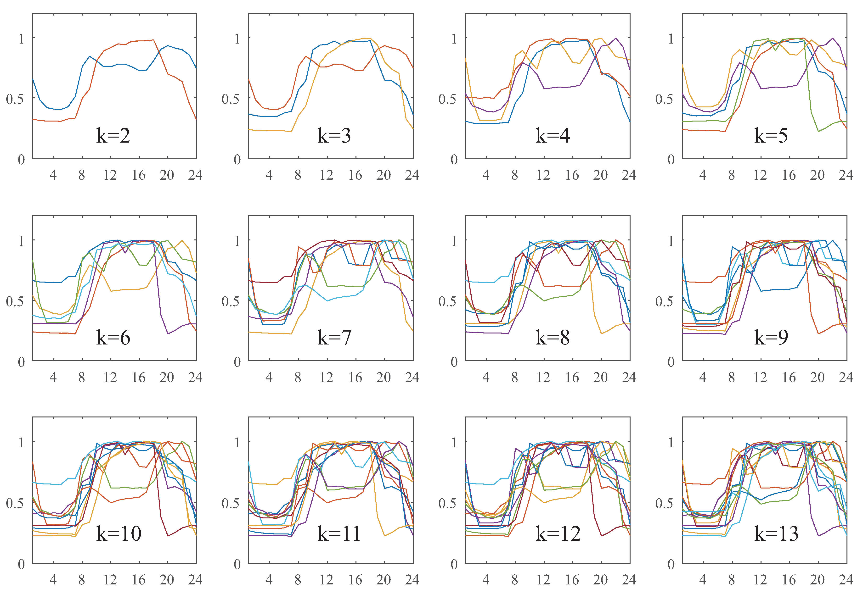
5.1. Basic Theory of k-Means Clustering

The k-means clustering is well known as the unsupervised learning method of machine learning. The algorithm classifies features to the number of k cluster from a data set by two steps. The first step is data assignment. All data point is assigned to cluster from set C as follows:

$$\underset{c_i\in C}{argmin}dist{(c_i,x)}^2$$

(16)

where dist(·) is the distance between point x and each ith cluster centroid $c_i$. Here, distance is applied as standard L2 distance. The second step is an update of the centroid. The new centroid position is calculated by assigned individuals $x_i$ of cluster $S_i$.

$$c_i^{(t+1)}=\frac{1}{|S_i^{\left(t\right)}|}\sum _{x_i\in S_i^{\left(t\right)}}{x}_i$$

(17)

The algorithm iterates until it satisfies the end criteria (e.g., no update centroid, no move $x_i$ between clusters, etc.).

The load profiles of clustering are shown in Figure 12 and Figure 13, respectively. The horizontal axis shows time and the vertical axis shows p.u. value. As k increases, it can be confirmed that the load changes. It can be confirmed that obvious characteristics include two kinds of patterns with a heavy load in the daytime, and peak load in the morning and the evening in the commercial area.

On the other hand, it can be confirmed that in the residential area, the load consumption shape is similar, but the width of max-min is different. In other words, it is difficult to judge how much load pattern can be extracted sufficiently to complement the load characteristics.

5.2. An Approach of Determining the Number of k Clusters

In many cases, data science cannot classify data unless it artificially adjusts the data, or researchers need to grasp the characteristics of the data beforehand. Here, even if clustering is used, since the number of k holds the key to the performance and suitability of clustering, the elbow method [36] is generally used to decide k number. This method judges the number of clusters’ appropriateness by a change of the sum of the squared errors ($SSE$) with cluster centroid and each point. However, as shown in Figure 14, the slope changes smoothly; it is not easy to specify a single point or an optimal point from the figure by applying the elbow method.

In addition, when it is precisely possible to group (e.g., even or odd number of groups are clear), the value of $SSE$ decreases as the number of clusters increases, however, the performance will show clear differences between the even and odd. Namely, it is not always number of cluster $k+1$ shows better performance for clustering than k. In order to ascertain such characteristics, it is possible to confirm the increment and decrement of SSE in the cluster center and cluster intervals by differentiating the sum of the squared errors ($DSSE$), thus making it possible to select the number of clusters more reliably.

The definition of $DSSE$ is determined as

$$DSSE=\frac{SSE(k+1)-SSE\left(k\right)}{N_{k+1}-N_k}$$

(18)

where $SSE\left(k\right)$ is $SSE$ of cluster number k, and $N_k$ is number of clusters. An applied $DSSE$ function value is shown in Figure 15. When the value of k is decided such that the change is small, the following formula can be applied.

$$DSSE\left(k_{n+1}\right)-DSSE\left(k_n\right)\le \left|ϵ\right|$$

(19)

In addition to this $DSSE$ value, the purpose is to decide on proper k from Equation (19). To determine the value of k from the $DSSE$, three points must be noted as listed below.

• $SSE$ is sufficiently small and SSE changes are also small, even if the value of k is increased.
• $DSSE$ value is not positive.
• Select valley point of $DSSE$.

Therefore, in the commercial area, k number was chosen to be 9, as shown Figure 15a. In the residential area, $k=9$ was chosen as shown in Figure 15b. Likewise, PV load was divided into 10 types and it was used for power distribution system analysis.

6. Simulation Results

Multiple simulations evaluated the performance of a smart inverter. Here, it first evaluates the cause of three-phase imbalance and its evaluation in a single time step statically. The PV connected phase is randomly selected, and the output thereafter is also chosen from the clustering profile so that unbalanced states are mixed in a complicated manner. This situation makes the three-phase imbalance more severe, and further responds transiently, making the system unstable. Then, it provides a case study on voltage compensation using the smart inverters with a battery:

• Active power regulation by battery (Volt-Watt control).
• Operation planning for reactive power control (Volt-Var control).
• Active and reactive power control for voltage unbalance compensation.

Note that the optimization of tap positions such as OLTC and step voltage regulator (SVR) is not considered this paper. For the performance evaluation of smart inverter, tap control is omitted.

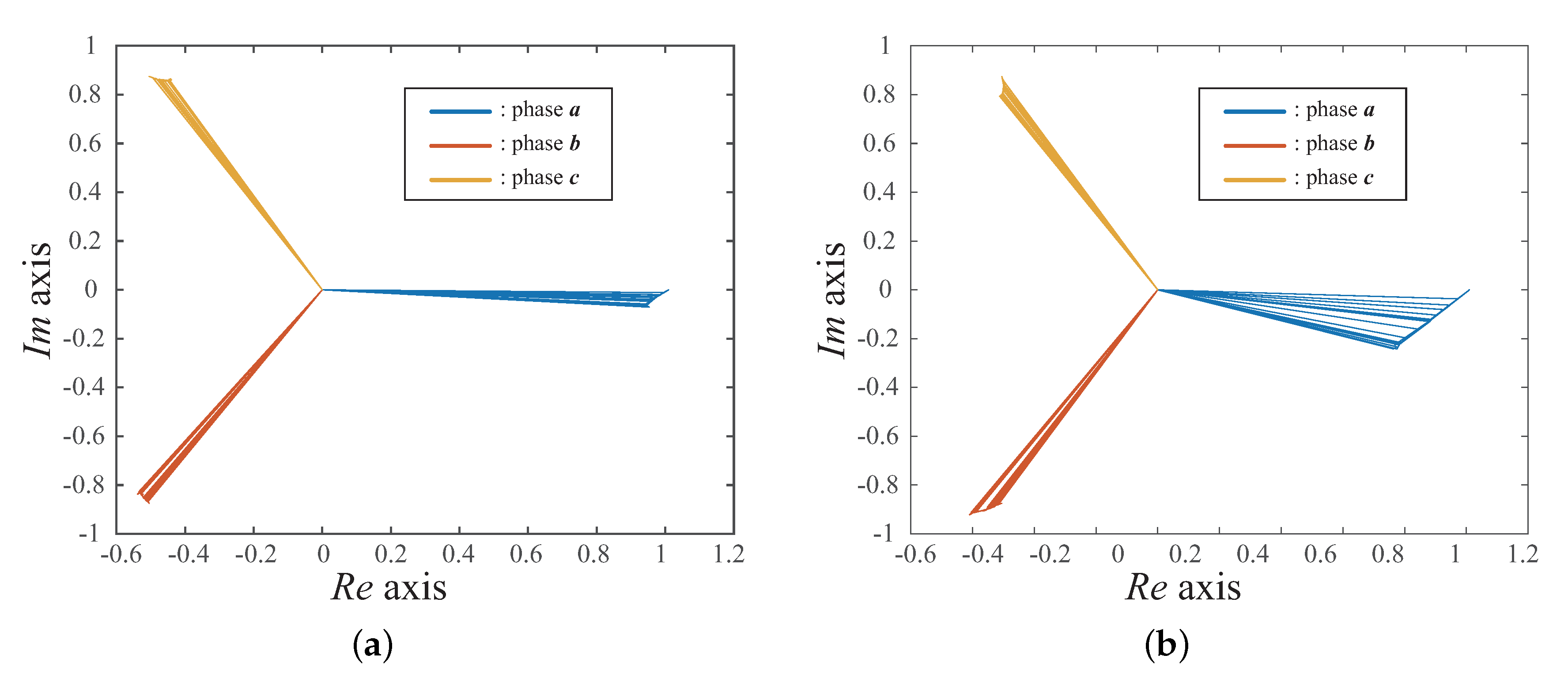
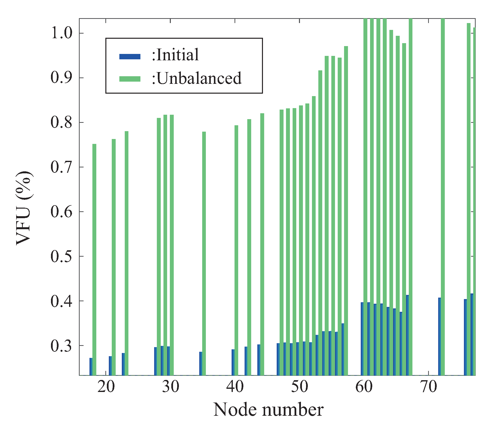
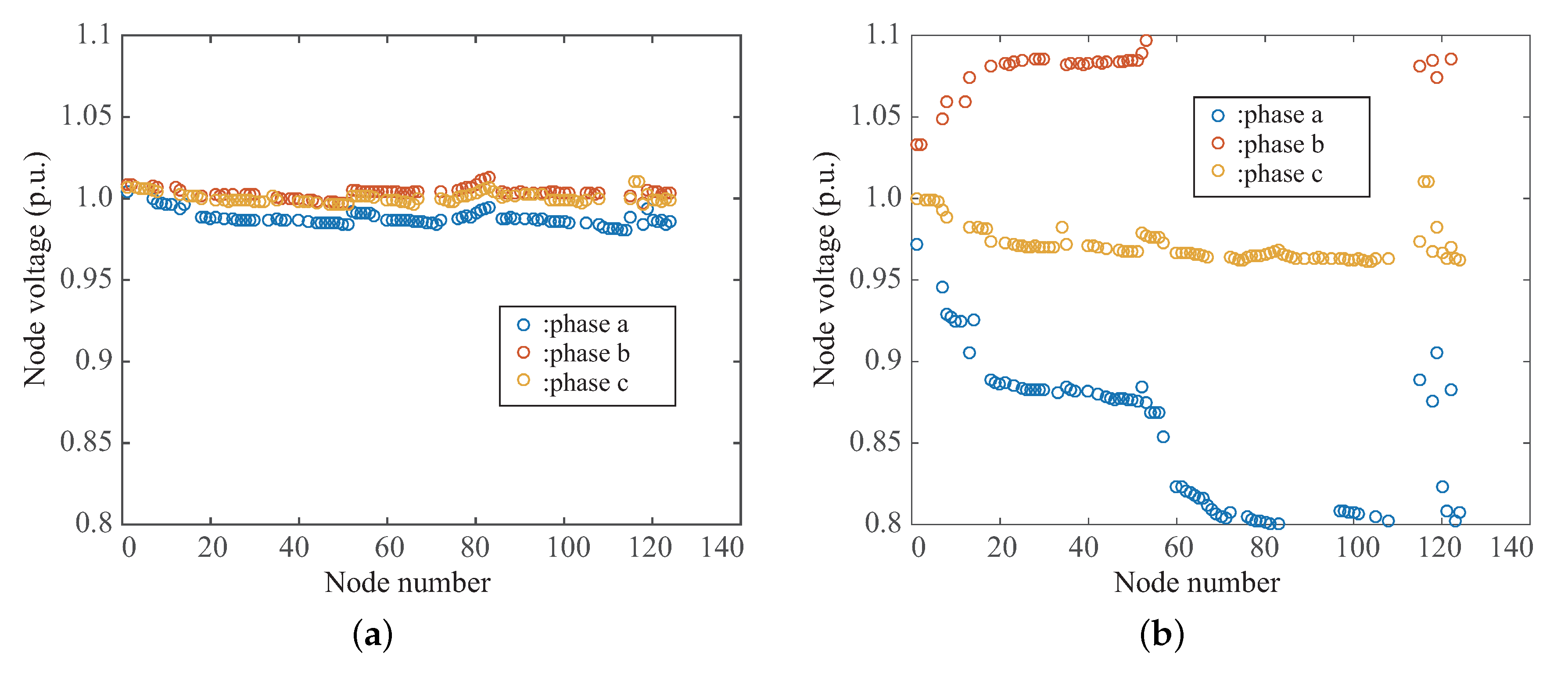
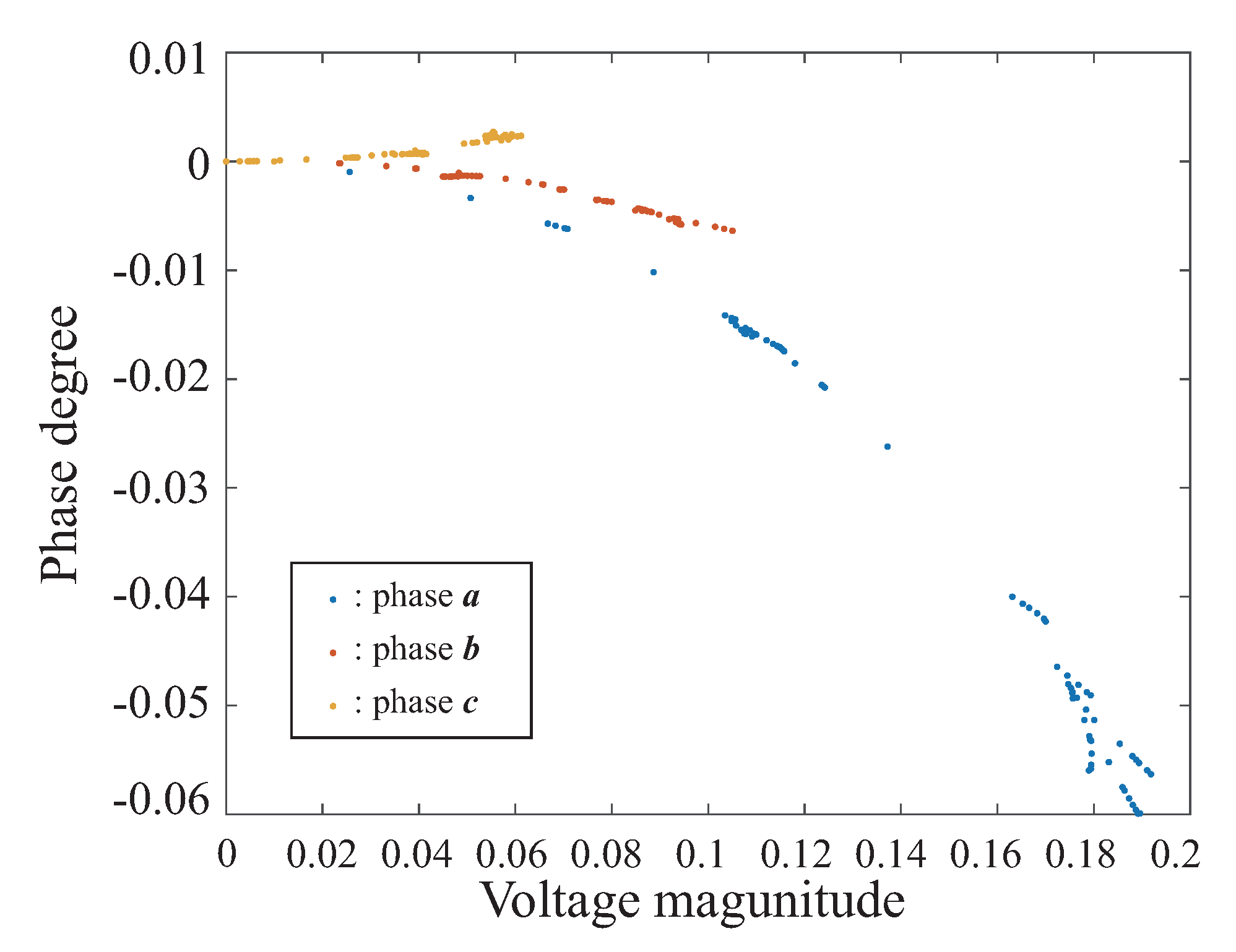
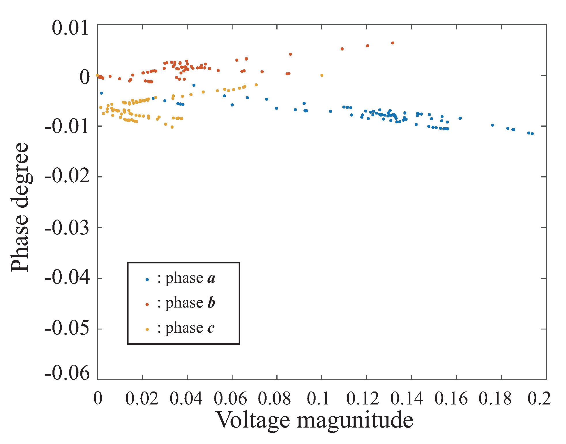
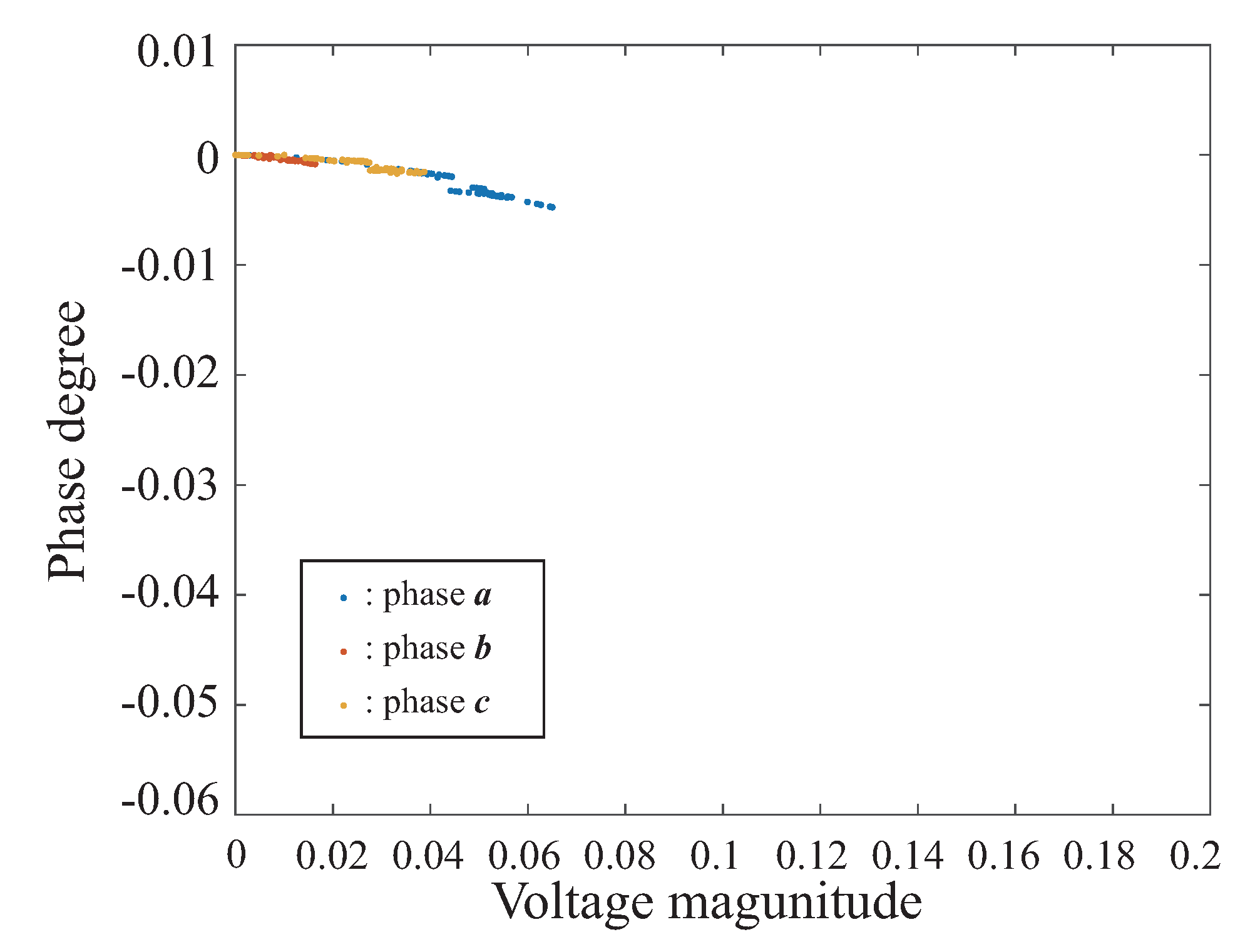
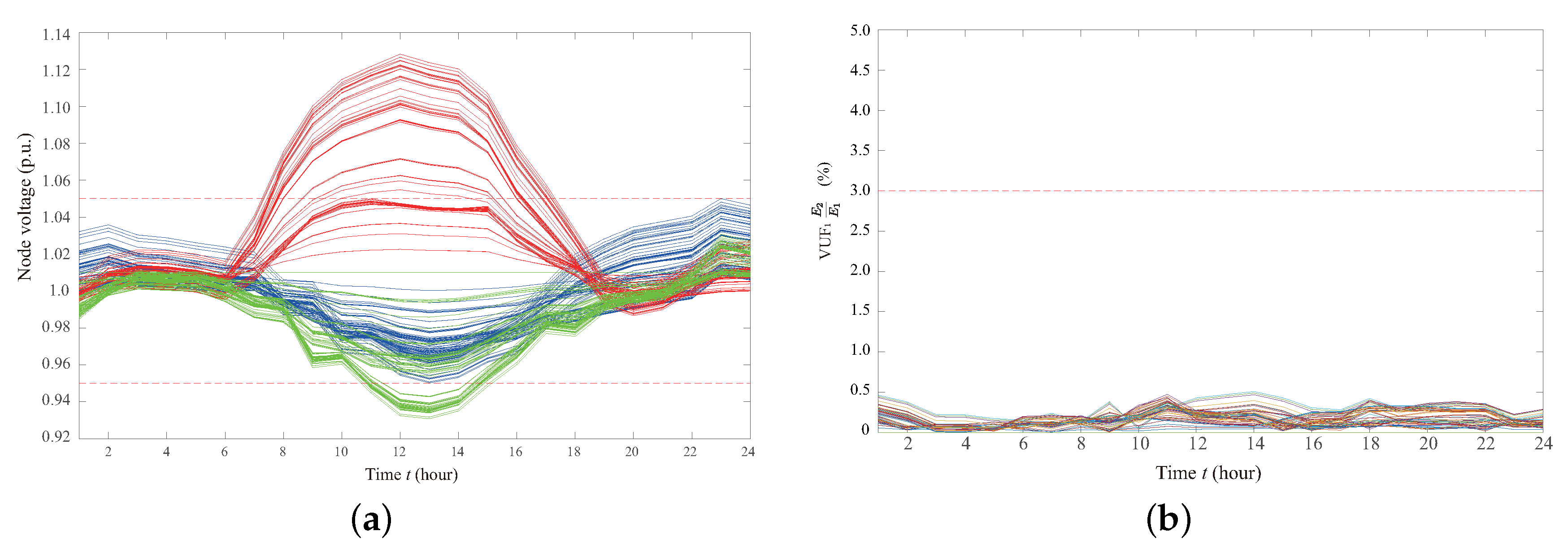
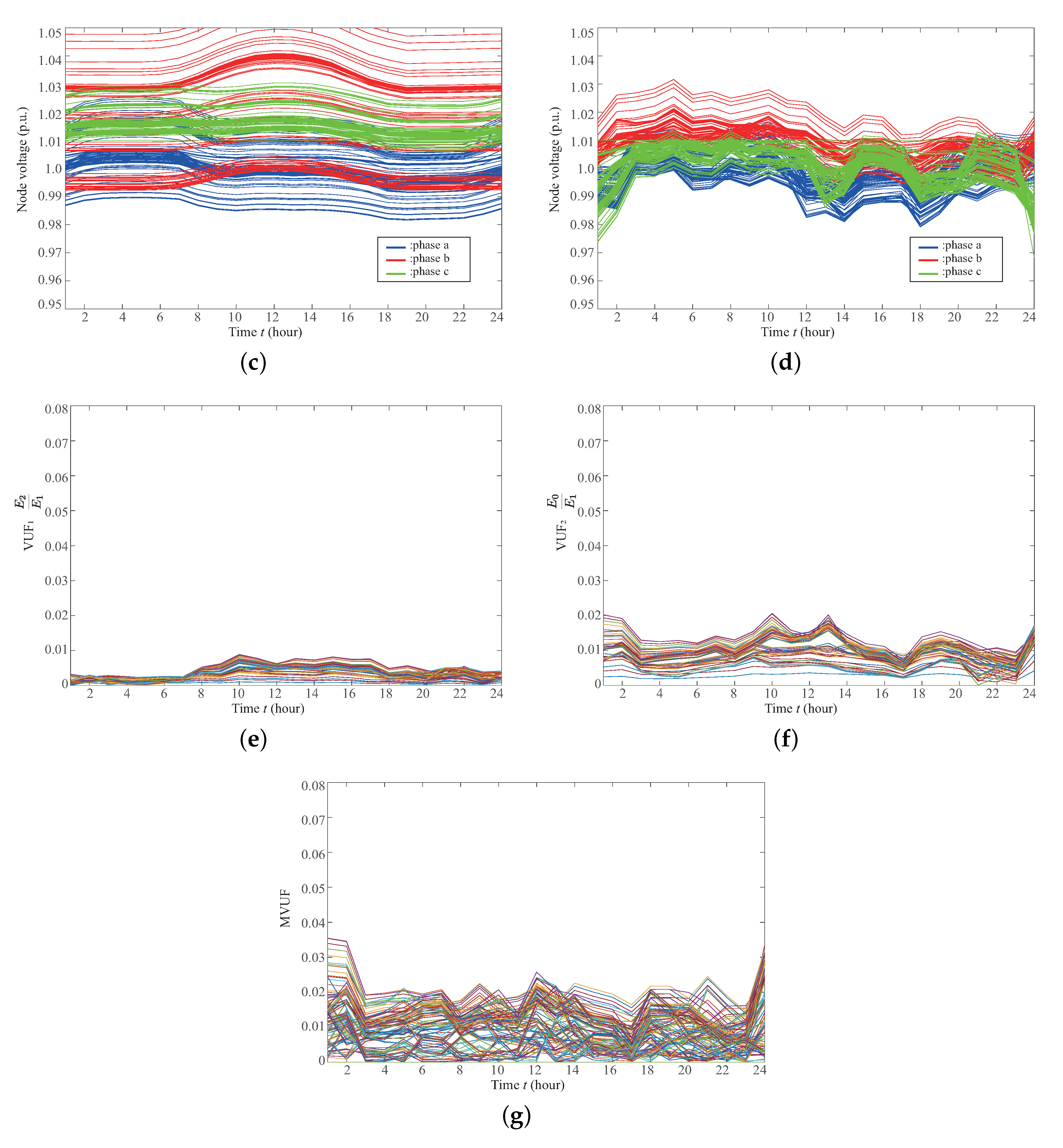
6.1. Assessment for Voltage Unbalance and Unbalance Compensation

There is a load imbalance due to the main cause of the three-phase imbalance. Furthermore, when a large amount of RES is introduced, it causes an unpredictable imbalance. Figure 16a shows the unbalanced state in the initial state provided by the IEEE 123 bus test system [37]. The imbalance slightly occurs in the load and the inductance component of the line. In Figure 16b, the RES is connected to the phases b and c with a heavy load on the phase a. It is confirmed from this figure that both magnitude and phase are unbalanced. However, these amounts cannot be quantitatively evaluated. Thus, to evaluate unbalance, the $VUF$ is applied to three-phase voltage as shown Figure 17. In this way, $VUF$ shows unbalance, but the imbalance of the magnitude of the voltage cannot be assessed. To observe an imbalance of the voltage magnitude, the magnitude of the voltage in the initial state and the unbalanced state is shown in Figure 18a,b, respectively.

The $VUF$ and unbalanced voltage magnitude should be assessed at the same time. Therefore, the phase is assigned to the vertical axis and the magnitude of the voltage is assigned to the horizontal axis, which is shown in Figure 19. It can be judged how far it deviates from the reference with this expression. Figure 19 is pictured at heavy load condition with no RES penetration. There is a voltage drop due to the load and line impedance. The system injected 200% to a phase and 50% load of b phase from initial condition. The results for the case when some RESs are connected to system are shown in Figure 20. Figure 21 illustrates an improvement in both the imbalance between the phase and the magnitude of the voltage due the smart invert output. It can be confirmed that the magnitude and phase of the three-phase voltage are closed to $O(0,0)$ point. The $VUF$ of each state is summarized in

Table 1. Three-phase voltage unbalance assessment.

Conditions	$VUF$	Sum of $VUF$
Initial case	0.02	0.2231
Heavy load	0.05	0.5896
Including RES generation	0.02	0.2221
Compensated voltage (optimized)	less than 0.01	0.098

. From the above results, it can be expected that smart inverters will contribute to a three-phase voltage of unbalance compensation.

6.2. Case Study for Active and Reactive Power ($PQ$) Control

In order to assume uncertainty and realistic situation, the load is selected from representative clustered real load data. The load is roughly divided into both commercial and residential areas and randomly selected from the prepared clusters.

Table 2. Data selection of load and PV output from big data.

	Commercial	Residential	PV
All data size	14,976 (building, one day)	3045 (house, one day)	365 (day)
cluster number k	9	9	10
Phase a	max 45 $\times N_{k,c}$ (kW)	max 30 $\times N_{k,r}$ (kW)	max 40 $\times N_{k,pv}$ (kW)
Phase b	30 $\times N_{k,c}$ (kW)	max 20 $\times N_{k,r}$ (kW)	max 60 $\times N_{k,pv}$ (kW)
Phase c	20 $\times N_{k,c}$ (kW)	max 20 $\times N_{k,r}$ (kW)	max 60 $\times N_{k,pv}$ (kW)

presents unbalanced introduction rates of load and PV power based on the c phase of the randomly selected load profile. In Table 2, $N_{k,c}$, $N_{k,r}$, and $N_{k,pv}$ are data type extracted by $k-$mean clustering.

In case of even minimized $VUF$ value (less than 1%), voltage unbalance, especially, voltage magnitude unbalance is still observed as shown Figure 22. In the worst case scenario, in worst it should be noted that even if the voltage deviates from the upper and lower statutory range, it is detected as an almost equilibrium state. Therefore, this paper proposes to define normal $VUF$ as $VU{F}_1$ and minimize $VU{F}_2=E_0/E_1$ and $MVUF$ (see Equation (1)) simultaneously for proper unbalance detection. In the following case study, the proposed voltage imbalance compensation method by P (volt-watt) and Q (volt-var) control using mixed $VUF$ indices is verified by numerical simulation.

6.2.1. Active Power (P) Control for Voltage Unbalance

A battery storage system can improve a three-phase imbalance by absorbing the surplus of negawatt trading. The constraint is mainly regarding the storage battery and the inverter restriction, but voltage modification by reactive power injection of an inverter is not performed in this case. Adjusting the power imbalance with active power P is synonymous with controlling current flow. The comparative analysis of the test results obtained from the proposed method regarding active power control are summarized in

Table 3. Simulation result of each case.

		P			Q			$\mathbf{PQ}$ (Proposed)
		only${\mathit{VUF}}_{\mathbf{1}}$	Proposed		only${\mathit{VUF}}_{\mathbf{1}}$	Proposed		only${\mathit{VUF}}_{\mathbf{1}}$	Proposed
$VU{F}_1$	max $VU{F}_1$	8.80(%)	2.51 (%)		4.90 (%)	1.65 (%)		0.87 (%)	0.89 (%)
	Sum of $VU{F}_1$	16.24	6.03		14.24	7.67		3.93	5.00
	max ave. $VU{F}_1$	2.61 (%)	0.80 (%)		1.68 (%)	0.48 (%)		0.30 (%)	0.30 (%)
		(12:00)	(16:00)		(10:00)	(14:00)		(12:00)	(10:00)
	ave. $VU{F}_1$	0.55 (%)	0.20 (%)		0.48 (%)	0.26(%)		0.13 (%)	0.17 (%)
$VU{F}_2$	max $VU{F}_2$	28.11 (%)	7.57 (%)		6.69 (%)	3.82 (%)		2.30 (%)	2.07 (%)
	Sum of $VU{F}_2$	47.76	22.51		19.70	9.65		14.90	14.02
	max ave. $VU{F}_2$	8.64 (%)	2.51 (%)		1.88 (%)	1.05 (%)		0.74 (%)	0.74 (%)
		(12:00)	(16:00)		(9:00)	(14:00)		(14:00)	(24:00)
	ave. $VU{F}_2$	1.60 (%)	0.76 (%)		0.66 (%)	0.32 (%)		0.50 (%)	0.47 (%)
$MVUF$	max $MVUF$	37.43(%)	9.10 (%)		14.68 (%)	5.64 (%)		3.76 (%)	3.55 (%)
	Sum of $MVUF$	89.44	45.91		44.4	35.20		30.70	29.62
	max ave. $MVUF$	15.24 (%)	3.89 (%)		5.83 (%)	2.55 (%)		1.73 (%)	1.78 (%)
		(12:00)	(16:00)		(10:00)	(19:00)		(8:00)	(24:00)
	ave. $MVUF$	3.01 (%)	1.54 (%)		1.49 (%)	1.18(%)		1.03 (%)	1.00 (%)

. In the comparison method, it can be confirmed that there is a significant difference between the minimum value of $VU{F}_1$ and the minimum amount of $VU{F}_2$. The unbalance rates of $VU{F}_2$ and $MVUF$ are 28% and 37%, respectively, and it can recognize that the voltage is deviating from the allowable range considerably. On the other hand, it can be confirmed that each value in the proposed method has a smaller amount than the comparison method. Additionally, the reduction of $VU{F}_2$ and $MVUF$ are remarkable as seen from the proposed method, which shows the effectiveness of the proposed method. Although the average value of the unbalances in the proposed method is 3% or less, each unbalance rate shows the maximum value when the load demand starts to increase rapidly (16:00 hours). The reason is the inverter output does not satisfy to compensate with the fluctuation, and it helps to recognize that it is not realistic to perform all of the unbalance with only P control of the interfaced inverter.

6.2.2. Reactive Power (Q) Control for Voltage Unbalance

In this case, utilize the available space of the inverter capacity equipped with the PV panel as the reactive power supply resource. The volt/var control has been widely adopted in recent years for voltage control and has been evaluated as one function of smart inverters. To evaluate the unbalanced compensation capability, which is used only as a supply of reactive power. Namely, active power management is not applied in this case. This is the function as the conventional smart inverter and is a control for distributed control. When considering the phase and the magnitude, it is related to power quality indicators, such as the power factor. As can be seen from Table 3, it can be confirmed that each unbalance rate is less than half in Q control, as similarly with the case of only P control. However, it is confirmed that the maximum value of $VU{F}_2$ in the proposed method exceeds 3%, and it is slightly insufficient for entirely desirable unbalance compensation.

6.2.3. Active and Reactive Power ($PQ$) Control for Voltage Unbalance

In contrast to control of only active or reactive power, because the inverter can control both $PQ$ values individually, it is assumed that it a control method using storage battery and interfaced inverter in the last case. In Table 3, in which all the case results are summarized, it can be confirmed that the control for adjusting both $PQ$ has the best compensation capability. In addition, when $PQ$ is injected, the convergence performance of $f_1$ (Equation (10)) is improved as calculation time is reduced by around 20%. In this case, there are some parts ($VUF$, $MVUF$) where the conventional method shows smaller values than the proposed method as shown in Table 3, however, this is due to the unbalanced connection state between the load and the PV; and the proposed method has higher convergence rate.

Figure 23 and Figure 24 show the minimized simulation results of the conventional index and the proposed index in the proposed three-phase unbalance compensation with active and reactive powers by smart inverter. In both Figure 23 and Figure 24, (a) is the load profile in each phase, (b) is a total load of node units, (c) is the voltage profile at before control, (d) is the voltage profile after compensation, and $VU{F}_1$, $VU{F}_2$ and $MUVF$ are shown in (e), (f), and (g), respectively. In the load state of each node, the load state does not change significantly between Figure 23b and Figure 24b, but it can be confirmed that the initial voltage state in Figure 24c is a more serious condition than the voltage profile of Figure 23c. After control, the unbalance rate $VU{F}_1$ becomes smaller than 3%, and active, reactive power control can alleviate the unbalanced state. However, when controlling with $PQ$, the unbalanced state could be compensated only by the $VU{F}_1$ index, but in rare cases, the unbalanced state may not be resolved even if $VU{F}_1$ is less than 3%. On the other hand, in the proposed index, such a situation never appeared in 1000 trials. The active and reactive power control with three $VUF$ indexes ($VU{F}_1$, $VU{F}_2$, and $MVUF$) can compensate voltage imbalance without undetectable unbalanced conditions. Consequently, the calculation time for optimization is reduced by about 20% because the indices avoid the unnecessary searching point.

7. Conclusions

The conventional voltage imbalance index and the situation of the index not being able to properly detect the unbalanced state are presented in this paper in the context of a power distribution system by utilizing a smart inverter. A mathematical approach elucidated the undetectable unbalance state and revealed that this undetectable unbalanced state occurs when RES was interconnected to the system. Test results demonstrated that the unbalance indication is significantly improved to overcome undetectable unbalance states, showing the superior performance of the proposed method over the conventional symmetric method. To evaluate the proposed index and the imbalance compensation with the smart inverter, voltage control in three scenarios (with P only, Q only, and both P and Q) was assessed using $PQ$ injection. It was clarified that the proposed unbalanced index and the voltage compensation method by smart inverter are useful in the distribution system in which RES is connected in a complicated manner. Test results further demonstrated that it is very important to consider the voltage control from the load demand side perspective. Moreover, this paper also contributed to the field of big data analytics by using k-means clustering in order to reduce the large volume of data for effective analysis of a smart power distribution system.

References

1. Nour, A.M. Review on voltage-violation mitigation techniques of distribution networks with distributed rooftop PV systems. IET Gener. Transm. Distrib. 2020, 14, 349–361. [Google Scholar] [CrossRef]
2. Iioka, D.; Fujii, T.; Orihara, D.; Tanaka, T.; Harimoto, T.; Shimada, A.; Goto, T.; Kubuki, M. Voltage reduction due to reverse power flow in distribution feeder with photovoltaic system. Int. J. Electr. Power Energy Syst. 2019, 113, 411–418. [Google Scholar] [CrossRef]
3. El-Hawary, M.E. Definitions of Voltage Unbalance. IEEE Power Eng. Rev. 2001, 21, 49–51. [Google Scholar]
4. Zaheb, H.; Danish, M.S.S.; Senjyu, T.; Ahmadi, M.; Nazari, A.M.; Wali, M.; Khosravy, M.; Mandal, P. A Contemporary Novel Classification of Voltage Stability Indices. Appl. Sci. 2020, 10, 1639. [Google Scholar] [CrossRef] [Green Version]
5. Ziadi, Z.; Oshiro, M.; Senjyu, T.; Yona, A.; Urasaki, N.; Funabashi, T.; Kim, C. Optimal Voltage Control Using Inverters Interfaced With PV Systems Considering Forecast Error in a Distribution System. IEEE Trans. Sustain. Energy 2014, 5, 682–690. [Google Scholar] [CrossRef]
6. Dao, V.T.; Ishii, H.; Hayashi, Y. Optimal smart functions of large-scale PV inverters in distribution systems. In Proceedings of the 2017 IEEE Innovative Smart Grid Technologies-Asia (ISGT-Asia), Auckland, New Zealand, 4–7 December 2017; pp. 1–7. [Google Scholar]
7. Adewuyi, O.B.; Ahmadi, M.; Olaniyi, I.O.; Senjyu, T.; Olowu, T.O.; Mandal, P. Voltage Security-Constrained Optimal Generation Rescheduling for Available Transfer Capacity Enhancement in Deregulated Electricity Markets. Energies 2019, 12, 4371. [Google Scholar] [CrossRef] [Green Version]
8. Brown, R.E.; Pinkerton, R. Distribution Reliability Optimization Using Synthetic Feeders. Energies 2019, 12, 3510. [Google Scholar] [CrossRef] [Green Version]
9. Lee, H.J.; Yoon, K.H.; Shin, J.W.; Kim, J.C.; Cho, S.M. Optimal Parameters of Volt–Var Function in Smart Inverters for Improving System Performance. Energies 2020, 13, 2294. [Google Scholar] [CrossRef]
10. Arbab-Zavar, B.; Palacios-Garcia, E.J.; Vasquez, J.C.; Guerrero, J.M. Smart Inverters for Microgrid Applications: A Review. Energies 2019, 12, 840. [Google Scholar] [CrossRef] [Green Version]
11. Srinivasarangan Rangarajan, S.; Sharma, J.; Sundarabalan, C.K. Novel Exertion of Intelligent Static Compensator Based Smart Inverters for Ancillary Services in a Distribution Utility Network-Review. Electronics 2020, 9, 662. [Google Scholar] [CrossRef] [Green Version]
12. Seguí-Chilet, S.; Gimeno-Sales, F.; Orts, S.; Garcerá, G.; Figueres, E.; Alcañiz, M.; Masot, R. Approach to unbalance power active compensation under linear load unbalances and fundamental voltage asymmetries. Int. J. Electr. Power Energy Syst. 2007, 29, 526–539. [Google Scholar] [CrossRef]
13. Rodríguez Paz, M.C.; Ferraz, R.G.; Bretas, A.S.; Leborgne, R.C. System unbalance and fault impedance effect on faulted distribution networks. Comput. Math. Appl. 2010, 60, 1105–1114. [Google Scholar] [CrossRef] [Green Version]
14. Jayatunga, U.; Perera, S.; Ciufo, P.; Agalgaonkar, A.P. Voltage Unbalance Emission Assessment in Interconnected Power Systems. IEEE Trans. Power Deliv. 2013, 28, 2383–2393. [Google Scholar] [CrossRef] [Green Version]
15. Bollen, M.; Zhang, L. Different methods for classification of three-phase unbalanced voltage dips due to faults. Electr. Power Syst. Res. 2003, 66, 59–69. [Google Scholar] [CrossRef]
16. Gnacinski, P. Windings Temperature and Loss of Life of an Induction Machine Under Voltage Unbalance Combined With Over or Undervoltages. IEEE Trans. Energy Convers. 2008, 23, 363–371. [Google Scholar] [CrossRef]
17. Kerekes, T.; Liserre, M.; Mastromauro, R.; Dell’Aquila, A. A Single-Phase Voltage-Controlled Grid-Connected Photovoltaic System With Power Quality Conditioner Functionality. IEEE Trans. Ind. Electron. 2009, 56, 4436–4444. [Google Scholar] [CrossRef]
18. Bonaldo, J.P.; Morales Paredes, H.K.; Pomilio, J.A. Control of Single-Phase Power Converters Connected to Low-Voltage Distorted Power Systems With Variable Compensation Objectives. IEEE Trans. Power Electron. 2016, 31, 2039–2052. [Google Scholar] [CrossRef] [Green Version]
19. Fan, L.; Miao, Z.; Domijan, A. Impact of unbalanced grid conditions on PV systems. In Proceedings of the IEEE PES General Meeting, Providence, RI, USA, 25–29 July 2010; pp. 1–6. [Google Scholar] [CrossRef]
20. Pou, J.; Boroyevich, D.; Pindado, R. Effects of imbalances and nonlinear loads on the voltage balance of a neutral-point-clamped inverter. IEEE Trans. Power Electron. 2005, 20, 123–131. [Google Scholar] [CrossRef]
21. Li, Y.; Vilathgamuwa, D.M.; Loh, P.C. Microgrid power quality enhancement using a three-phase four-wire grid-interfacing compensator. IEEE Trans. Ind. Appl. 2005, 41, 1707–1719. [Google Scholar] [CrossRef]
22. Li, Y.W.; Vilathgamuwa, D.M.; Loh, P.C. A grid-interfacing power quality compensator for three-phase three-wire microgrid applications. In Proceedings of the 2004 IEEE 35th Annual Power Electronics Specialists Conference (IEEE Cat. No.04CH37551), Aachen, Germany, 20–25 June 2004; Volume 3, pp. 2011–2017. [Google Scholar] [CrossRef]
23. George, S.; Agarwal, V. A DSP Based Optimal Algorithm for Shunt Active Filter Under Nonsinusoidal Supply and Unbalanced Load Conditions. IEEE Trans. Power Electron. 2007, 22, 593–601. [Google Scholar] [CrossRef]
24. Luo, A.; Peng, S.; Wu, C.; Wu, J.; Shuai, Z. Power Electronic Hybrid System for Load Balancing Compensation and Frequency-Selective Harmonic Suppression. IEEE Trans. Ind. Electron. 2012, 59, 723–732. [Google Scholar] [CrossRef]
25. Garcia-Cerrada, A.; Pinzon-Ardila, O.; Feliu-Batlle, V.; Roncero-Sanchez, P.; Garcia-Gonzalez, P. Application of a Repetitive Controller for a Three-Phase Active Power Filter. IEEE Trans. Power Electron. 2007, 22, 237–246. [Google Scholar] [CrossRef]
26. He, J.; Li, Y.W.; Munir, M.S. A Flexible Harmonic Control Approach Through Voltage-Controlled DG-Grid Interfacing Converters. IEEE Trans. Ind. Electron. 2012, 59, 444–455. [Google Scholar] [CrossRef]
27. Graovac, D.; Katic, V.; Rufer, A. Power Quality Problems Compensation With Universal Power Quality Conditioning System. IEEE Trans. Power Deliv. 2007, 22, 968–976. [Google Scholar] [CrossRef]
28. Lin, F.; Tan, K.; Lai, Y.; Luo, W. Intelligent PV Power System with Unbalanced Current Compensation Using CFNN-AMF. IEEE Trans. Power Electron. 2018. [Google Scholar] [CrossRef]
29. Yamane, K.; Orihara, D.; Iioka, D.; Aoto, Y.; Hashimoto, J.; Goda, T. Determination method of Volt-Var and Volt-Watt curve for smart inverters applying optimization of active/reactive power allocation for each inverter. Electr. Eng. Jpn. 2019, 209, 10–19. [Google Scholar] [CrossRef]
30. Smith, J.; Sunderman, W.; Dugan, R.; Seal, B. Smart inverter volt/var control functions for high penetration of PV on distribution systems. In Proceedings of the 2011 IEEE/PES Power Systems Conference and Exposition (PSCE), Phoenix, AZ, USA, 20–23 March 2011; pp. 1–6. [Google Scholar] [CrossRef]
31. Dao, V.T.; Ishii, H.; Takenobu, Y.; Yoshizawa, S.; Hayashi, Y. Home Energy Management Systems under Effects of Solar-Battery Smart Inverter Functions. IEEJ Trans. Electr. Electron. Eng. 2020, 15, 692–703. [Google Scholar] [CrossRef]
32. Jouanne, A.; Banerjee, B. Assessment of Voltage Unbalance. IEEE Trans. Power Deliv. 2001, 16, 782–790. [Google Scholar] [CrossRef]
33. Shigenobu, R.; Kinjo, M.; Mandal, P.; Howlader, A.M.; Senjyu, T. Optimal Operation Method for Distribution Systems Considering Distributed Generators Imparted with Reactive Power Incentive. Appl. Sci. 2018, 8, 1411. [Google Scholar] [CrossRef] [Green Version]
34. Building Characteristicsfor Residential Hourly Load Data. Available online: https://openei.org/doe-opendata/dataset/commercial-and-residential-hourly-load-profiles-for-all-tmy3-locations-in-the-united-states/resource/cd6704ba-3f53-4632-8d08-c9597842fde3 (accessed on 17 June 2020).
35. github/loads-clustering. Available online: https://github.com/gianlucahmd/loads_clustering (accessed on 17 June 2020).
36. Thorndike, R.L. Who belongs in the family? Psychometrika 1953, 18, 267–276. [Google Scholar] [CrossRef]
37. Kersting, W.H. Radial distribution test feeders. In Proceedings of the 2001 IEEE Power Engineering Society Winter Meeting. Conference Proceedings (Cat. No.01CH37194), Columbus, OH, USA, 28 January–1 February 2001; Volume 2, pp. 908–912. [Google Scholar]
Figure 1. A representation of voltage unbalance by complex plane.
Energies 13 04623 g001
Figure 2. A visualization of the symmetrical components in balanced three-phase conditions.
Energies 13 04623 g002
Figure 3. A graphical interpretation of V U F in the balanced case.
Energies 13 04623 g003
Figure 4. A visualization of the symmetrical components in unbalanced three-phase conditions.
Energies 13 04623 g004
Figure 5. A graphical interpretation of V U F in an unbalanced case.
Energies 13 04623 g005
Figure 6. An unbalanced condition but V U F 1 = 0 .
Energies 13 04623 g006
Figure 7. Graphical interpretation of V U F = 0 but an unbalanced case.
Energies 13 04623 g007
Figure 8. An example of undetectable unbalance points.
Energies 13 04623 g008
Figure 9. Undetectable unbalance points on the symmetrical component method: (a) 3D plot and (b) 2D plot.
Energies 13 04623 g009
Figure 10. Undetectable unbalance points on the d–q transformation: (a) 3D plot and (b) 2D plot.
Energies 13 04623 g010
Figure 11. Real load profiles in the commercial and residential areas: (a) commercial area, and (b) residential area.
Energies 13 04623 g011
Figure 12. A comparison for the decision maker of k cluster number (commercial area load profiles).
Energies 13 04623 g012
Figure 13. A comparison for the decision maker of k cluster number (residential area load profiles).
Energies 13 04623 g013
Figure 14. A comparison of SSE at commercial area and residential area.
Energies 13 04623 g014
Figure 15. DSSE value comparison: (a) commercial area and (b) residential area.
Energies 13 04623 g015
Figure 16. Phasor representation of three phases: (a) initial condition and (b) unbalanced condition.
Energies 13 04623 g016
Figure 17. Load unbalanced condition (load of phase a increased by 20%).
Energies 13 04623 g017
Figure 18. A comparison of M V U F : (a) initial state and (b) unbalanced state.
Energies 13 04623 g018
Figure 19. Deviation from base voltage (phasor: magnitude vs. degree) in the case of a heavy load.
Energies 13 04623 g019
Figure 20. A few phase unbalances in the case of penetrated RES.
Energies 13 04623 g020
Figure 21. Improved three-phase unbalanced voltage.
Energies 13 04623 g021
Figure 22. Minimized V U F but voltage imbalance remaining case: (a) voltage profiles and (b) V U F 1 values.
Energies 13 04623 g022
Figure 23. Simulation result of PQ control for unbalance compensation ( V U F 1 only): (a) load profile in each phase, (b) total load of node units, (c) voltage profile at before control, (d) voltage profile after compensation, (e) V U F 1 values, (f) V U F 2 values, and (g) M U V F values.
Energies 13 04623 g023aEnergies 13 04623 g023b
Figure 24. Simulation result of PQ control for unbalance compensation (proposed method): (a) load profile in each phase, (b) total load of node units, (c) voltage profile at before control, (d) voltage profile after compensation, (e) V U F 1 values, (f) V U F 2 values, and (g) M U V F values.
Energies 13 04623 g024aEnergies 13 04623 g024b