A Fast State Estimator for Integrated Electrical and Heating Networks


Abstract
1. Introduction
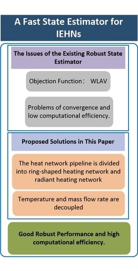
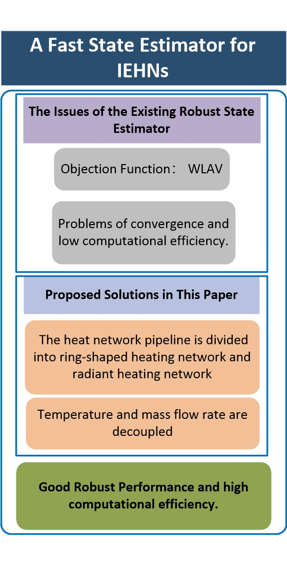
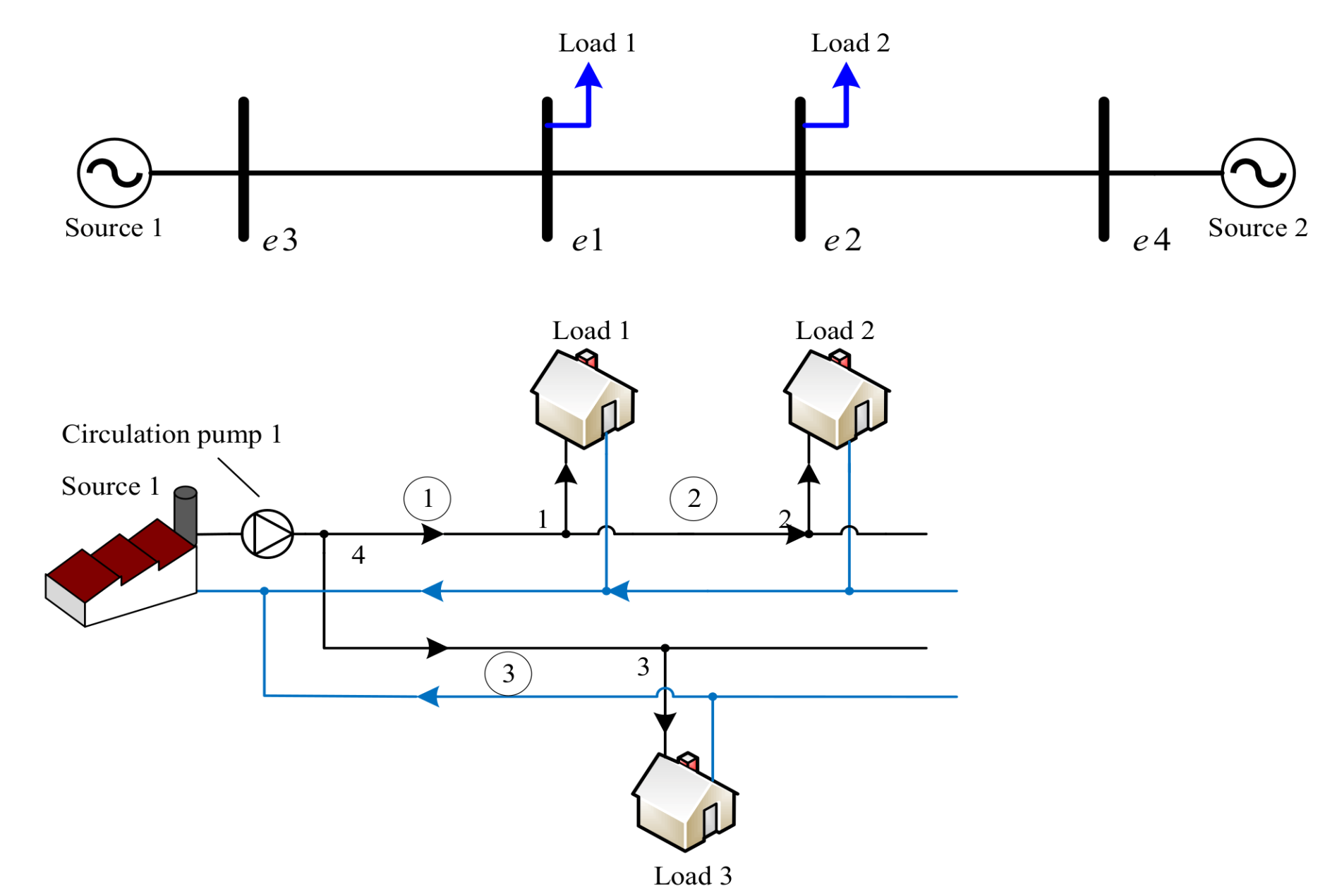
- Firstly, in the modeling and analysis of heating network, the heat network pipeline is divided into a ring-shaped heating network and radiant heating network. Under the assumption that the heating temperature and backwater temperature have little change in the actual heating network, the temperature and mass flow rate are decoupled to carry out in the state estimator of radiant heating network.
- In this paper, the state estimation of heating network is carried out from a distributed point of view. Boundary state constraints are set on the boundary of the ring-shaped heating network and radiant heating network. This method can improve the efficiency of IEHNs state estimation by simplifying the calculation scale of the ring-shaped heating network.
2. State Estimation Model for IEHNs
2.1. Objective Function
2.2. Constraints Equation
2.2.1. Power Constraints
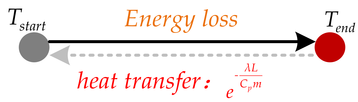
2.2.2. Thermal Constraints
2.2.3. Hydraulic Constraints
2.2.4. Coupling Component Constraints
3. Measurement Model for Heating Network
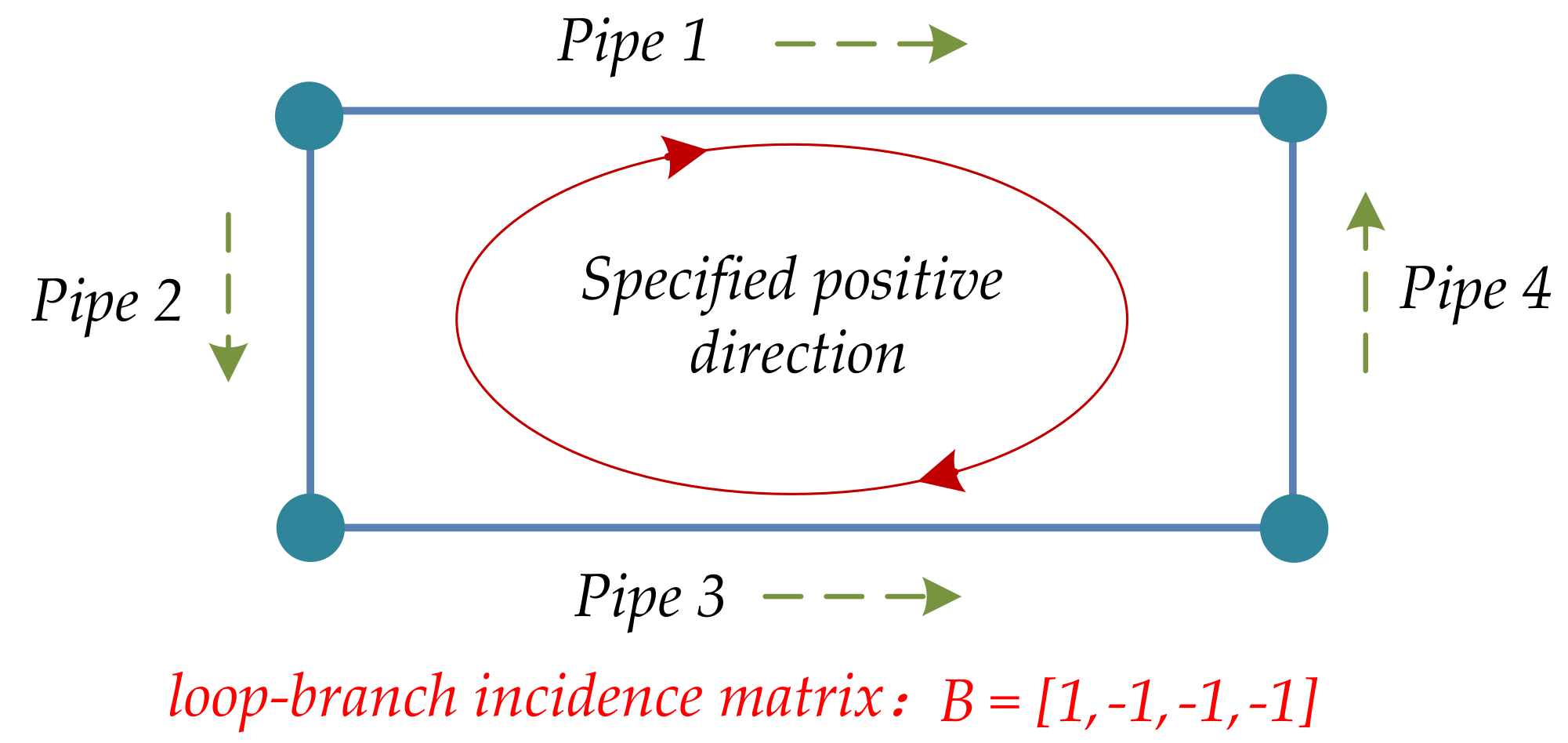
3.1. Ring-shaped Heating Network Measurement Models
3.2. Radiant Heating Network Measurement Model
4. Proposed Methodology
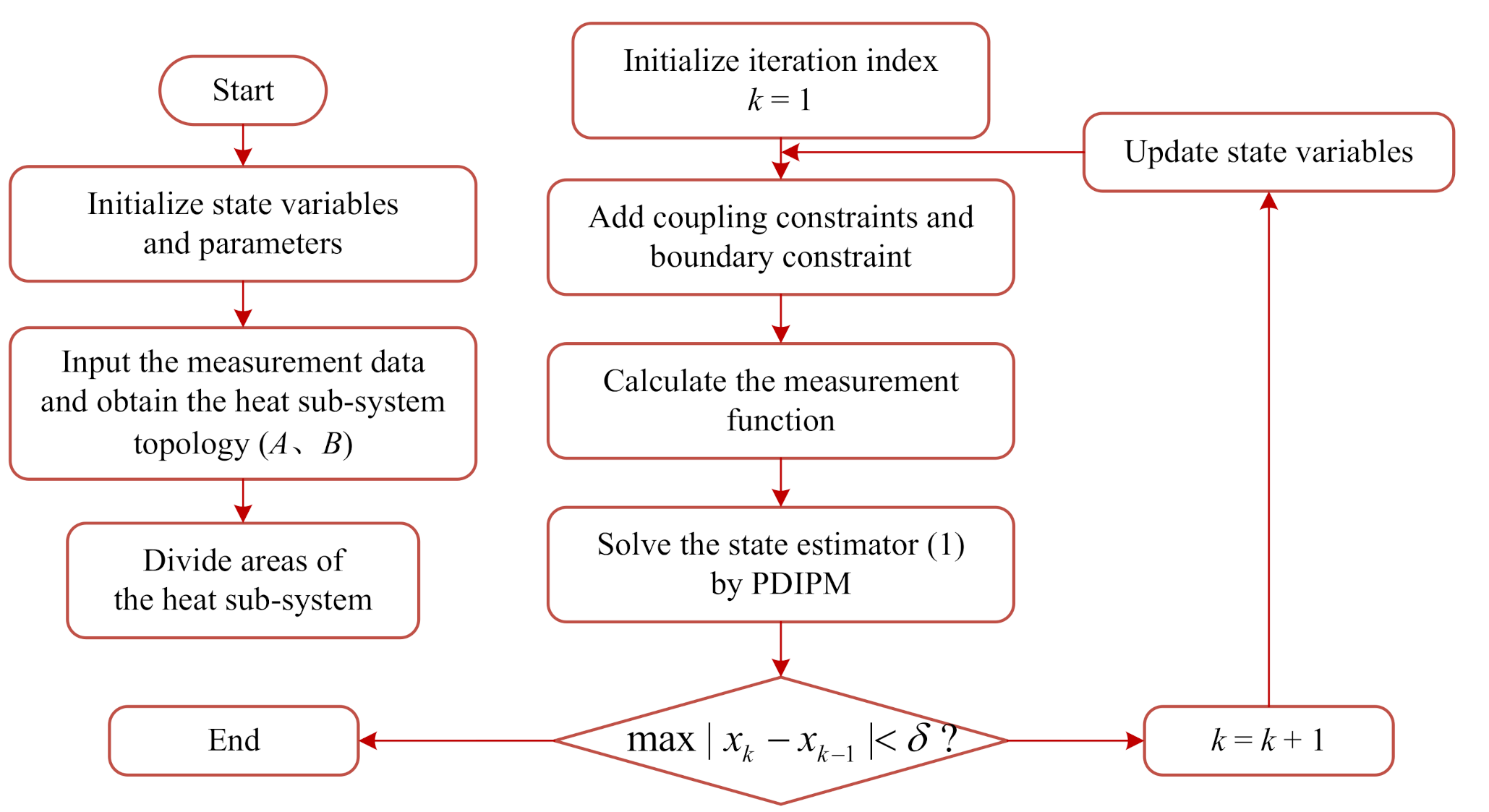
- Initializes the state variables and system parameters of the electricity subsystem and the heat subsystem.
- Input the real-time measurement data of the IEHN to determine the real-time topology of the heat subsystem.
- Based on the principle of the minimum number of nodes in the ring-shaped heating network, divide the heat subsystem and determine the boundary constraint.
- Input system coupling constraints and boundary state constraints.
- Calculate the measurement equation and . The measurement equation of the thermal model in the radiant partition is replaced by formula (16).
- Solve the state estimation model (1) by the primal-dual interior point method (PDIPM) [26].
- Judge whether the results satisfies the convergence condition .
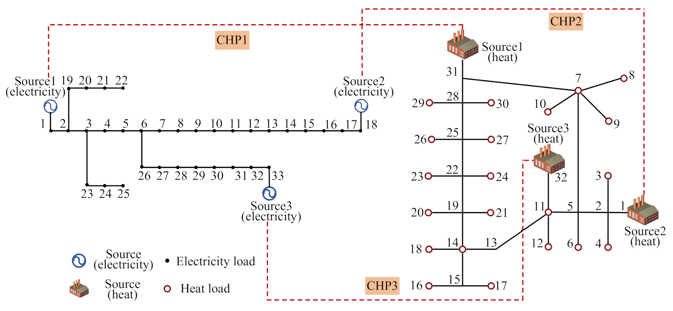
5. Simulation Study
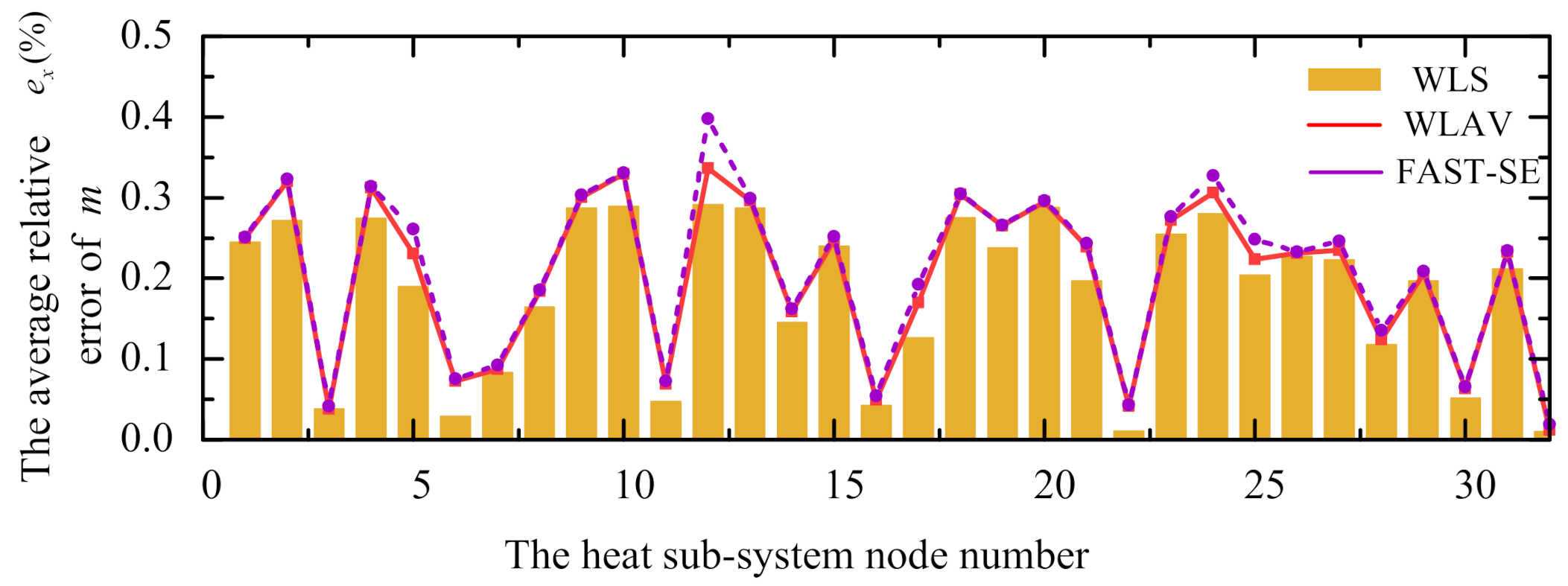
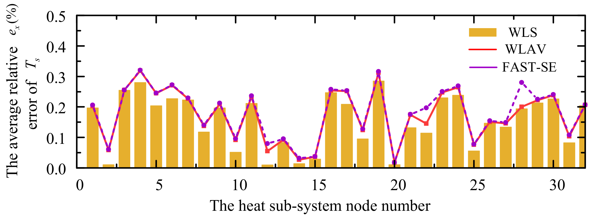
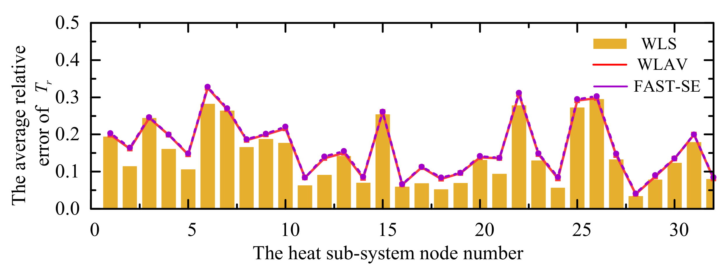
5.1. Accuracy of the State Estimator
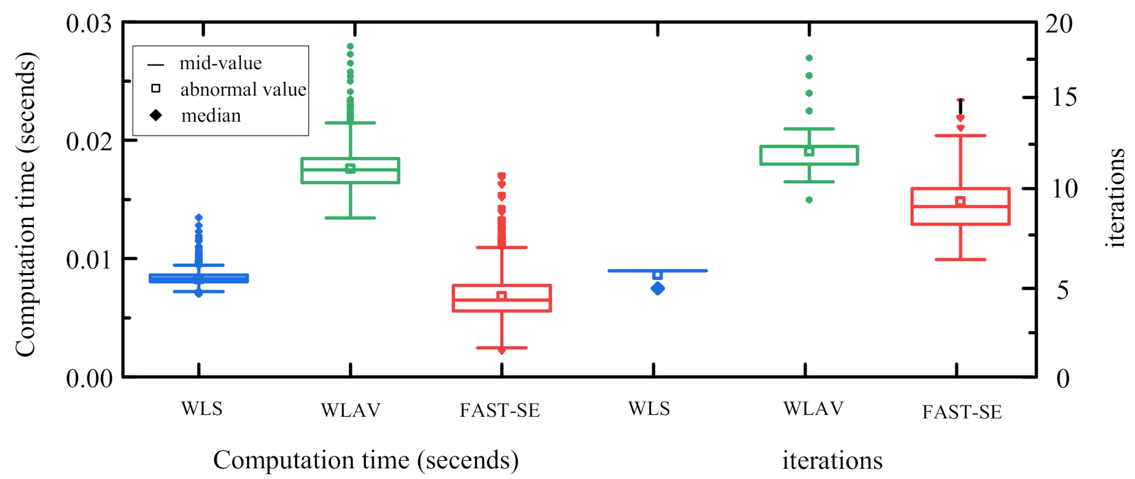
5.2. Computational Efficiency of the State Estimator
6. Conclusions
Author Contributions
Funding
Acknowledgments
Conflicts of Interest
Nomenclature
| A. Index | |
| IEHNs | integrated electrical and heating networks |
| SE | state estimation |
| WLS | weighted least square |
| WLAV | weighted least absolute value |
| set of the measurements in eps | |
| b. constant and coefficient | |
| node admittance matrix of electricity subsystem | |
| B | loop-branch incidence matrix |
| K | pipe resistance coefficient |
| node-branch incidence matrix | |
| coupling coefficient of CHP | |
| c. variables | |
| state variables of electricity subsystem | |
| state variables of heat subsystem | |
| measurement functions of electricity subsystem | |
| the ambient temperature | |
| measurement functions of heat subsystem | |
| measurements vector of electricity subsystem | |
| measurements vector of heat subsystem | |
| , | error variances columns of the measurements in the electricity subsystem and the heat subsystem |
| measurements of branch active power ij | |
| measurements of branch reactive power ij | |
| measurements of active injection power at node i | |
| measurements of reactive injection power at node i | |
| measurements of voltage magnitude at node i | |
| measurements of mass flow rates | |
| measurements of mass flow rates injected | |
| measurements of head losses | |
| measurements of heat power | |
| measurements of supply temperature | |
| measurements of return temperature | |
| , | the difference between supply / return temperature and the ambient temperature |
| outlet temperature before to mixing in the return network | |
| power generated by CHP | |
Appendix A. Parameters of Case Study 1
| Electricity Network |
| The base power is 1MVA and the base voltage is 11kV. |
| Voltage magnitude of the sources are: |V1,source| = 1.05 p.u., |V2,source| = 1.02 p.u. |
| Voltage angle of Source 2 at busbar 4 is: θ4 = 0°. |
| Active power of each load are: P1,load = P2,load = 0.15 MW. |
| Power factor of each load is: cosΦ = 0.95. |
| Impedance of each line is: Y = 0.09 + j0.1577p.u. |
| Heating Network |
| Φ1,load = Φ2,load = Φ3,load = 0.3 MW. |
| Ts1,source = 100 °C, To1,load = To2,load = To3,load = 50 °C. |
| Ambient temperature is: Ta = 10 °C. |
| The parameters of each pipe are: D = 0.15 m, ε = 1.25 × 10⁻³ m, λ = 0.2 W/mK, L = 400 m. |
| Water density is: ρ = 958.4 kg/m3. Cp = 4182 J/(kg·K)) = 4.182 × 10⁻³ MJ/(kg·K)). |
References
- Huang, A.Q.; Crow, M.L.; Heydt, G.T.; Zheng, J.P.; Dale, S.J. The Future Renewable Electric Energy Delivery and Management (FREEDM) System: The Energy Internet. Proc. IEEE 2011, 99, 133–148. [Google Scholar] [CrossRef]
- Gu, W.; Wu, Z.; Bo, R.; Liu, W.; Zhou, G.; Chen, W.; Wu, Z. Modeling, planning and optimal energy management of combined cooling, heating and power microgrid: A review. Int. J. Electr. Power Energy Syst. 2014, 54, 26–37. [Google Scholar] [CrossRef]
- Geidl, M.; Andersson, G. Optimal power flow of multiple energy carriers. IEEE Trans. Power Syst. 2007, 22, 145–155. [Google Scholar] [CrossRef]
- Jia, H.; Wang, D.; Xu, X.; Yu, X.D. Research on some key problems related to integrated energy systems. Autom. Electr. Power Syst. 2015, 39, 198–207. [Google Scholar]
- Wu, J.; Yan, J.; Jia, H.; Hatziargyriou, N.; Djilali, N.; Sun, H. Integrated Energy Systems. Appl. Energy 2016, 167, 155–157. [Google Scholar] [CrossRef]
- Chen, Q.; Hao, J.; Zhao, T. An alternative energy flow model for analysis and optimization of heat transfer systems. Int. J. Heat Mass Transf. 2017, 108, 712–720. [Google Scholar] [CrossRef]
- Liu, X.; Wu, J.; Jenkins, N.; Bagdanavicius, A. Combined analysis of electricity and heat networks. Appl. Energy 2016, 162, 1238–1250. [Google Scholar] [CrossRef]
- Zang, H.; Cheng, L.; Ding, T.; Cheung, K.W.; Wei, Z.; Sun, G. Day-ahead photovoltaic power forecasting approach based on deep convolutional neural networks and meta learning. Int. J. Electr. Power Energy Syst. 2020, 118, 105790. [Google Scholar] [CrossRef]
- Li, Z.; Wu, W.; Wang, J.; Zhang, B.; Zheng, T. Transmission-Constrained Unit Commitment Considering Combined Electricity and District Heating Networks. IEEE Trans. Sustain. Energy 2016, 7, 480–492. [Google Scholar] [CrossRef]
- Chen, S.; Wei, Z.; Sun, G.; Cheung, K.W.; Wang, D.; Zang, H. Adaptive Robust Day-Ahead Dispatch for Urban Energy Systems. IEEE Trans. Ind. Electron. 2019, 66, 1379–1390. [Google Scholar] [CrossRef]
- Li, R.; Wei, W.; Mei, S.; Hu, Q.; Wu, Q. Participation of an Energy Hub in Electricity and Heat Distribution Markets: An MPEC Approach. IEEE Trans. Smart Grid 2019, 10, 3641–3653. [Google Scholar] [CrossRef]
- Chen, S.; Wei, Z.; Sun, G.; Cheung, K.W.; Sun, Y. Multi-linear probabilistic energy flow analysis of integrated electrical and natural-gas systems. IEEE Trans. Power Syst. 2017, 32, 1970–1979. [Google Scholar] [CrossRef]
- Fang, T.; Lahdelma, R. State estimation of district heating network based on customer measurements. Appl. Therm. Eng. 2014, 73, 1211–1221. [Google Scholar] [CrossRef]
- Dong, J.; Guo, Q.; Sun, H.; Pan, Z. Research on state estimation for combined heat and power networks. In Proceedings of the IEEE Power and Energy Society General Meeting (PESGM), Boston, MA, USA, 17–21 July 2016. [Google Scholar]
- Sheng, T.; Guo, Q.; Sun, H.; Pan, Z.; Zhang, J. Two-stage State Estimation Approach for Combined Heat and Electric Networks Considering the Dynamic Property of Pipelines. Energy Procedia 2017, 142, 3014–3019. [Google Scholar] [CrossRef]
- Zhang, T.; Li, Z.; Wu, Q.; Zhou, X. Decentralized state estimation of combined heat and power systems using the asynchronous alternating direction method of multipliers. Appl. Energy 2019, 248, 600–613. [Google Scholar] [CrossRef]
- Zang, H.; Geng, M.; Xue, M.; Mao, X.; Huang, M.; Chen, S.; Wei, Z.; Sun, G. A Robust State Estimator for Integrated Electrical and Heating Networks. IEEE Access 2019, 7, 109990–110001. [Google Scholar] [CrossRef]
- Chen, Y.; Zheng, S.; Yang, N.; Lang, Y. Bilinear robust state estimation method for integrated electricity-heat energy systems. Electr. Power Autom. Equip. 2019, 39, 47–54. [Google Scholar]
- Sheng, T.; Yin, G.; Guo, Q.; Sun, H.; Pan, Z. A Hybrid State Estimation Approach for Integrated Heat and Electricity Networks Considering Time-scale Characteristics. J. Mod. Power Syst. Clean Energy 2020, 8, 636–645. [Google Scholar] [CrossRef]
- Zheng, W.; Li, Z.; Liang, X.; Zheng, J.; Wu, Q.H.; Hu, F. Decentralized State Estimation of Combined Heat and Power System Considering Communication Packet Loss. J. Mod. Power Syst. Clean Energy 2020, 8, 646–656. [Google Scholar] [CrossRef]
- Chen, Y.; Zheng, S.; Yang, N.; Yang, X.; Liu, K. Robust State Estimation of Electric-Gas Integrated Energy System Based on Weighted Least Absolute Value. Autom. Electr. Power Syst. 2019, 43, 1000–1026. [Google Scholar]
- Zheng, S.; Liu, J.; Chen, Y.; Qi, B. Bilinear Robust State Estimation Based on Weighted Least Absolute Value for Integrated Electricity-gas System. Power Syst. Technol. 2019, 43, 3733–3744. [Google Scholar]
- Gomez-Exposito, A.; Gomez-Quiles, C.; Jaen, A.D.L.V. Bilinear power system state estimation. IEEE Trans. Power Syst. 2012, 27, 493–501. [Google Scholar] [CrossRef]
- Gol, M.; Abur, A. LAV Based Robust State Estimation for Systems Measured by PMUs. IEEE Trans. Smart Grid 2014, 5, 1808–1814. [Google Scholar] [CrossRef]
- Sun, G.; Wang, W.; Wu, Y.; Hu, W.; Jing, J.; Wei, Z.; Zang, H.I. Fast Power Flow Calculation Method for Radiant Electric-Thermal Interconnected Integrated Energy System. Proc. Chin. Soc. Electr. Eng. 2020, 20, 436–443. [Google Scholar]
- Wei, H.; Sasaki, H.; Kubokawa, J.; Yokoyama, R. An interior point method for power system weighted nonlinear L-1 norm static state estimation. IEEE Trans. Power Syst. 1998, 13, 617–623. [Google Scholar] [CrossRef]


| Case | Algorithm | Power Network | Heating Network | ||||
|---|---|---|---|---|---|---|---|
| SM | SH | Ratio(%) | SM | SH | Ratio(%) | ||
| 1 | WLS | 0.9901 | 0.5425 | 54.79 | 0.9901 | 0.5127 | 51.78 |
| WLAV | 0.9901 | 0.5574 | 56.30 | 0.9898 | 0.5247 | 53.01 | |
| FAST-SE | 0.9901 | 0.5573 | 56.29 | 0.9900 | 0.5250 | 53.03 | |
| 2 | WLS | 0.9966 | 0.4439 | 44.54 | 0.9924 | 0.3538 | 35.65 |
| WLAV | 0.9966 | 0.5245 | 52.62 | 0.9924 | 0.3719 | 37.47 | |
| FAST-SE | 0.9966 | 0.5249 | 52.66 | 0.9924 | 0.3797 | 38.26 | |
| Case | Algorithm | Computational Time | Iterations |
|---|---|---|---|
| 1 | WLS | 0.0466 s | 4 |
| WLAV | 0.0652 s | 12 | |
| FAST-SE | 0.0173 s | 6 | |
| 2 | WLS | 0.0874 s | 5 |
| WLAV | 0.1822 s | 13 | |
| FAST-SE | 0.0693 s | 8 |
© 2020 by the authors. Licensee MDPI, Basel, Switzerland. This article is an open access article distributed under the terms and conditions of the Creative Commons Attribution (CC BY) license (http://creativecommons.org/licenses/by/4.0/).
Share and Cite
Wang, C.; Geng, M.; Xu, Q.; Zang, H. A Fast State Estimator for Integrated Electrical and Heating Networks. Energies 2020, 13, 4488. https://doi.org/10.3390/en13174488
Wang C, Geng M, Xu Q, Zang H. A Fast State Estimator for Integrated Electrical and Heating Networks. Energies. 2020; 13(17):4488. https://doi.org/10.3390/en13174488
Chicago/Turabian StyleWang, Chun, Minghao Geng, Qingshan Xu, and Haixiang Zang. 2020. "A Fast State Estimator for Integrated Electrical and Heating Networks" Energies 13, no. 17: 4488. https://doi.org/10.3390/en13174488
APA StyleWang, C., Geng, M., Xu, Q., & Zang, H. (2020). A Fast State Estimator for Integrated Electrical and Heating Networks. Energies, 13(17), 4488. https://doi.org/10.3390/en13174488