Mixed-Integer Programming Model for Transmission Network Expansion Planning with Battery Energy Storage Systems (BESS)


Abstract
1. Introduction
1.1. Background
1.2. Hypothesis and Aims
1.3. Contributions
- Include BESS in dynamic TEP problems with MIP. It is considered a joint optimization process to maximize the total benefit of the system through the construction of transmission lines and the installation of energy storage systems, taking into account the decrease in battery storage capacity and losses on the lines.
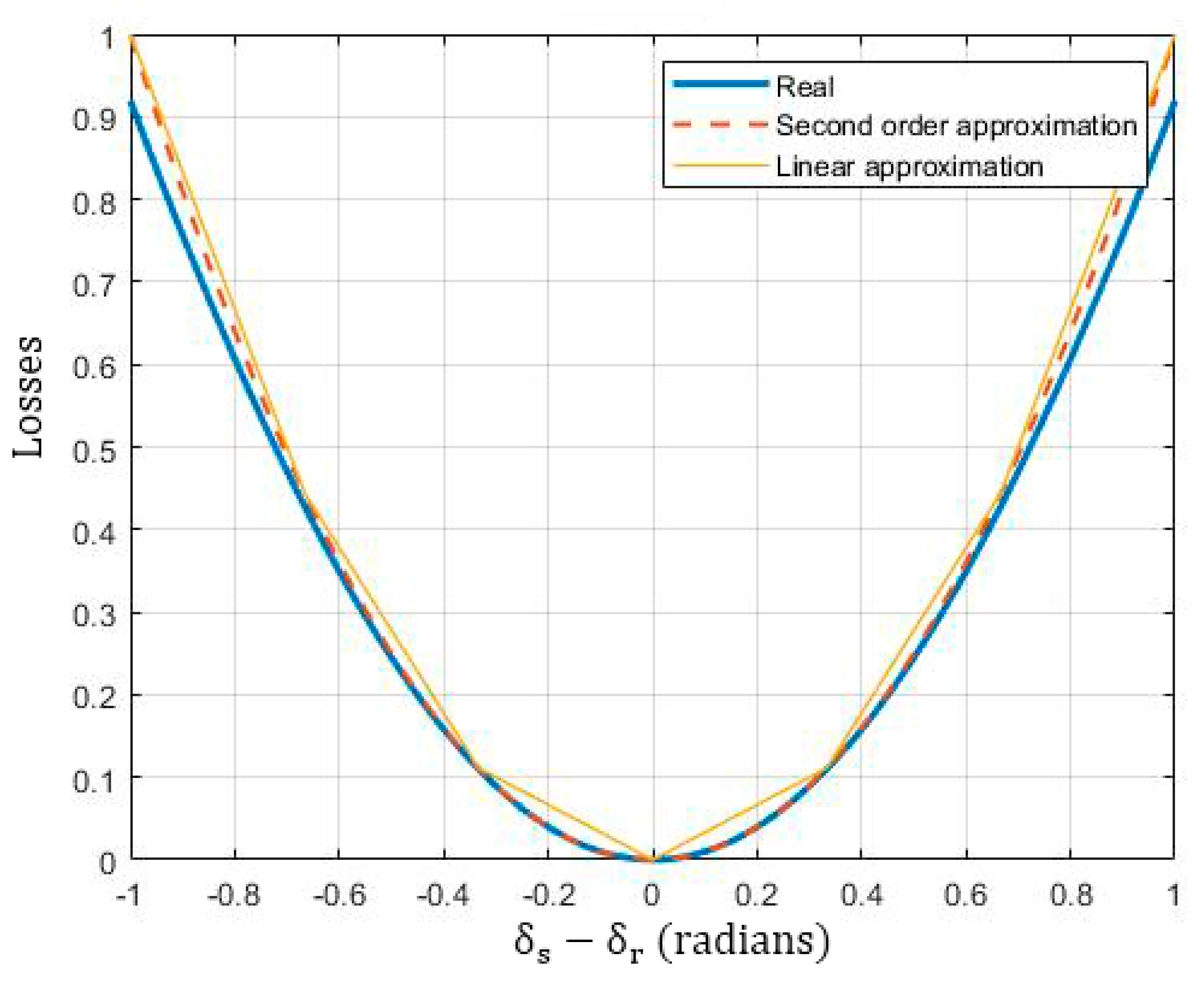
- Perform a sensitivity analysis to describe the relationship between the number of loss linearization blocks, execution times, and model accuracy.
- Validate the approaches made for power flows and losses in the network. Through the comparison of DC power flows of the MIP model with simulations for AC power flows in specialized software for power systems (i.e., Disigilent Powerfactory 15.7).
1.4. Article Organization
2. Literature Review
3. Methodology and Results
3.1. BESS Model
3.2. Power Flow Formulation
- Only active power flows exist.
- RL << XL.
- The voltages on all nodes are equal to 1 pu.
- The difference in the stress angles of the bars is very small.
3.3. Formulation of TEP with BESS
3.3.1. Objective Function
3.3.2. Constraints
3.4. Indices and Metrics
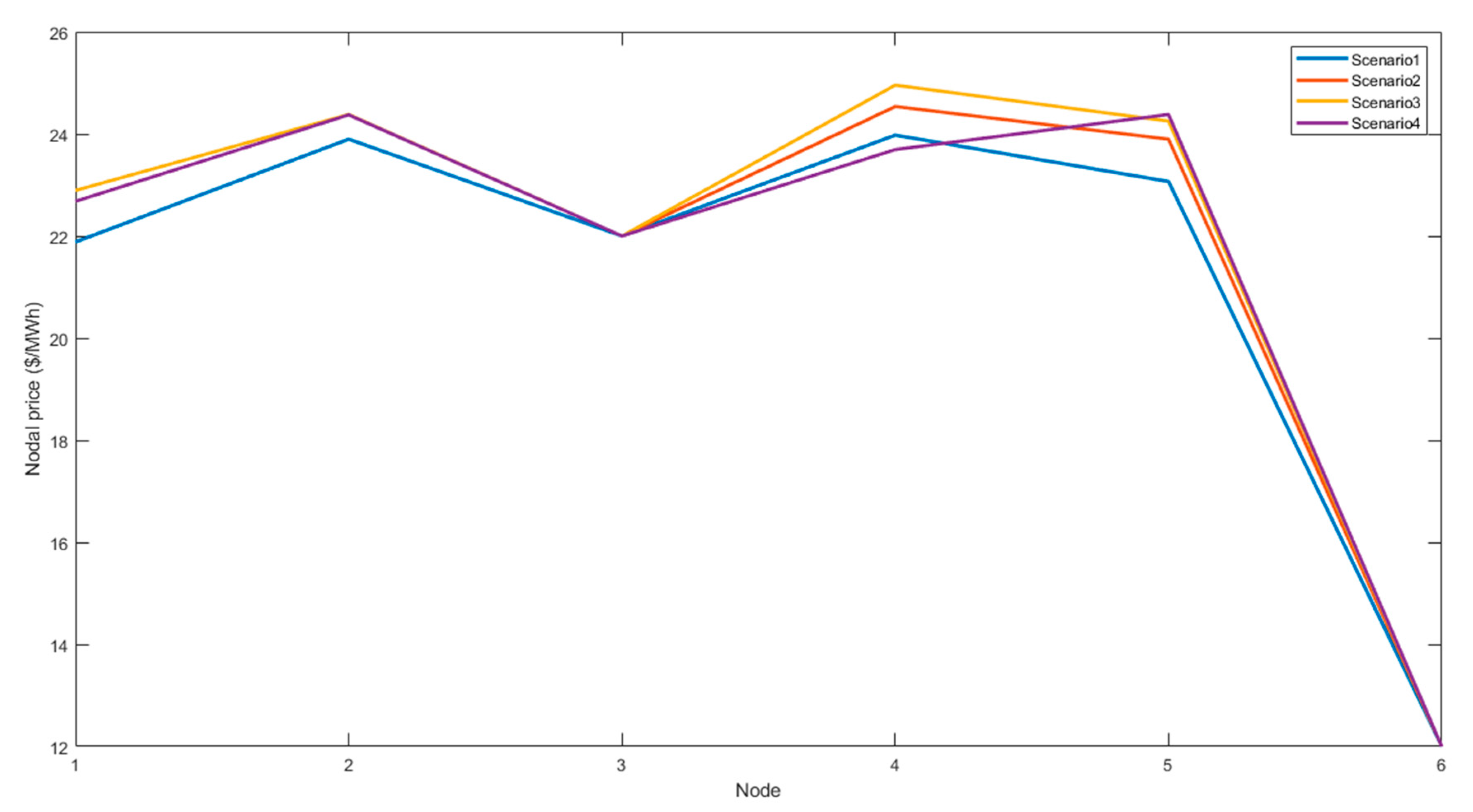
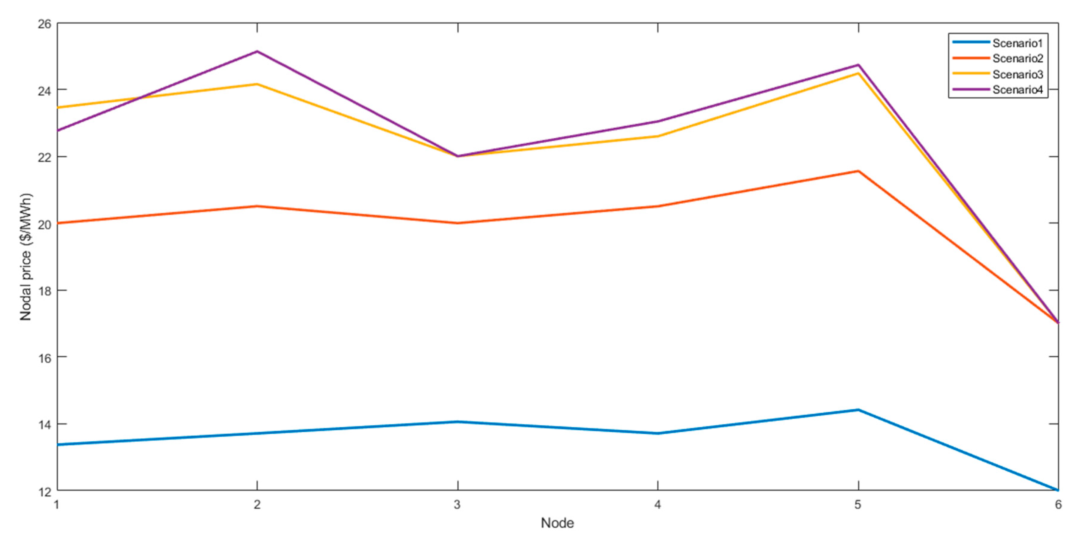
3.4.1. Nodal Prices
- Calculate the solution to the mixed-integer programming problem defined in Equations (18)–(36).
- Formulate a linear programming model, establishing binary variables and the optimal demand solution at each node as constants. The objective function for the linear programming model is presented in (37). The constraints are the same as those described in (19)–(36).
- Solve the linear programming model for each of the scenarios. The dual variables associated with the load balance equation are used as nodal prices.
3.4.2. Saturation Index
3.4.3. Congestion Index
3.4.4. Metrics
- μ1 Shows the changes in the aggregate social benefit of the general system in relation to investment costs.
- μ2 Describes the change in generation surpluses with respect to investment costs.
- Describes the change in generation and batteries surpluses with respect to investment costs.
- μ3 Describes the change in demand surpluses with respect to investment costs.
- μ4 Describes the change in marketer surpluses relative to investment costs. The marketer’s surpluses are equal to the subtraction of the total remuneration of the generators less the total payment for energy consumed from the demands.
3.5. Results
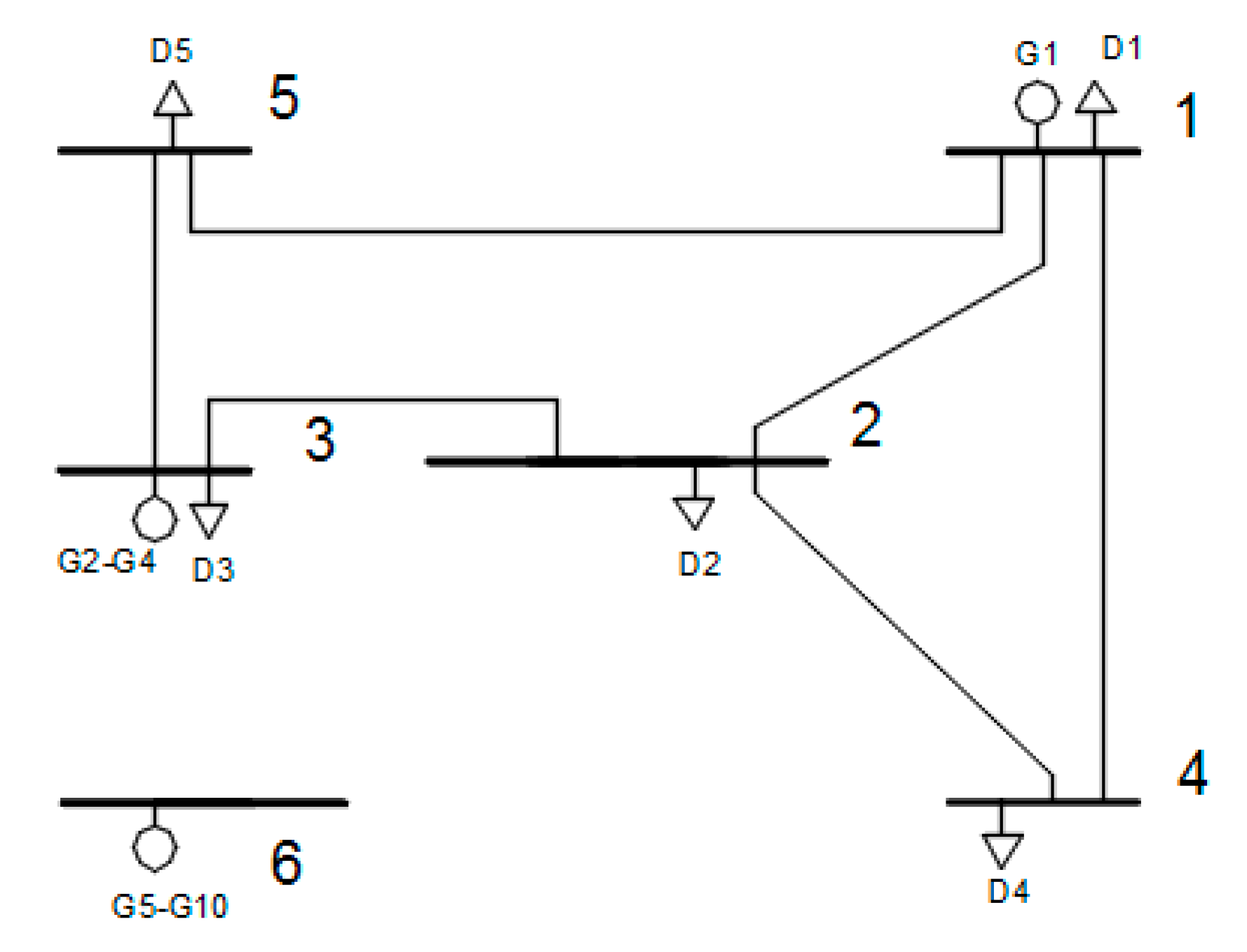
3.5.1. Garver 6 Node Test System
3.5.2. Case Study 1: Expansion with Lines
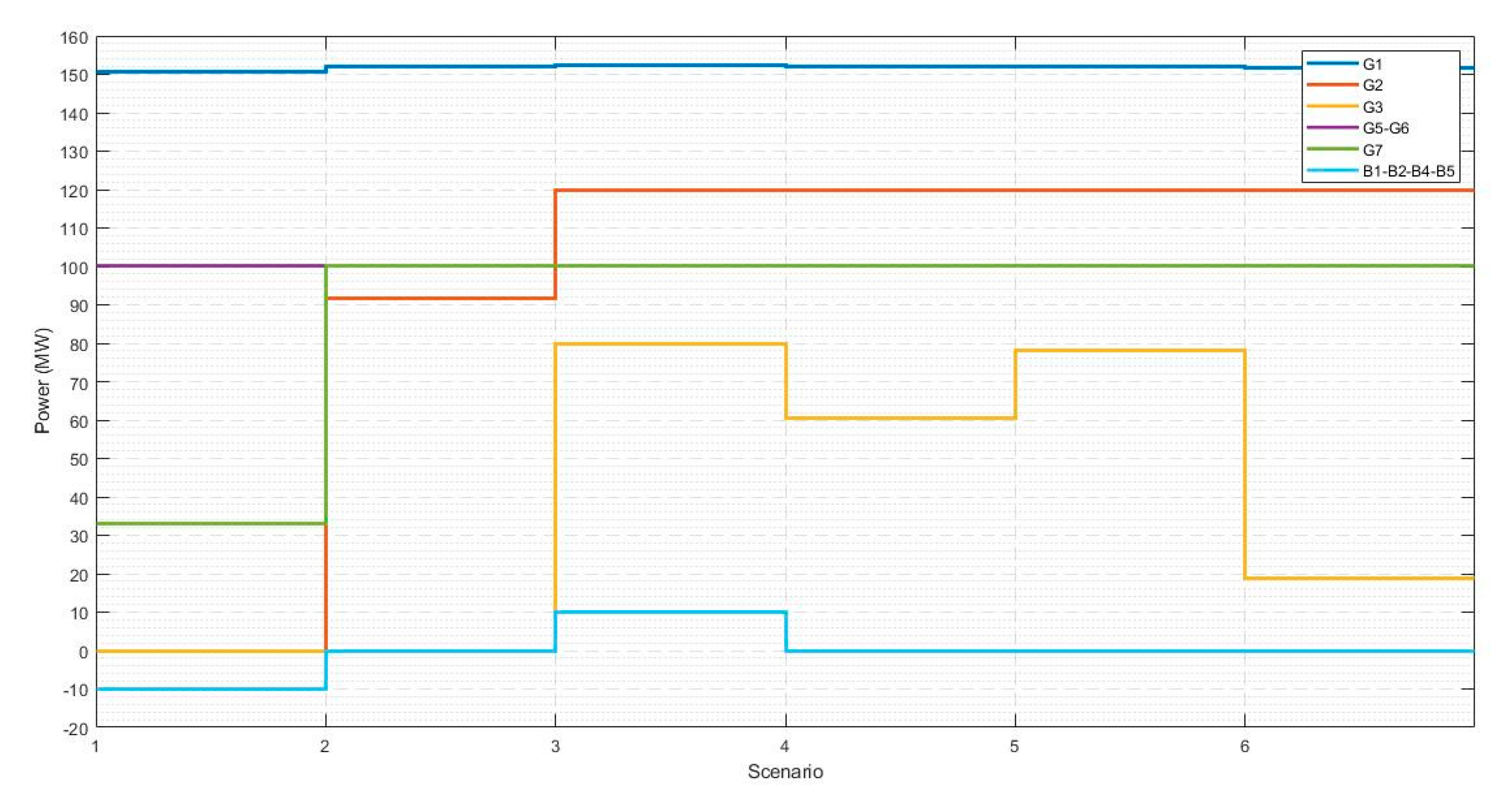
3.5.3. Case Study 2: Expansion with Lines and BESS
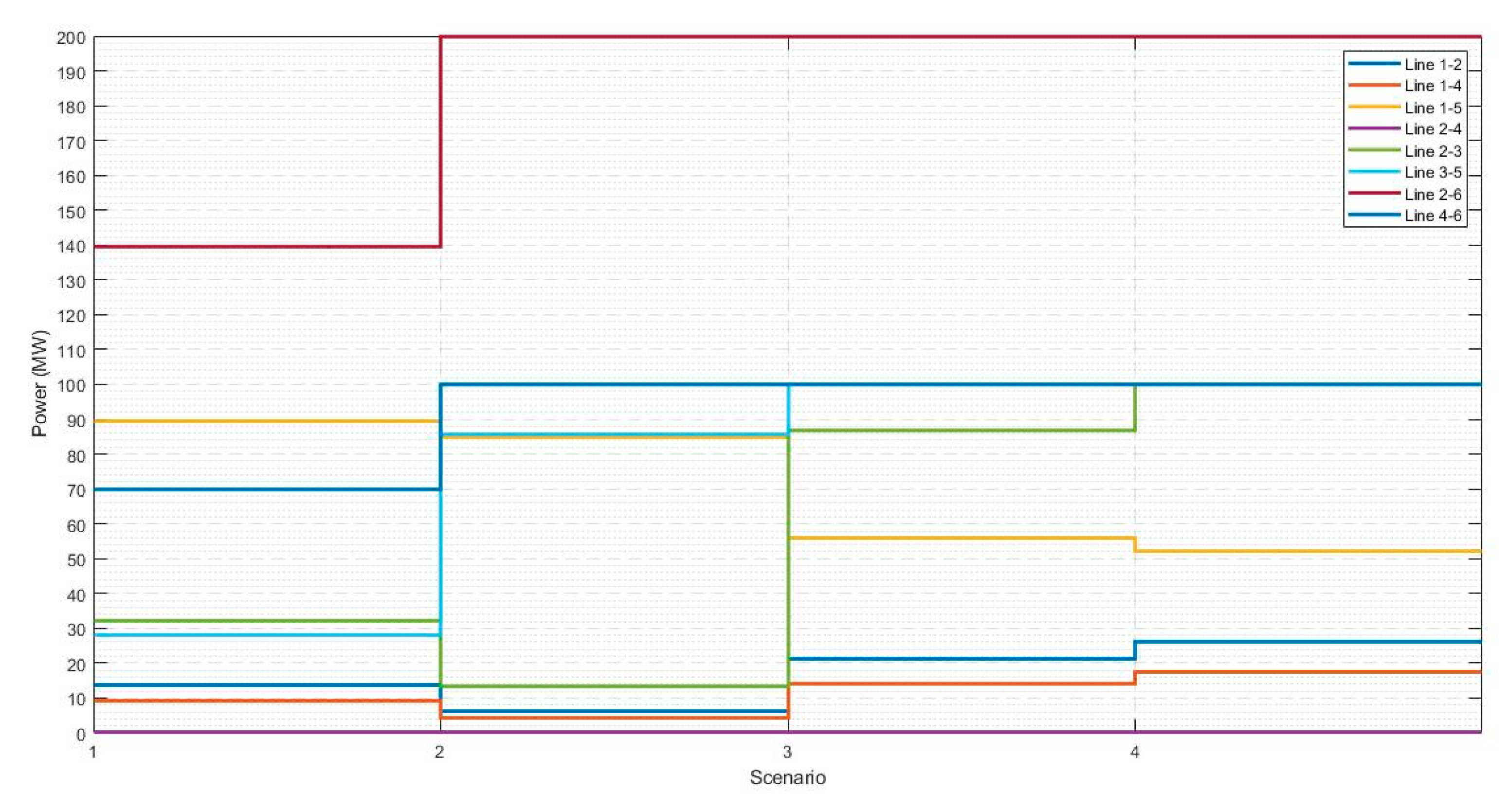
3.5.4. Case Study 3: Expansion with Multiple Planning Periods
4. Conclusions
Author Contributions
Funding
Conflicts of Interest
Notation
| Years | |
| Scenario e in year t | |
| Weight of scenario e in year t | |
| factor to make investment and operational costs comparable | |
| interest rate | |
| Demand block | |
| Generation block | |
| Battery | |
| Price bid of the i-th demand block in scenario c and year t | |
| Price offer of the i-th generation block in scenario c and year t | |
| Price offer of the i-th battery in node m for scenario c and year t | |
| Price bid of the i-th battery in node m for scenario c and year t | |
| Demand power by the i-th demand block in scenario c and year t | |
| Generated power by the i-th generation block in scenario c and year t | |
| Charge power battery n in node m for scenario c and year t | |
| Discharge power battery n in node m for scenario c and year t | |
| Annual amortization rate of the new lines | |
| Building cost of line k in corridor s-r | |
| Binary variable of line k in corridor s-r | |
| Factor accounting for the degradation of the battery | |
| Energy stored by the battery n in node m for scenario c and year t | |
| Price bid of the i-th demand block in scenario c. | |
| Binary variable that indicates if the battery is working in year t | |
| Cost per MWh in batteries | |
| Annual amortization rate of new batteries | |
| Set of years | |
| Set of scenarios | |
| Set of all charges | |
| Set of all generators | |
| Set of all batteries | |
| Set of new lines | |
| Set of new batteries | |
| Set of demand blocks connecting to node s | |
| Set of all generators at node s | |
| Set of all batteries at node s | |
| Set of all lines connecting to node s | |
| Power flow in line k of corridor s-r for scenario c and year t without considering losses | |
| Loss of power in line k of corridor s-r for scenario c and year t | |
| Power flow in line k of corridor s-r for scenario c and year t | |
| Voltage angle at node s | |
| Voltage angle at node r | |
| Independent variable assigned for the linearization of the losses | |
| Constant assigned to the slope of | |
| Number of linearization blocks (Number of partitions to approximate ) | |
| Binary variable equal to 1 when the battery is discharged | |
| Efficiency in battery discharge | |
| Efficiency in battery charging | |
| large positive constant | |
| Conductance between nodes s and r | |
| Suceptance between nodes s and r | |
| Voltage angle at node s | |
| Voltage angle at node r | |
| Losses of active power | |
| Lossless active power | |
| Voltage at node s | |
| Voltage at node r | |
| Complex power transmitted from node to node | |
| Active Power transmitted from node to node | |
| Reactive power transmitted from node to node | |
| Impedance between nodes and | |
| RL | Resistance of a transmission lines |
| XL | Inductive reactance of a transmission line |
References
- Gbadamosi, S.L.; Nwulu, N.I. A multi-period composite generation and transmission expansion planning model incorporating renewable energy sources and demand response. Sustain. Energy Technol. Assess. 2020, 39, 100726. [Google Scholar] [CrossRef]
- Maghouli, P.; Hosseini, S.H.; Buygi, M.O.; Shahidehpour, M. A multi-objective framework for transmission expansion planning in deregulated environments. IEEE Trans. Power Syst. 2009, 24, 1051–1061. [Google Scholar] [CrossRef]
- Rosellón, J. Different Approaches Towards Electricity Transmission Expansion. Rev. Netw. Econ. 2009, 2. [Google Scholar] [CrossRef]
- Lumbreras, S.; Ramos, A. The new challenges to transmission expansion planning. Survey of recent practice and literature review. Electr. Power Syst. Res. 2016, 134, 19–29. [Google Scholar] [CrossRef]
- Aguado, J.A.; de la Torre, S.; Triviño, A. Battery energy storage systems in transmission network expansion planning. Electr. Power Syst. Res. 2017, 145, 63–72. [Google Scholar] [CrossRef]
- Castro, T.E.G.; Jesus, L.L.M.; Trujillo, E.R. Literature review of BESS implementation in DER. Rev. Vínculos Cienc. Tecnol. Y Soc. 2019, 16, 321–326. [Google Scholar]
- Mazaheri, H.; Abbaspour, A.; Fotuhi-Firuzabad, M.; Farzin, H.; Moeini-Aghtaie, M. Investigating the impacts of energy storage systems on transmission expansion planning. In Proceedings of the 2017 25th Iranian Conference on Electrical Engineering, ICEE 2017, Tehran, Iran, 2–4 May 2017; pp. 1199–1203. [Google Scholar] [CrossRef]
- Denholm, P.; Sioshansi, R. The value of compressed air energy storage with wind in transmission-constrained electric power systems. Energy Policy 2009, 37, 3149–3158. [Google Scholar] [CrossRef]
- Wogrin, S.; Gayme, D.F. Optimizing Storage Siting, Sizing, and Technology Portfolios in Transmission-Constrained Networks. IEEE Trans. Power Syst. 2015, 30, 3304–3313. [Google Scholar] [CrossRef]
- Zhang, F.; Hu, Z.; Song, Y. Mixed-integer linear model for transmission expansion planning with line losses and energy storage systems. IET Gener. Transm. Distrib. 2013, 7, 919–928. [Google Scholar] [CrossRef]
- Worighi, I.; Maach, A.; Hafid, A.; Hegazy, O.; van Mierlo, J. Integrating renewable energy in smart grid system: Architecture, virtualization and analysis. Sustain. Energy Grids Netw. 2019, 18, 100226. [Google Scholar] [CrossRef]
- Nwulu, N.I.; Xia, X. Multi-objective dynamic economic emission dispatch of electric power generation integrated with game theory based demand response programs. Energy Convers. Manag. 2015, 89, 963–974. [Google Scholar] [CrossRef]
- Aguado, J.A.; de la Torre, S.; Contreras, J.; Conejo, A.J.; Martínez, A. Market-driven dynamic transmission expansion planning. Electr. Power Syst. Res. 2012, 82, 88–94. [Google Scholar] [CrossRef]
- de la Torre, S.; Conejo, A.J.; Contreras, J. Transmission expansion planning in electricity markets. IEEE Trans. Power Syst. 2008, 23, 238–248. [Google Scholar] [CrossRef]
- Latorre, G.; Cruz, R.D.; Areiza, J.M.; Villegas, A. Classification of publications and models on transmission expansion planning. IEEE Trans. Power Syst. 2003, 18, 938–946. [Google Scholar] [CrossRef]
- Garzillo, A.; Cazzol, M.V.; L’Abbate, A.; Migliavacca, G.; Mansoldox, A.; Riverax, A.; Nortonx, M. Offshore grids in Europe: The strategy of Ireland for 2020 and beyond. In Proceedings of the 9th IET International Conference on AC and DC Power Transmission (ACDC 2010), London, UK, 19–21 October 2010; Volume 2010, p. O64. [Google Scholar] [CrossRef]
- Alguacil, N.; Motto, A.L.; Conejo, A.J. Transmission expansion planning: A mixed-integer LP approach. IEEE Trans. Power Syst. 2003, 18, 1070–1077. [Google Scholar] [CrossRef]
- Zhang, H.; Heydt, G.T.; Vittal, V.; Quintero, J. An improved network model for transmission expansion planning considering reactive power and network losses. IEEE Trans. Power Syst. 2013, 28, 3471–3479. [Google Scholar] [CrossRef]
- Youssef, H.K.; Hackam, R. New transmission planning model. IEEE Trans. Power Syst. 1989, 4, 9–18. [Google Scholar] [CrossRef]
- Rahmani, M.; Rashidinejad, M.; Carreno, E.M.; Romero, R. Efficient method for AC transmission network expansion planning. Electr. Power Syst. Res. 2010, 80, 1056–1064. [Google Scholar] [CrossRef]
- Qiu, T.; Xu, B.; Wang, Y.; Dvorkin, Y.; Kirschen, D.S. Stochastic Multistage Coplanning of Transmission Expansion and Energy Storage. IEEE Trans. Power Syst. 2017, 32, 643–651. [Google Scholar] [CrossRef]
- Mexis, I.; Todeschini, G. Battery Energy Storage Systems in the United Kingdom: A Review of Current State-of-the-Art and Future Applications. Energies 2020, 13, 3616. [Google Scholar] [CrossRef]
- Tsianikas, S.; Zhou, J.; Iii, D.P.B.; Coit, D.W. Economic trends and comparisons for optimizing grid-outage resilient photovoltaic and battery systems. Appl. Energy 2019. [Google Scholar] [CrossRef]
- Marnell, K.; Obi, M.; Bass, R. Transmission-Scale Battery Energy Storage Systems: A Systematic Literature Review. Energies 2019, 12, 4603. [Google Scholar] [CrossRef]
- Villasana, R.; Salon, S.J.; Garver, L.L. Transmission network planning using linear programming. IEEE Trans. Power Appar. Syst. 1985, PAS-104, 349–356. [Google Scholar] [CrossRef]


| Node | Name | P (MW) | Offer Price | Name | P1 (MW) | P2 (MW) | Bid Price |
|---|---|---|---|---|---|---|---|
| 1 | G1 | 150 | 10 | D1 | 80 | 40 | 30, 28, 26, 24,20 |
| 2 | D2 | 240 | 120 | 34, 32, 30, 28, 25 | |||
| 3 | G2 | 120 | 20 | D3 | 40 | 20 | 20, 16, 14, 12, 10 |
| G3 | 120 | 22 | |||||
| G4 | 120 | 22 | |||||
| 4 | D4 | 160 | 80 | 30, 27, 24, 21, 17 | |||
| 5 | D5 | 240 | 120 | 34, 30, 26, 24, 18 | |||
| 6 | G5 | 100 | 8 | ||||
| G6 | 100 | 12 | |||||
| G7 | 100 | 15 | |||||
| G8 | 100 | 17 | |||||
| G9 | 100 | 19 | |||||
| G10 | 100 | 21 |
| Line | Cost (M$) | |||||
|---|---|---|---|---|---|---|
| 1–2 | 0.1 | 0.4 | −2.353 | 0.588 | 1 | 40 |
| 1–3 | 0.09 | 0.38 | −2.492 | 0.590 | 1 | 38 |
| 1–4 | 0.15 | 0.6 | −1.569 | 0.392 | 0.8 | 60 |
| 1–5 | 0.05 | 0.2 | −4.706 | 1.176 | 1 | 20 |
| 1–6 | 0.17 | 0.68 | −1.384 | 0.346 | 0.7 | 68 |
| 2–3 | 0.05 | 0.2 | −4.706 | 1.176 | 1 | 20 |
| 2–4 | 0.1 | 0.4 | −2.353 | 0.588 | 1 | 40 |
| 2–5 | 0.08 | 0.31 | −3.024 | 0.780 | 1 | 31 |
| 2–6 | 0.08 | 0.3 | −3.112 | 0.830 | 1 | 30 |
| 3–4 | 0.15 | 0.59 | −1.592 | 0.405 | 0.82 | 59 |
| 3–5 | 0.05 | 0.2 | −4.706 | 1.176 | 1 | 20 |
| 3–6 | 0.12 | 0.48 | −1.961 | 0.490 | 1 | 48 |
| 4–5 | 0.16 | 0.63 | −1.491 | 0.379 | 0.75 | 63 |
| 4–6 | 0.08 | 0.3 | −3.112 | 0.830 | 1 | 30 |
| 5–6 | 0.15 | 0.61 | −1.546 | 0.380 | 0.78 | 61 |
| Scenario | Demand Coefficient | Weight |
|---|---|---|
| 1 | 0.47 | 0.412 |
| 2 | 0.85 | 0.3297 |
| 3 | 1.2 | 0.1592 |
| 4 | 1.7 | 0.0991 |
| L | Number of Variables | Objective Function (M$) | Computing Time (s) | Energy Losses (%) |
|---|---|---|---|---|
| 1 | 1409 | 43.993 | 197.458 | 11.978 |
| 2 | 1553 | 51.337 | 114.513 | 7.246 |
| 4 | 1841 | 52.242 | 101.944 | 6.280 |
| 6 | 2129 | 52.503 | 107.414 | 5.968 |
| 8 | 2417 | 52.629 | 106.405 | 5.790 |
| 10 | 2705 | 52.631 | 136.018 | 5.708 |
| 20 | 4145 | 52.673 | 136.540 | 5.689 |
| 50 | 8465 | 52.687 | 265.359 | 5.691 |
| 100 | 15,665 | 52.688 | 237.754 | 5.716 |
| Scenario | Generated Energy (MWh) | Demanded Energy (MWh) | Energy Losses (MWh) | Energy Losses (%) | |
|---|---|---|---|---|---|
| Results Model | 1 | 355.300 | 338.500 | 16.8 | 4.728 |
| 2 | 551.100 | 517.000 | 34.100 | 6.188 | |
| 3 | 638.700 | 600.100 | 38.600 | 6.044 | |
| 4 | 650.000 | 610.100 | 39.900 | 6.138 | |
| Result Ref. [14] | 1 | 362.600 | 342.200 | 20.400 | 5.626 |
| 2 | 551.300 | 517.600 | 33.700 | 6.113 | |
| 3 | 637.600 | 600.100 | 37.500 | 5.881 | |
| 4 | 650.000 | 611.200 | 38.800 | 5.969 |
| Surplus Demand | Surplus Generators | Surplus Marketers | Investment Lines | Social Benefit Net | |
|---|---|---|---|---|---|
| Model results | 29.836 | 25.086 | 7.866 | 9.918 | 52.688 |
| Results Ref. [14] | 28 | 25.5 | 9.1 | 9.918 | 52.682 |
| Without Expansion | With Expansion | ||
|---|---|---|---|
| Number of new lines | - | 3 | |
| Net social welfare (M$) | 37.36 | 53.076 | |
| Total investment(M$) | - | 9.918 | |
| Metric | - | 2.586 | |
| - | 0.604 | ||
| - | 1.459 | ||
| - | 0.540 | ||
| Saturation index | 0.5393 | 0.47 | |
| Congestion index | 0.2048 | 0.092 |
| Scenario | Demand Coefficient | Weight |
|---|---|---|
| 1 | 1 | 1/6 |
| 2 | 1.67 | 1/6 |
| 3 | 3.33 | 1/6 |
| 4 | 2.33 | 1/6 |
| 5 | 2.67 | 1/6 |
| 6 | 2 | 1/6 |
| Cost ($/MWh) | Capacity (MWh) | Power (MW) | Offer Price ($/MWh) | Demand Price ($/MWh) | Capacity Degradation |
|---|---|---|---|---|---|
| 3000 | 40 | 10 | 27.5 | 22.5 | 1.1 |
| Line | Power Flow (MW) | |||||
|---|---|---|---|---|---|---|
| Scenario 1 | Scenario 2 | Scenario 3 | Scenario 4 | Scenario 5 | Scenario 6 | |
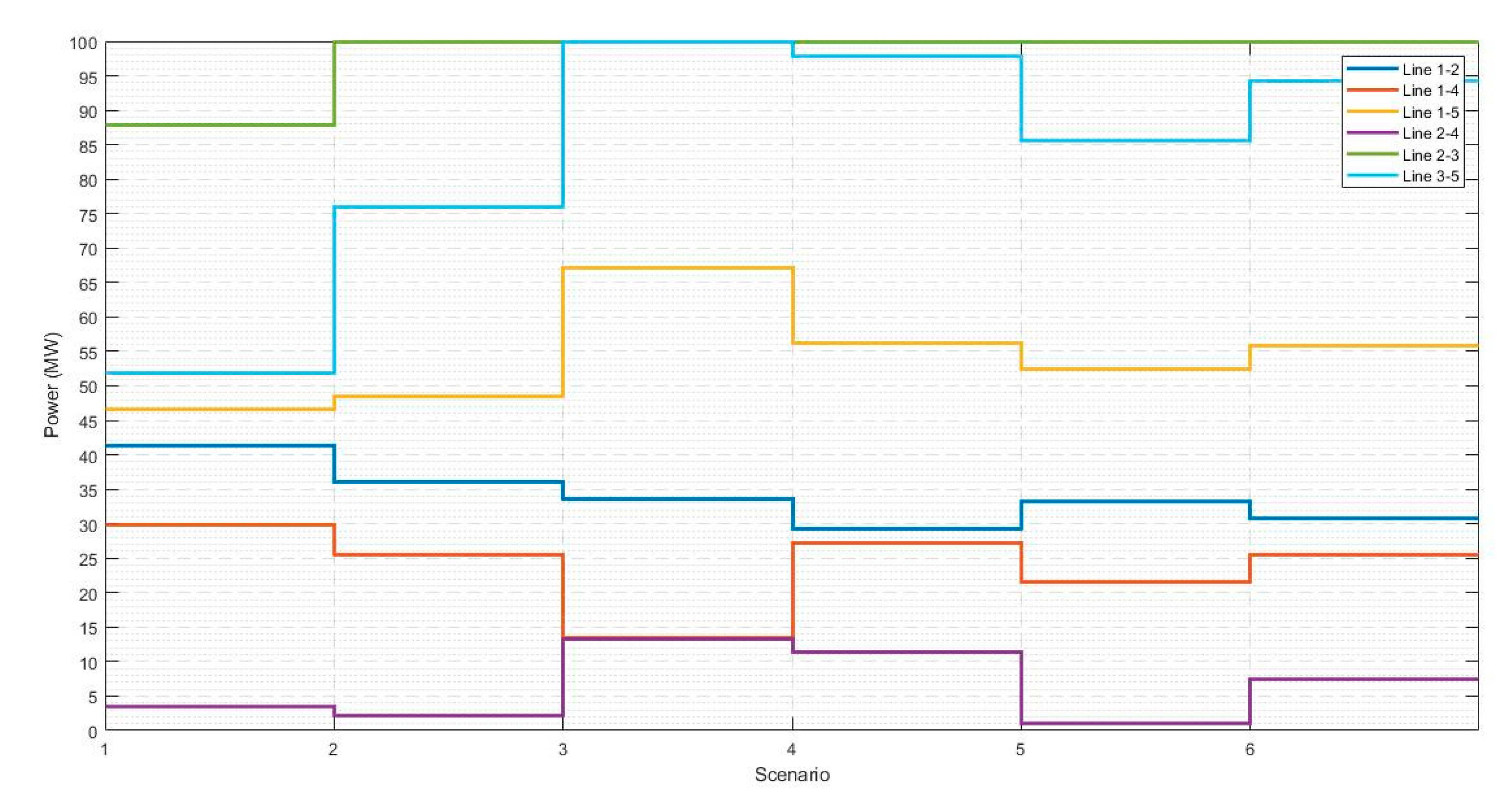
| 1–2 | 41.393 | 36.171 | 33.708 | 29.253 | 33.432 | 30.782 |
| 1–4 | 29.985 | 25.690 | 13.483 | 27.436 | 21.629 | 25.779 |
| 1–5 | 46.677 | 48.180 | 67.331 | 56.261 | 52.342 | 55.761 |
| 2–3 | 87.773 | 99.836 | 99.998 | 99.908 | 99.865 | 99.895 |
| 2–4 | 3.424 | 2.069 | 13.192 | 11.173 | 1.158 | 7.328 |
| 3–5 | 51.778 | 76.194 | 100.002 | 97.932 | 85.765 | 94.405 |
| Without Expansion | Expansion with Lines | Expansion with Lines and BESS | ||
|---|---|---|---|---|
| Number of new lines | - | 3 | 3 | |
| Number of new batteries | - | - | 4 | |
| Net social welfare (M$) | 40.48 | 61.916 | 62.122 | |
| Investment in lines (M$) | - | 9.918 | 9.918 | |
| Investment in battery (M$) | - | 0.085905 | ||
| Total investment (M$) | 9.918 | 10.00391 | ||
| Metrics | - | 3.1613 | 3.1633 | |
| - | 0.7725 | 0.4977 | ||
| 0.4977 | ||||
| - | 1.3072 | 1.4936 | ||
| - | 1.0808 | 1.3925 | ||
| Saturation index | 0.5644 | 0.6781 | 0.686 | |
| Congestion index | 0.2055 | 0.07598 | 0.098 |
| Without Expansion | Expansion with Lines | Expansion with Lines and BESS | ||
|---|---|---|---|---|
| Number of new lines | - | 5 | 5 | |
| Number of new batteries | - | - | 4 | |
| Investment in lines (M$) | - | 76.164 | 76.164 | |
| Investment in batteries (M$) | - | - | 0.085905 | |
| Net social welfare (M$) | 300.037 | 478.624 | 479.726 | |
| Surplus generator (M$) | 140.244 | 205.849 | 202.713 | |
| Surplus demands (M$) | 141.132 | 278.606 | 202.713 | |
| Surplus batteries (M$) | - | - | 1.152 | |
| Surplus marketer (M$) | 18.660 | 70.333 | 73.332 | |
| Total investment (M$) | - | 76.164 | 76.668 | |
| Metrics | 3.344 | 3.344 | ||
| - | 0.861 | 0.814 | ||
| - | - | 0.829 | ||
| - | 1.804 | 1.800 | ||
| - | 0.678 | 0.713 |
| Scenario 1 | 150 | 150.56 | 0.56 |
| Scenario 2 | 150 | 152.011 | 2.011 |
| Scenario 3 | 150 | 152.33 | 2.033 |
| Scenario 4 | 150 | 151.971 | 1.971 |
| Scenario 5 | 150 | 152.6 | 2.6 |
| Scenario 6 | 150 | 151.81 | 1.81 |
© 2020 by the authors. Licensee MDPI, Basel, Switzerland. This article is an open access article distributed under the terms and conditions of the Creative Commons Attribution (CC BY) license (http://creativecommons.org/licenses/by/4.0/).
Share and Cite
Mora, C.A.; Montoya, O.D.; Trujillo, E.R. Mixed-Integer Programming Model for Transmission Network Expansion Planning with Battery Energy Storage Systems (BESS). Energies 2020, 13, 4386. https://doi.org/10.3390/en13174386
Mora CA, Montoya OD, Trujillo ER. Mixed-Integer Programming Model for Transmission Network Expansion Planning with Battery Energy Storage Systems (BESS). Energies. 2020; 13(17):4386. https://doi.org/10.3390/en13174386
Chicago/Turabian StyleMora, Camilo Andres, Oscar Danilo Montoya, and Edwin Rivas Trujillo. 2020. "Mixed-Integer Programming Model for Transmission Network Expansion Planning with Battery Energy Storage Systems (BESS)" Energies 13, no. 17: 4386. https://doi.org/10.3390/en13174386
APA StyleMora, C. A., Montoya, O. D., & Trujillo, E. R. (2020). Mixed-Integer Programming Model for Transmission Network Expansion Planning with Battery Energy Storage Systems (BESS). Energies, 13(17), 4386. https://doi.org/10.3390/en13174386