Mapping and Spatial Analysis of Electricity Load Shedding Experiences: A Case Study of Communities in Accra, Ghana


Abstract
:1. Introduction
Spatial Approaches in Energy Studies
2. Study Area and Data
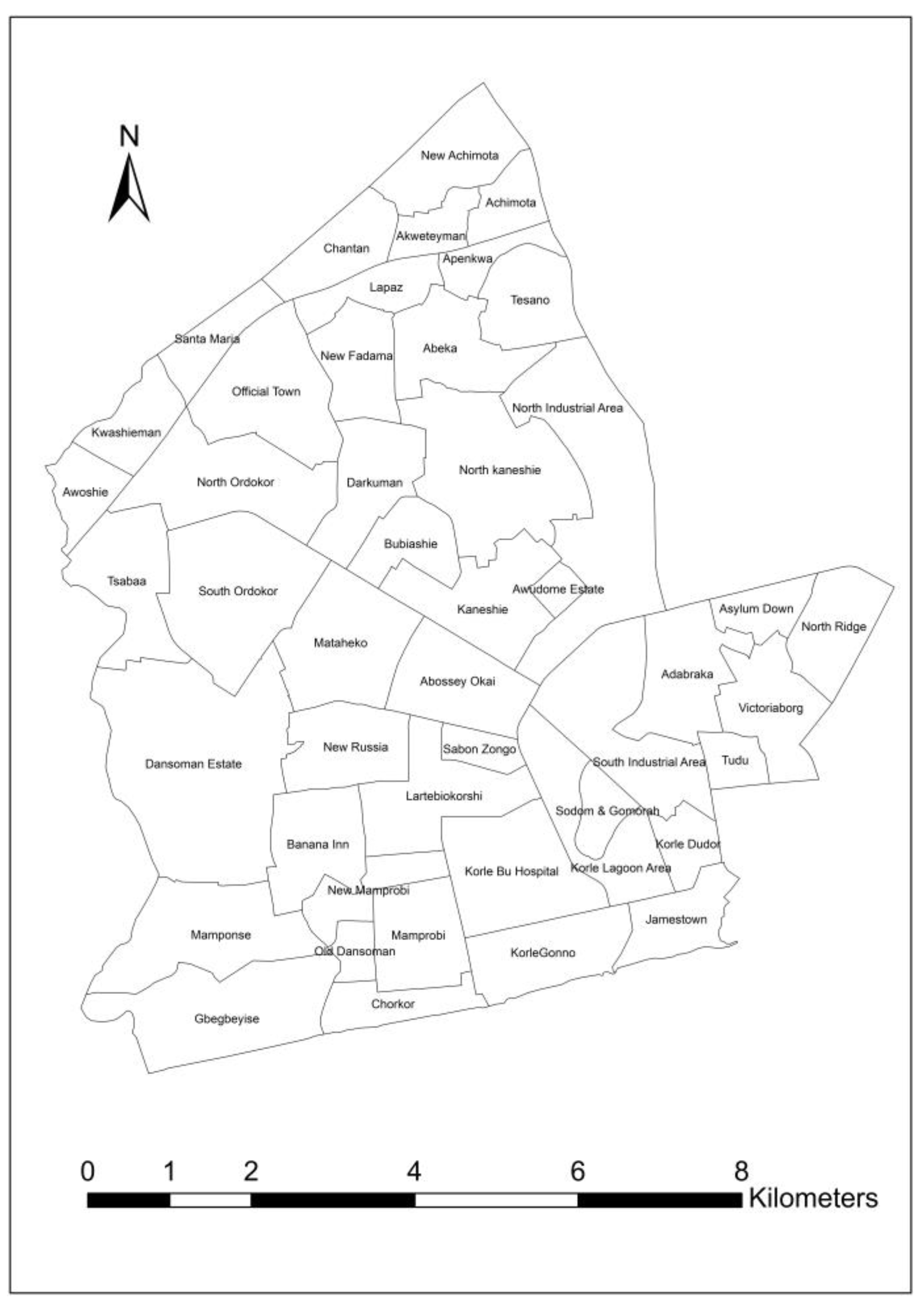
2.1. Study Area
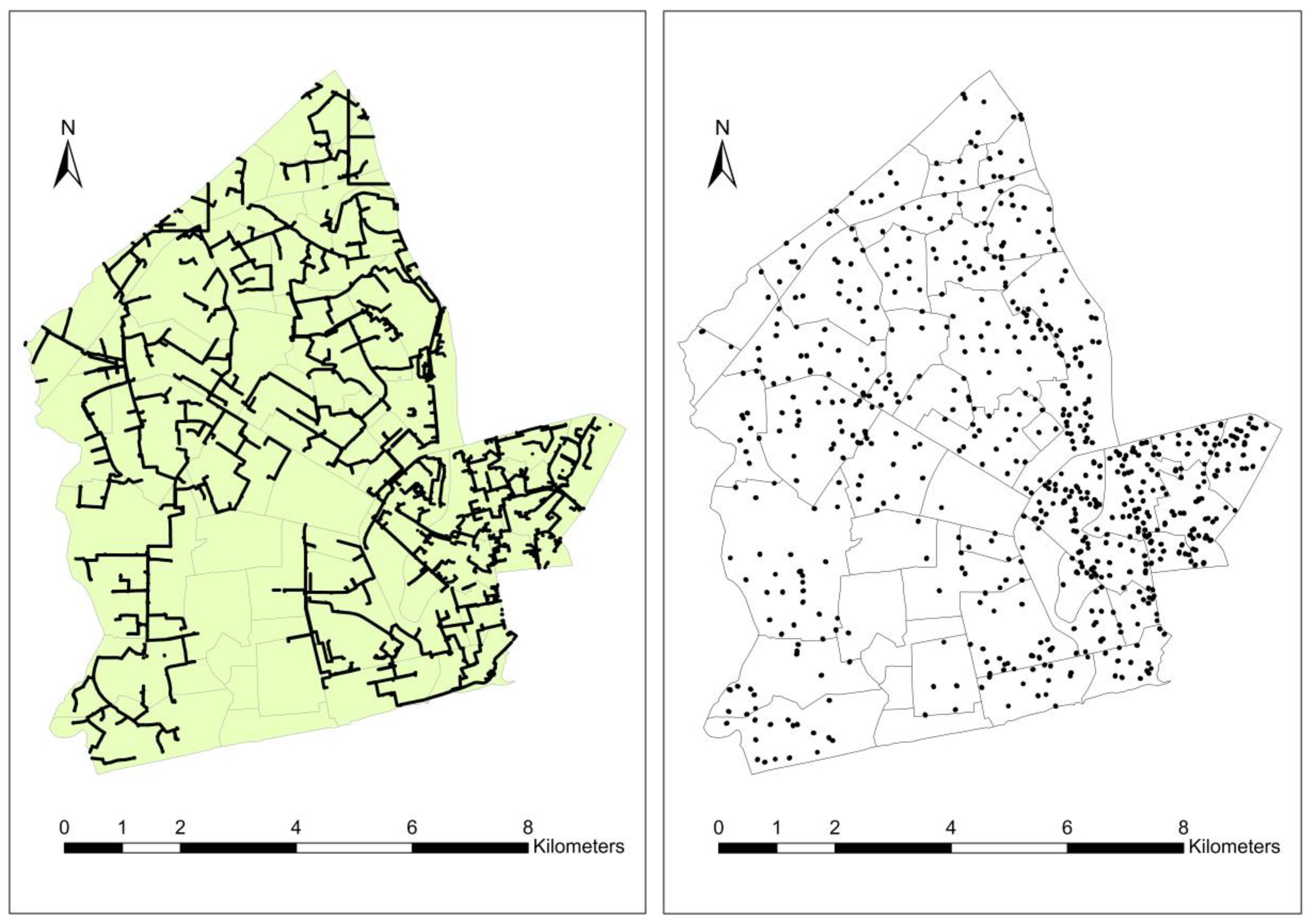
2.2. Data and Data Sources
2.3. Mapping Neighborhood Load Shedding Outage Experiences
3. Methods
3.1. Calculating Neighbourhood Load Shedding Exposure and Normalization
3.2. Spatial Analysis
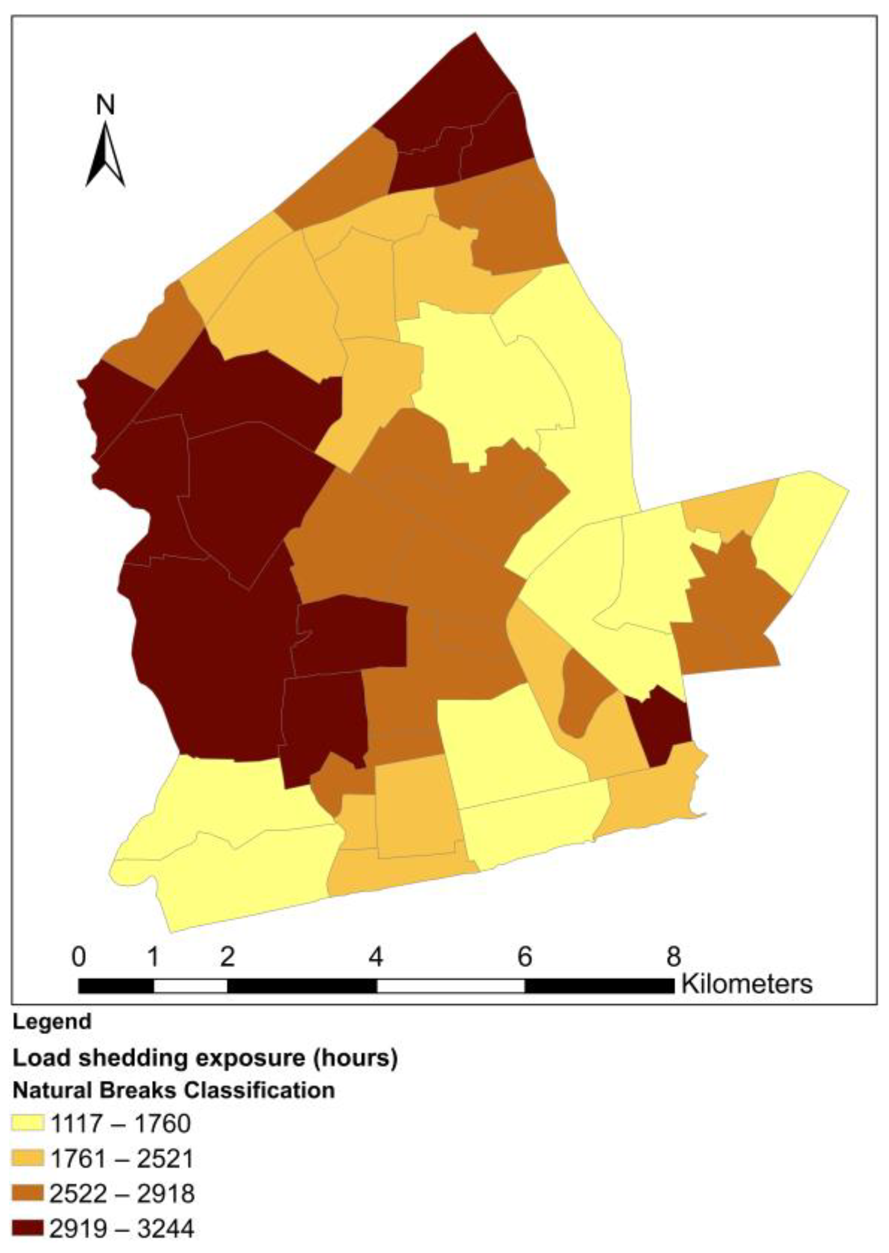
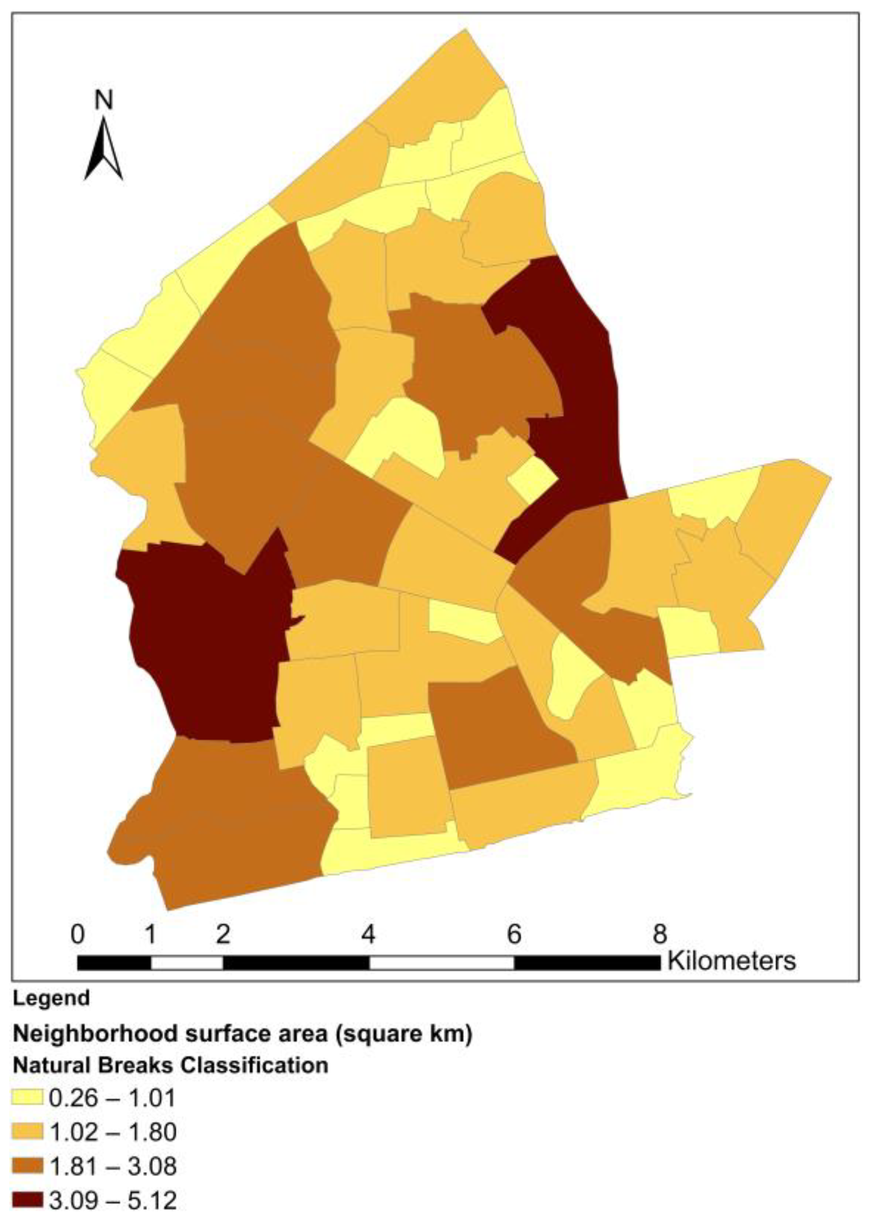
3.2.1. Visualization
3.2.2. Global index of Spatial Autocorrelation
3.2.3. Local Indicators of Spatial Autocorrelation
3.2.4. Conceptualization of Spatial Relationships
4. Results and Discussion
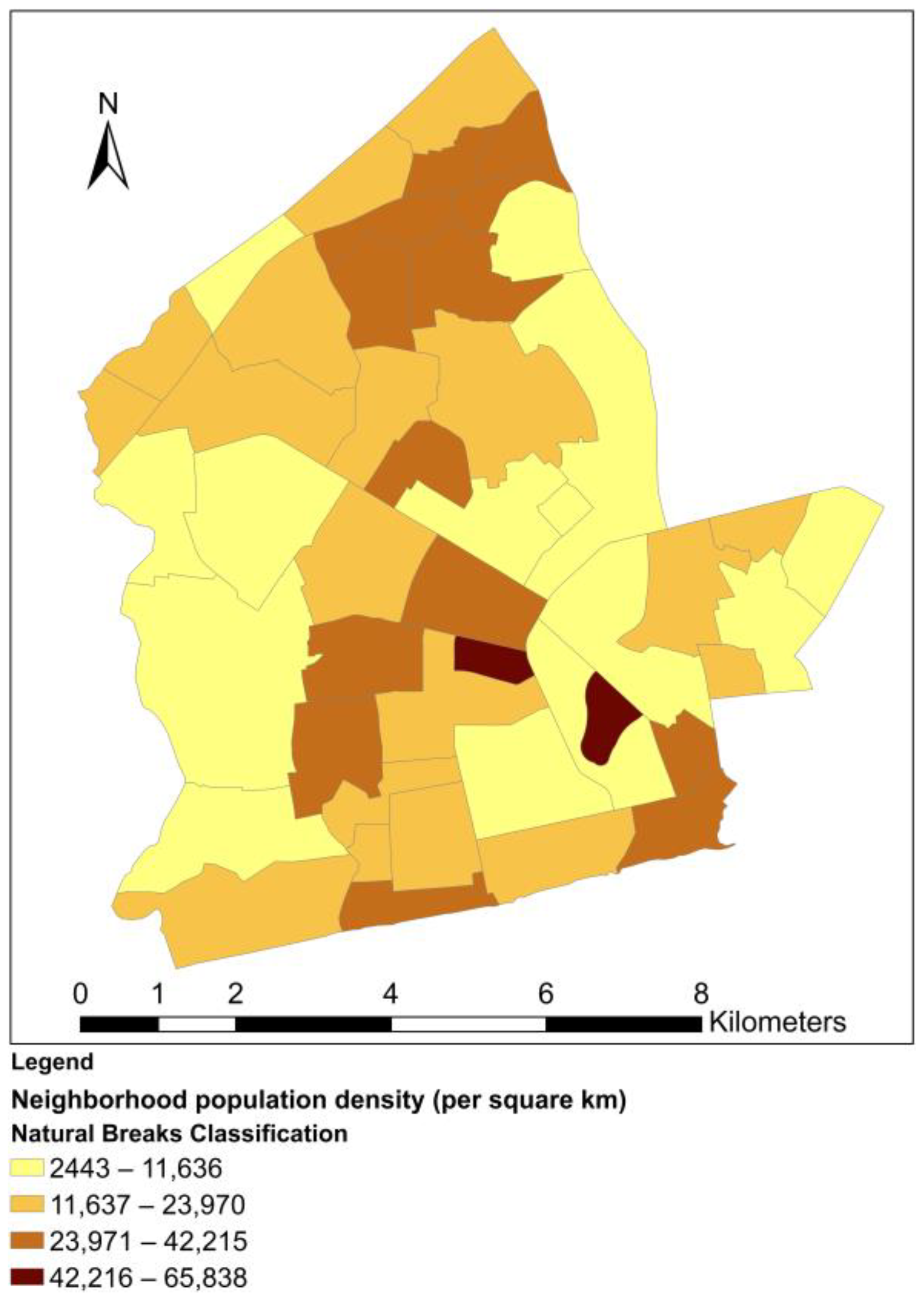
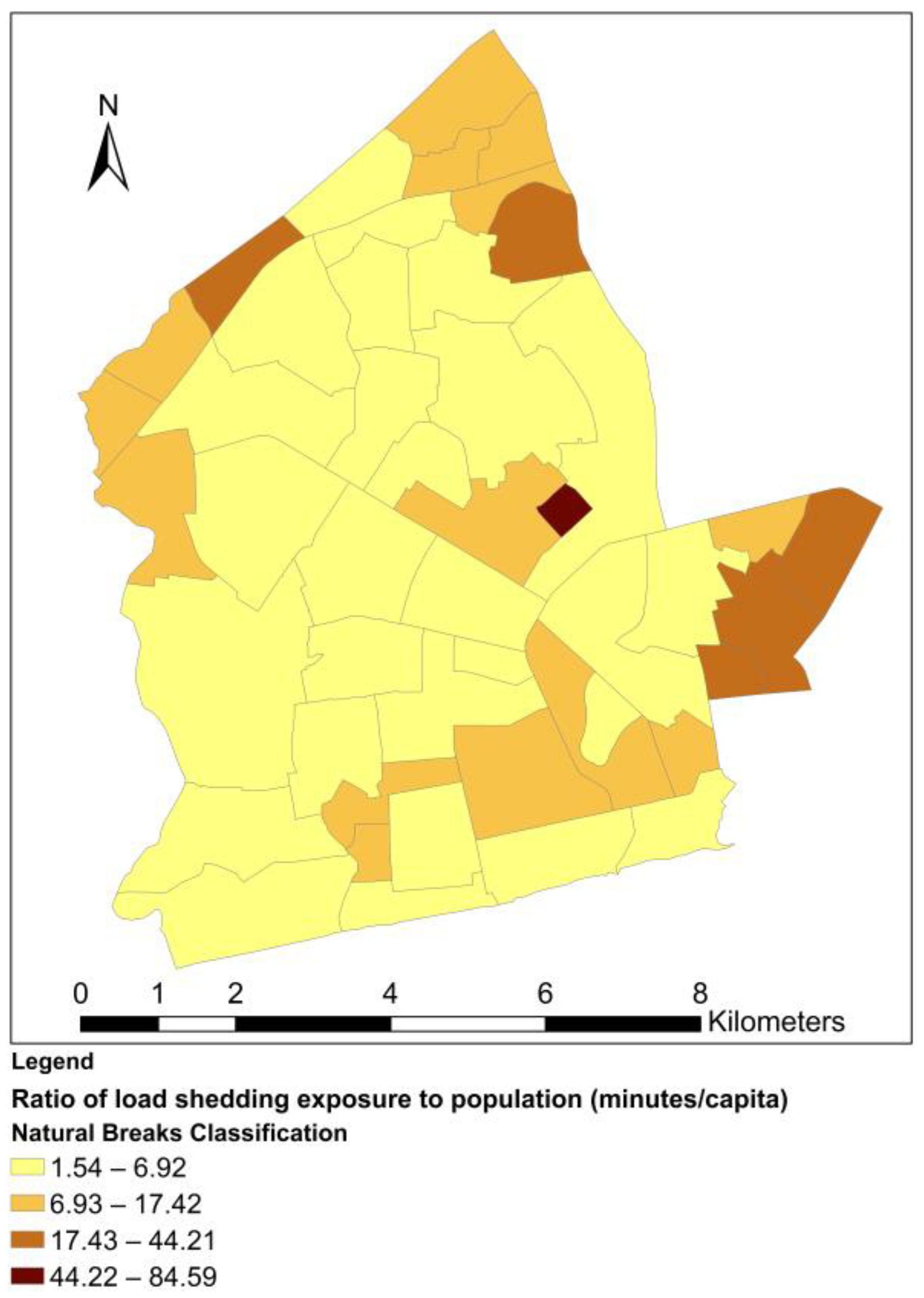
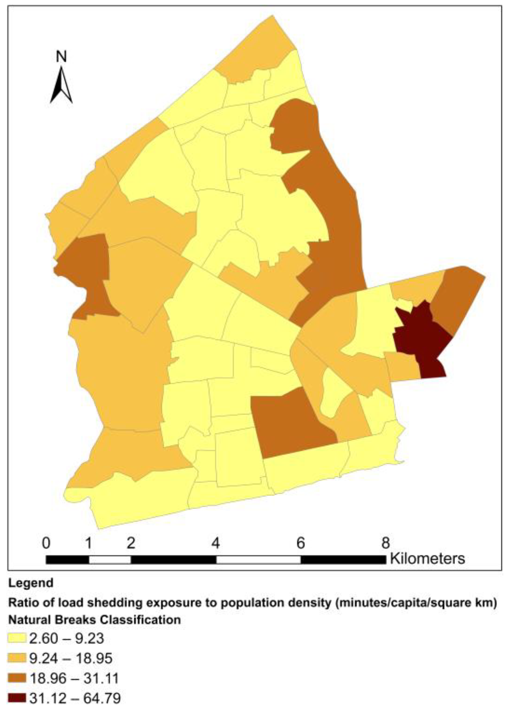
4.1. Calculating, Normalizing and Visualizing Load Shedding Exposure
4.2. Global Spatial Autocorrelation of Load Shedding Exposure
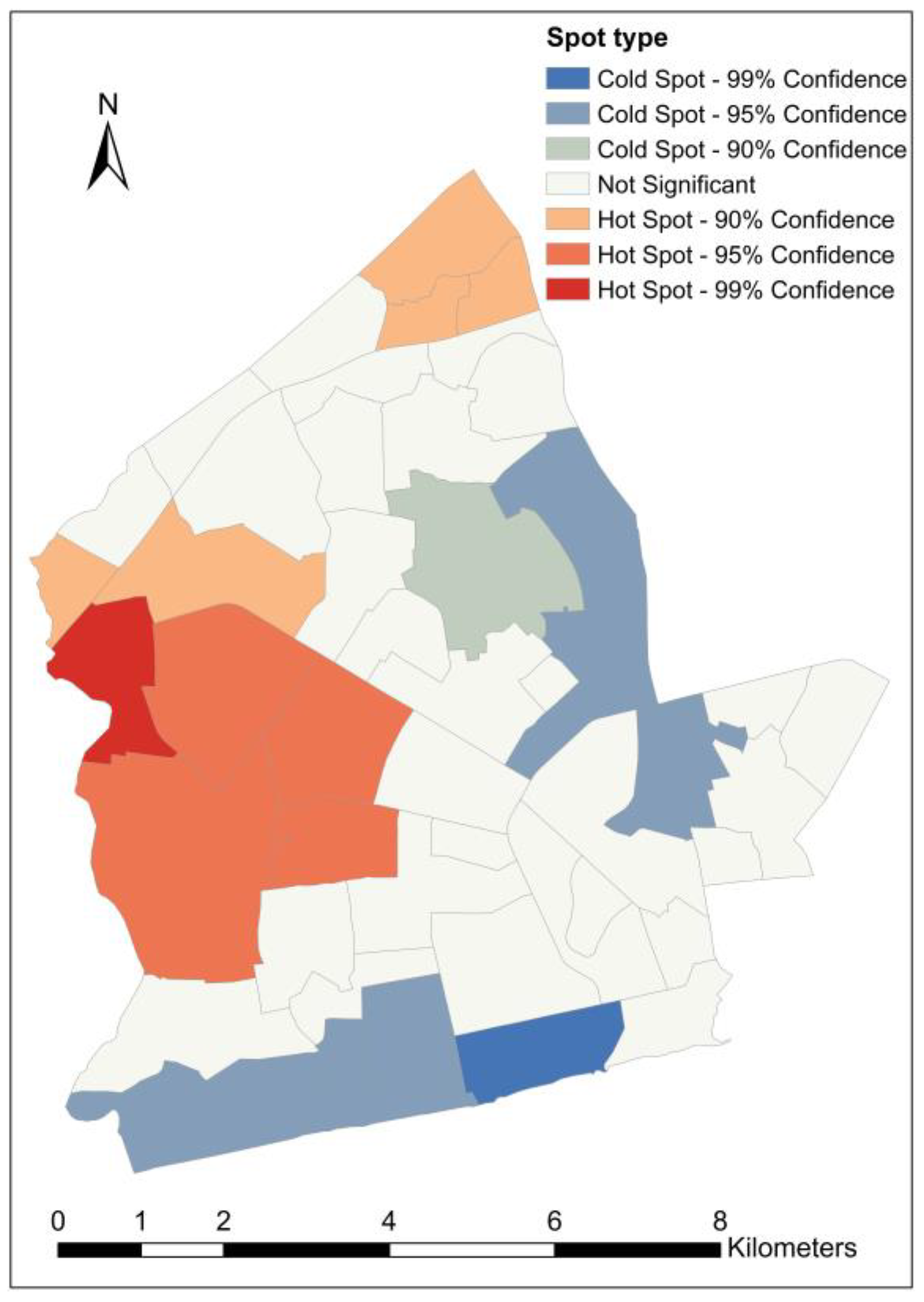
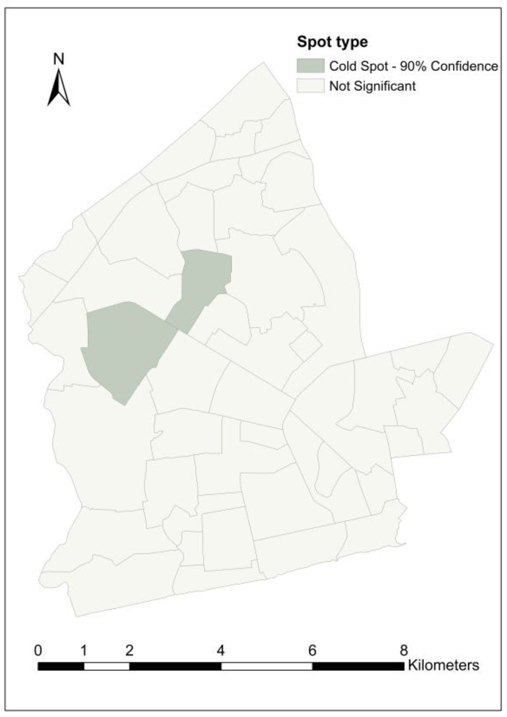
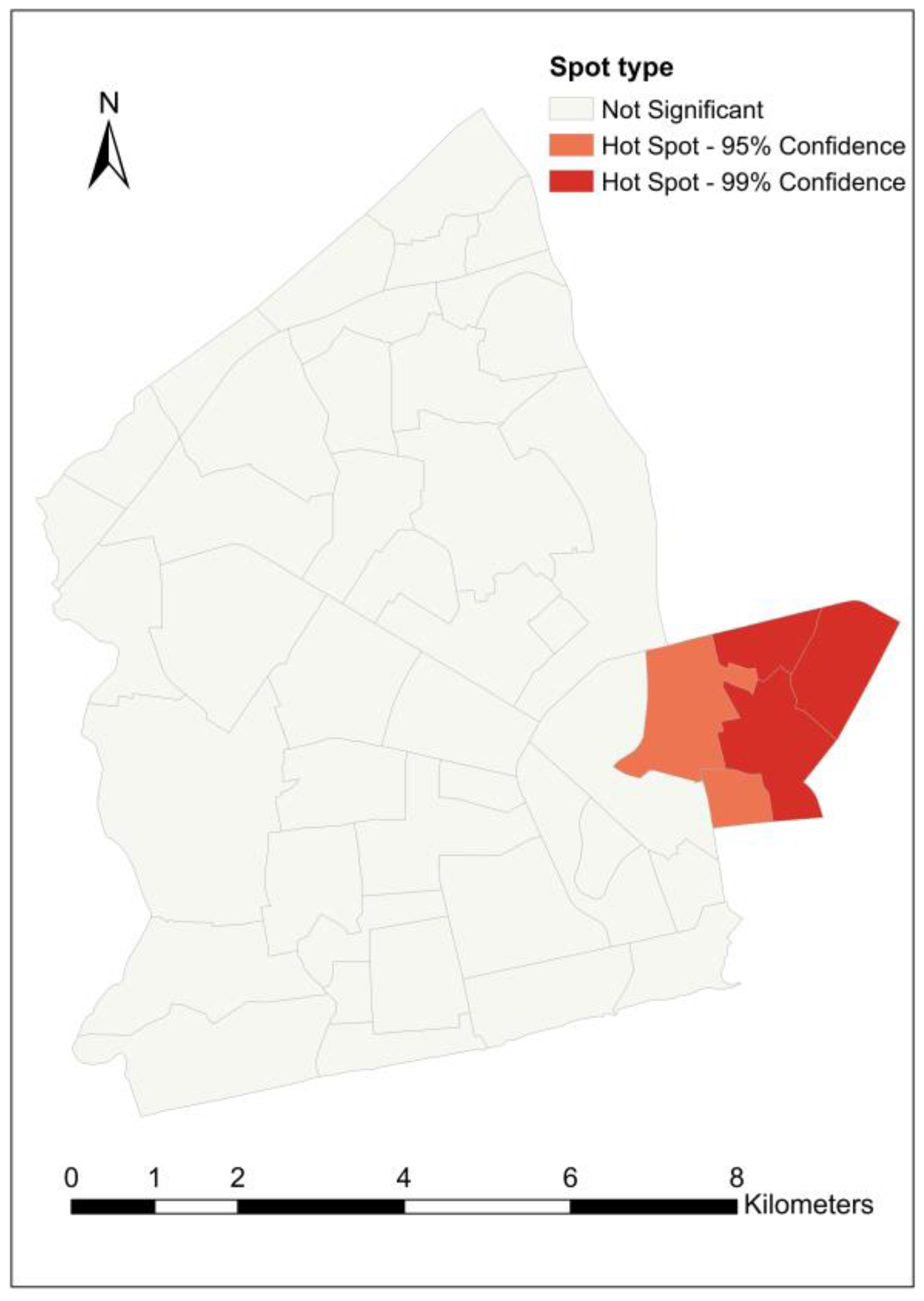
4.3. Hot Spot Analysis
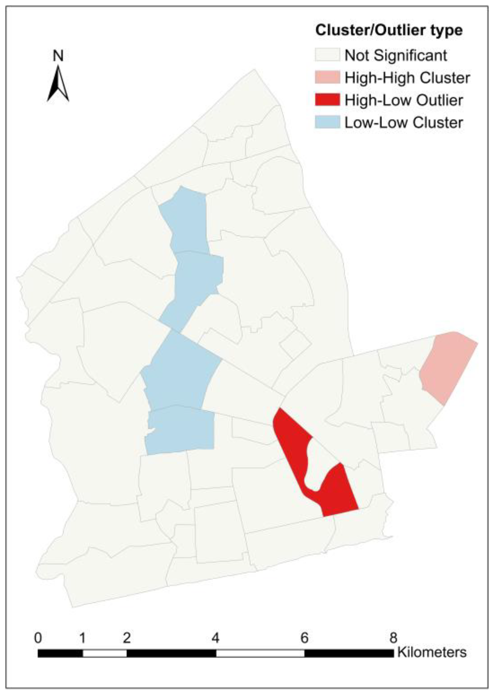
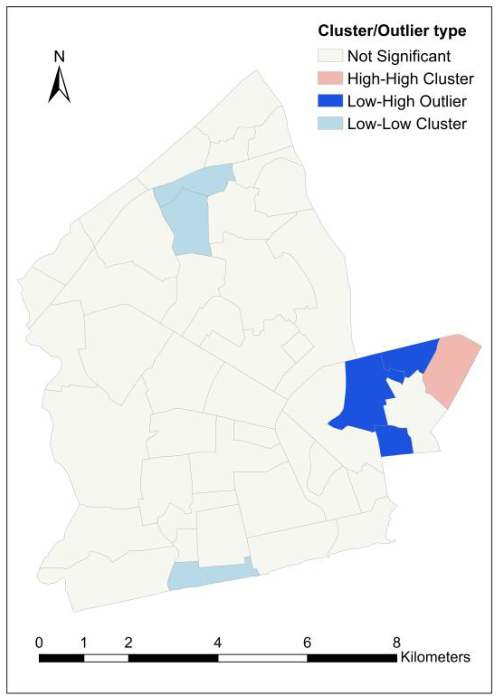
4.4. Cluster and Outlier Analysis
4.5. Comparing Results from Local Indicators of Spatial Association (LISA) Analyses
4.6. Comparing Visualization and Spatial Statistical Analysis Results
5. Conclusions, Limitations and Future Research
Author Contributions
Funding
Acknowledgments
Conflicts of Interest
References
- Ghanem, D.A.; Mander, S.; Gough, C. “I think we need to get a better generator”: Household resilience to disruption to power supply during storm events. Energy Policy 2016, 92, 171–180. [Google Scholar] [CrossRef]
- Mitsova, D.; Esnard, A.-M.; Sapat, A.; Lai, B.S. Socioeconomic vulnerability and electric power restoration timelines in Florida: The case of Hurricane Irma. Nat. Hazards 2018, 94, 689–709. [Google Scholar] [CrossRef]
- Hines, P.; Apt, J.; Talukdar, S. Large blackouts in North America: Historical trends and policy implications. Energy Policy 2009, 37, 5249–5259. [Google Scholar] [CrossRef]
- Panteli, M.; Mancarella, P. Influence of extreme weather and climate change on the resilience of power systems: Impacts and possible mitigation strategies. Electr. Power Syst. Res. 2015, 127, 259–270. [Google Scholar] [CrossRef]
- Hiete, M.; Merz, M.; Schultmann, F. Scenario-based impact analysis of a power outage on healthcare facilities in Germany. Int. J. Disaster Resil. Built Environ. 2011, 2, 222–244. [Google Scholar] [CrossRef]
- Aidoo, K.; Briggs, R.C. Underpowered: Rolling blackouts in Africa disproportionately hurt the poor. Afr. Stud. Rev. 2019, 62, 112–131. [Google Scholar] [CrossRef]
- Paradi-Guilford, C. How Ghana Is Tackling Energy Shortages. Available online: https://www.weforum.org/agenda/2015/03/how-ghana-is-tackling-energy-shortages/ (accessed on 25 March 2015).
- Andersen, T.B.; Dalgaard, C.-J. Power outages and economic growth in Africa. Energy Econ. 2013, 38, 19–23. [Google Scholar] [CrossRef] [Green Version]
- Cole, M.A.; Elliott, R.J.; Occhiali, G.; Strobl, E. Power outages and firm performance in Sub-Saharan Africa. J. Dev. Econ. 2018, 134, 150–159. [Google Scholar] [CrossRef]
- Moyo, B. Power infrastructure quality and manufacturing productivity in Africa: A firm level analysis. Energy Policy 2013, 61, 1063–1070. [Google Scholar] [CrossRef]
- Diboma, B.; Tatietse, T.T. Power interruption costs to industries in Cameroon. Energy Policy 2013, 62, 582–592. [Google Scholar] [CrossRef]
- Farquharson, D.; Jaramillo, P.; Samaras, C. Sustainability implications of electricity outages in sub-Saharan Africa. Nat. Sustain. 2018, 1, 589–597. [Google Scholar] [CrossRef]
- Mensah, J.T. Jobs! Electricity Shortages and Unemployment in Africa; World Bank Group: Washington, DC, USA, 2018. [Google Scholar]
- PULSE. Dumsor Cost Us $3Billion—Nana Addo. Available online: https://www.pulse.com.gh/news/business/power-crisis-dumsor-cost-us-dollar3billion-nana-addo/m0ye2mc (accessed on 17 August 2017).
- Kamasa, K.; Adu, G.; Oteng-Abayie, E. Business environment and firms’ decisions to evade taxes: Evidence from Ghana. Afr. J. Bus. Econ. Res. 2019, 14, 135–155. [Google Scholar] [CrossRef]
- Dzansi, J.; Puller, S.L.; Street, B.; Yebuah-Dwamena, B. The Vicious Circle of Blackouts and Revenue Collection in Developing Economies: Evidence from Ghana (E-89457-GHA-1); International Growth Centre: London, UK, 2018. [Google Scholar]
- Apenteng, B.A.; Opoku, S.T.; Ansong, D.; Akowuah, E.A.; Afriyie-Gyawu, E. The effect of power outages on in-facility mortality in healthcare facilities: Evidence from Ghana. Glob. Public Health 2018, 13, 545–555. [Google Scholar] [CrossRef] [PubMed]
- Bayor, I.; Yelyang, A. The Ghana “Dumsor” Energy Setbacks and Sensitivities: From Confrontation to Collaboration; West Africa Network for Peacebuilding (WANEP): Accra, Ghana, 2015. [Google Scholar]
- Liévanos, R.S.; Horne, C. Unequal resilience: The duration of electricity outages. Energy Policy 2017, 108, 201–211. [Google Scholar] [CrossRef]
- Maliszewski, P.J.; Perrings, C. Factors in the resilience of electrical power distribution infrastructures. Appl. Geogr. 2012, 32, 668–679. [Google Scholar] [CrossRef]
- Kesselring, R. The electricity crisis in Zambia: Blackouts and social stratification in new mining towns. Energy Res. Soc. Sci. 2017, 30, 94–102. [Google Scholar] [CrossRef] [Green Version]
- Min, B. Political Favoritism and the Targeting of Power Outages; International Growth Centre: London, UK, 2019. [Google Scholar]
- De Oliveira, V.H.; de Medeiros, C.N.; Carvalho, J.R. Violence and local development in Fortaleza, Brazil: A spatial regression analysis. Appl. Spat. Anal. 2019, 12, 147–166. [Google Scholar] [CrossRef]
- Tu, W.; Tedders, S.; Tian, J. An exploratory spatial data analysis of low birth weight prevalence in Georgia. Appl. Geogr. 2012, 32, 195–207. [Google Scholar] [CrossRef]
- Rodríguez-Pose, A.; Tselios, V. Mapping the European regional educational distribution. Eur. Urban Reg. Stud. 2011, 18, 358–374. [Google Scholar] [CrossRef]
- Sharma, A. Exploratory spatial data analysis of older adult migration: A case study of North Carolina. Appl. Geogr. 2012, 35, 327–333. [Google Scholar] [CrossRef]
- Vidyattama, Y.; Li, J.; Miranti, R. Measuring spatial distributions of secondary education achievement in Australia. Appl. Spat. Anal. 2019, 12, 493–514. [Google Scholar] [CrossRef]
- Nunes, L.; Lourenço, L.; Meira, A.C. Exploring spatial patterns and drivers of forest fires in Portugal (1980–2014). Sci. Total Environ. 2016, 573, 1190–1202. [Google Scholar] [CrossRef] [PubMed]
- Tsai, P.-J.; Lin, M.-L.; Chu, C.-M.; Perng, C.-H. Spatial autocorrelation analysis of health care hotspots in Taiwan in 2006. BMC Public Health 2009, 9, 464. [Google Scholar] [CrossRef] [PubMed] [Green Version]
- López-Carr, D.; Pricope, N.G.; Aukema, J.E.; Jankowska, M.M.; Funk, C.; Husak, G.; Michaelsen, J. Spatial analysis of population dynamics and climate change in Africa: Potential vulnerability hot spots emerge where precipitation declines and demographic pressures coincide. Popul. Environ. 2014, 35, 323–339. [Google Scholar] [CrossRef]
- Hession, S.L.; Moore, N. A spatial regression analysis of the influence of topographyon monthly rainfall in East Africa. Int. J. Climatol. 2011, 31, 1440–1456. [Google Scholar] [CrossRef]
- Ansong, D.; Ansong, E.K.; Ampomah, A.O.; Afranie, S. A spatio-temporal analysis of academic performance at the Basic Education Certificate Examination in Ghana. Appl. Geogr. 2015, 65, 1–12. [Google Scholar] [CrossRef]
- Boyda, D.C.; Holzman, S.B.; Berman, A.; Grabowski, M.K.; Chang, L.W. Geographic information systems, spatial analysis, and HIV in Africa: A scoping review. PLoS ONE 2019, 14, e0216388. [Google Scholar] [CrossRef]
- Ramachandra, T.; Shruthi, B. Spatial mapping of renewable energy potential. Renew. Sustain. Energy Rev. 2007, 11, 1460–1480. [Google Scholar] [CrossRef]
- Güngör-Demirci, G. Spatial analysis of renewable energy potential and use in Turkey. J. Renew. Sustain. Energy 2015, 7, 013126(1)–013126(17). [Google Scholar]
- Arnette, N.; Zobel, C.W. Spatial analysis of renewable energy potential in the greater southern Appalachian mountains. Renew. Energy 2011, 36, 2785–2798. [Google Scholar] [CrossRef]
- Wang, Q.; Kwan, M.-P.; Fan, J.; Zhou, K.; Wang, Y.-F. A study on the spatial distribution of the renewable energy industries in China and their driving factors. Renew. Energy 2019, 139, 161–175. [Google Scholar] [CrossRef]
- Xie, H.; Liu, G.; Liu, Q.; Wang, P. Analysis of spatial disparities and driving factors of energy consumption change in China based on spatial statistics. Sustainability 2014, 6, 2264–2280. [Google Scholar] [CrossRef] [Green Version]
- Walker, R.; McKenzie, P.; Liddell, C.; Morris, C. Spatial analysis of residential fuel prices: Local variations in the price of heating oil in Northern Ireland. Appl. Geogr. 2015, 63, 369–379. [Google Scholar] [CrossRef]
- Dar-Mousa, R.N.; Makhamreh, Z. Analysis of the pattern of energy consumptions and its impact on urban environmental sustainability in Jordan: Amman City as a case study. Energy Sustain. Soc. 2019, 9, 15. [Google Scholar] [CrossRef] [Green Version]
- Tyralis, H.; Mamassis, N.; Photis, Y.N. Spatial analysis of the electrical energy demand in Greece. Energy Policy 2017, 102, 340–352. [Google Scholar] [CrossRef]
- Parry, D.; Cowley, C. Maps as a technique for visualizing load-shedding schedules. In Proceedings of the 2015 Annual Conference of the South African Institute of Computer Scientists and Information Technologists: Knowledge through Technology (SAICSIT 2015), Stellenbosch, South Africa, 28–30 September 2015. [Google Scholar]
- GSS. Demography: Population Projection. Available online: http://www.statsghana.gov.gh/nationalaccount_macros.php?Stats=MTA1NTY1NjgxLjUwNg==/webstats/s679n2sn87 (accessed on 14 August 2019).
- Engstrom, R.; Ofiesh, C.; Rain, D.; Jewell, H.; Weeks, J. Defining neighborhood boundaries for urban health research in developing countries: A case study of Accra, Ghana. J. Maps 2013, 9, 36–42. [Google Scholar] [CrossRef] [Green Version]
- Waller, L.A.; Gotway, C.A. Applied Spatial Statistics for Public Health Data; John Wiley and Sons: New York, NY, USA, 2004. [Google Scholar]
- ESRI. How Spatial Autocorrelation (Global Moran’s I) Works: ArcMap. Available online: https://desktop.arcgis.com/en/arcmap/10.5/tools/spatial-statistics-toolbox/h-how-spatial-autocorrelation-moran-s-i-spatial-st.htm (accessed on 10 May 2018).
- Getis, A.; Ord, J.K. The analysis of spatial association by use of distance statistics. Geogr. Anal. 1992, 24, 189–206. [Google Scholar] [CrossRef]
- Anselin, L. Local Indicators of Spatial Association—LISA. Geogr. Anal. 1995, 27, 93–115. [Google Scholar] [CrossRef]


| Variable | Unit of Measurement |
|---|---|
| Neighborhood surface area | km2 |
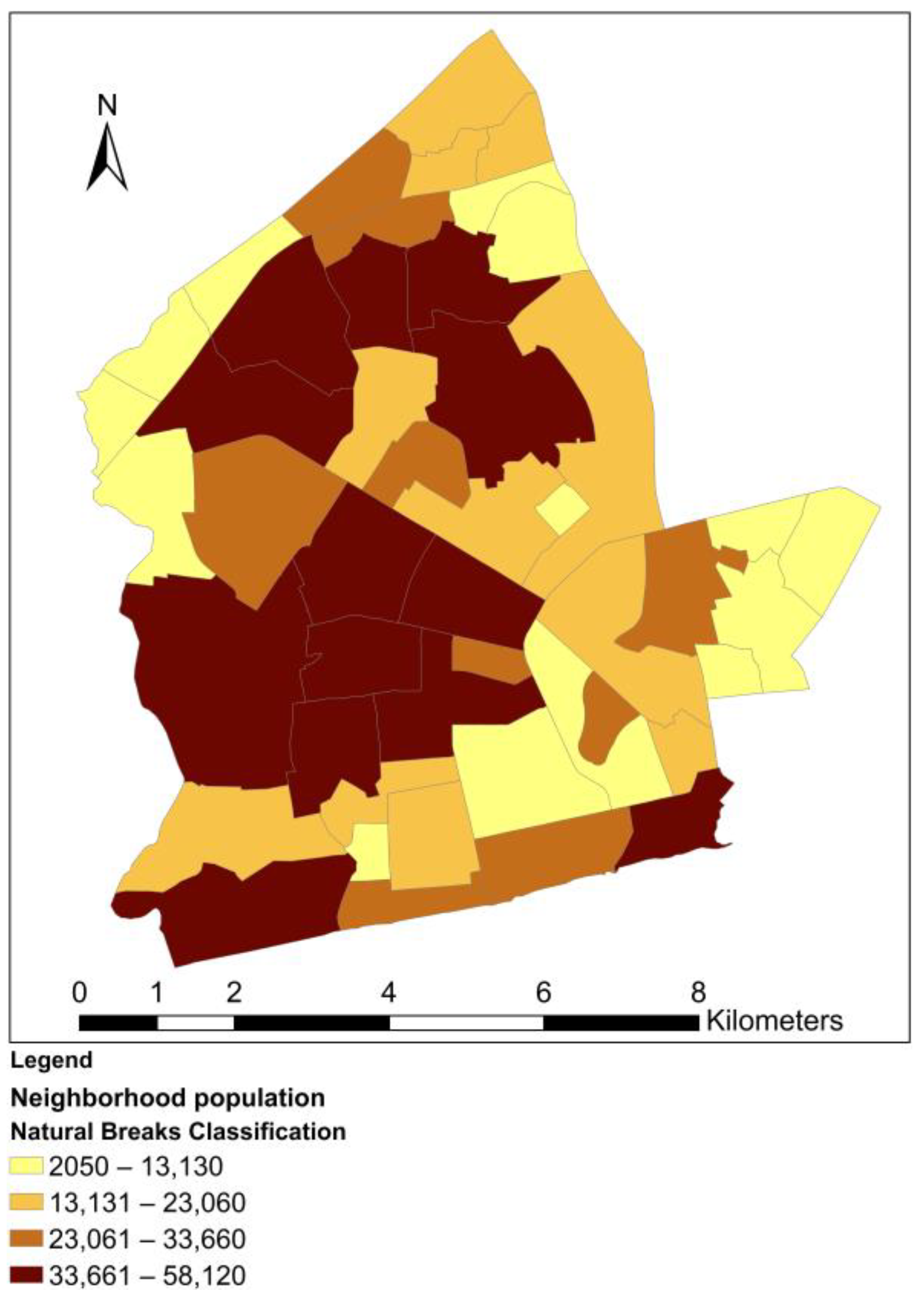
| Neighborhood population | number of people |
| Neighborhood population density | number of people per square kilometer |
| Load shedding exposure, | h |
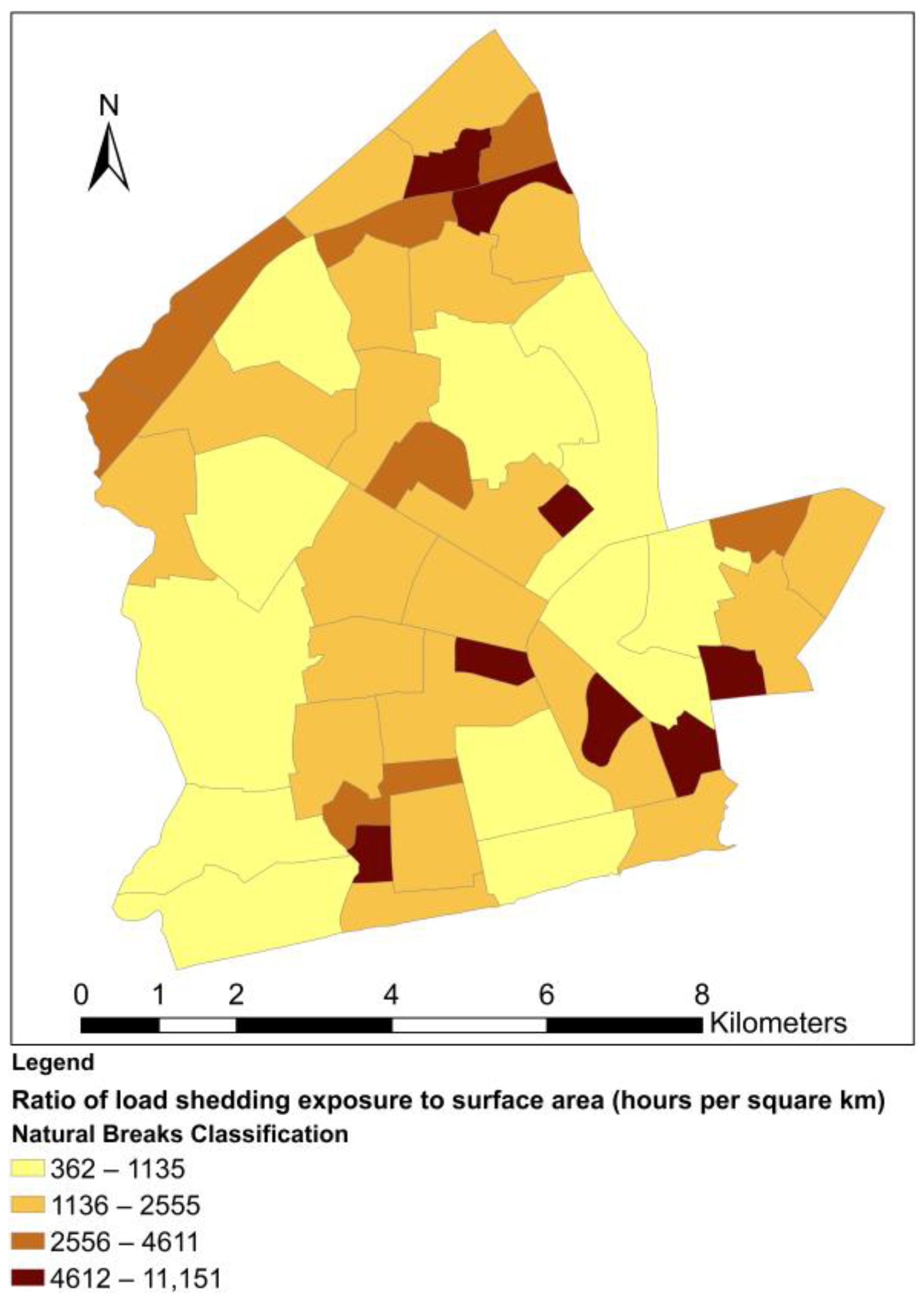
| h/km2 | |
| min/capita | |
| min/(capita/km2) |
| z-Score * | p-Value ** | Meaning | |
|---|---|---|---|
| Hot Spot | Cold Spot | ||
| >2.58 | <−2.58 | 0.01 | Statistically significant hot/cold spot at 99% confidence level |
| 1.96 to 2.58 | −2.58 to −1.96 | 0.05 | Statistically significant hot/cold spot at 95% confidence level |
| 1.65 to 1.96 | −1.96 to −1.65 | 0.1 | Statistically significant hot/cold spot at 90% confidence level |
| Cluster/Outlier Type | Explanation |
|---|---|
| High-High Cluster | Statistically significant * cluster with surrounding neighborhoods having similarly high outage values |
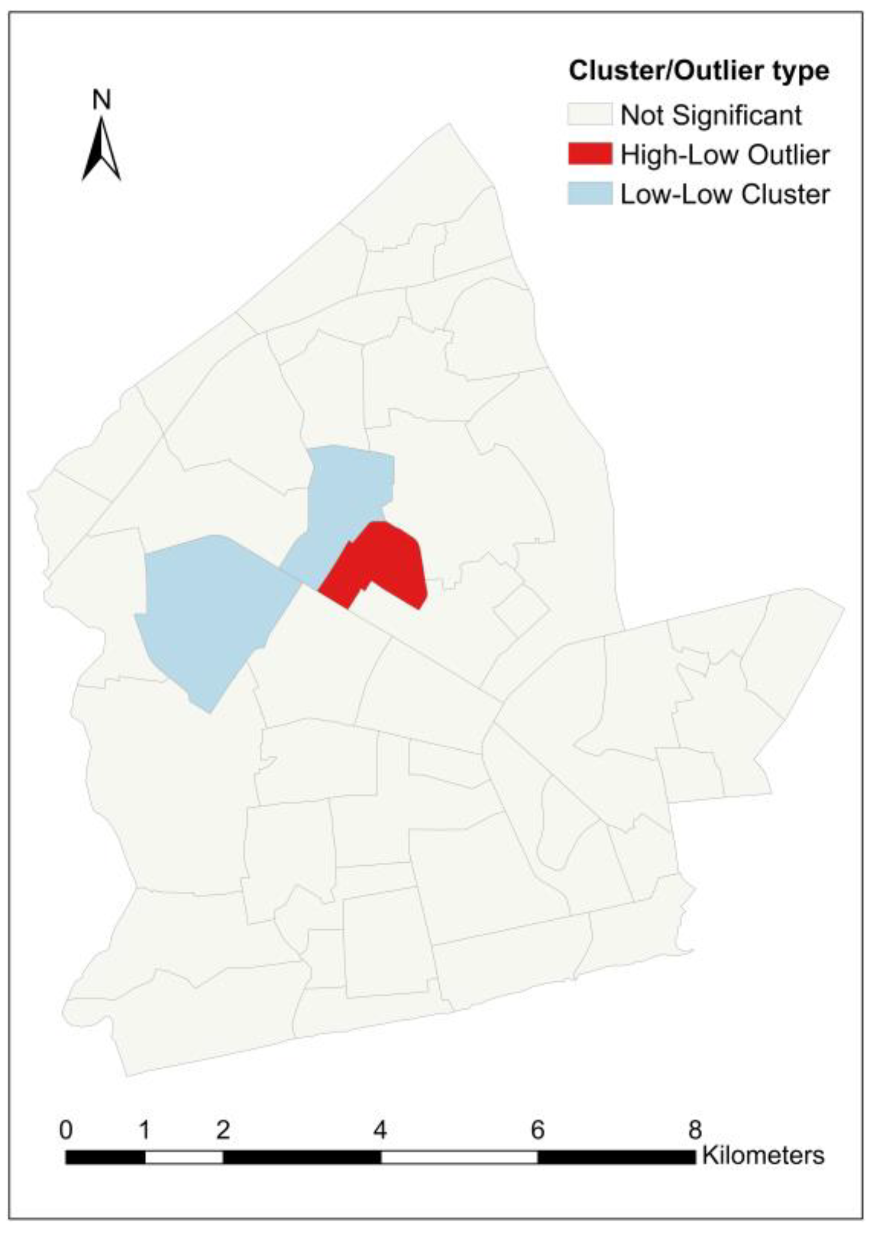
| High-Low Outlier | Statistically significant * spatial outlier with a high load-shedding exposure value surrounded primarily by neighborhoods with low load-shedding exposure values |
| Low-High Outlier | Statistically significant * spatial outlier with a low load-shedding exposure value surrounded primarily by neighborhoods with high load-shedding exposure values |
| Low-Low Cluster | Statistically significant * cluster with surrounding neighborhoods having similarly low outage values |
| Variable | Mean | Standard Deviation | Minimum | Maximum |
|---|---|---|---|---|
| Area (km2) | 1.48 | 0.96 | 0.26 | 5.12 |
| Neighborhood population | 24,505 | 14,860 | 2050 | 58,120 |
| Neighborhood population density | 19,930 | 13142 | 2443 | 65,838 |
| Load shedding exposure, (h) | 2497.40 | 549.81 | 1117 | 3244 |
| (h/km2) | 2632.17 | 2105.18 | 362 | 11,151 |
| (min/capita) | 11.11 | 13.66 | 1.54 | 84.59 |
| (min/capita/km2) | 11.96 | 10.56 | 2.60 | 64.79 |
| Variable | Moran’s I | z-Score | p-Value |
|---|---|---|---|
| Load shedding outage exposure, | 0.332901 | 3.841752 | 0.000122 ** |
| −0.086759 | −0.745002 | 0.456270 | |
| 0.092946 | 1.598783 | 0.109869 | |
| 0.181642 | 2.573218 | 0.010076 * |
| Hot Spot Analysis (Getis-Ord Gi* Statistic) | Cold Spots | Hot Spots | |
|---|---|---|---|
| Cold Spots | - | Adabraka | |
| Hot Spots | South Ordokor | - | |
| - | Asylum Down North Ridge Victoriaborg | ||
| Cluster and Outlier Analysis (Local Moran’s I Statistic) | Low-Low Cluster | High-High Cluster | |||
|---|---|---|---|---|---|
| Low-Low Cluster | - | Chorkor | - | - | |
| Darkuman | - | South Ordokor | - | ||
| - | New Fadama | Mataheko New Russia | - | ||
| High-High Cluster | - | - | - | North Ridge | |
| Hot Spot analysis (Gi* statistic). | Cluster and Outlier Analysis (Local Moran’s I Statistic) | ||||||
| Load Shedding Outage Exposure, | |||||||
| Load shedding outage exposure, | High-High Cluster | Low-Low Cluster | High-Low Outlier | Low-High Outlier | Insignificant | ||
| Hot Spot | Awoshie Dansoman Estate MatahekoNew Achimota New Russia South Ordokor Tsabaa | - | - | - | Achimota Akweteyman North Ordokor | ||
| Cold Spot | - | Chorkor KorleGonno Mamprobi Old Dansoman | - | - | Adabraka Gbegbeyise North Kaneshie North Industrial Area | ||
| Insignificant | - | Abeka | - | - | All the remaining neighbourhoods (28) | ||
| Hot Spot | - | - | - | - | - | ||
| Cold Spot | - | Darkuman South Ordokor | - | - | - | ||
| Insignificant | - | - | Bubiashie | - | All the remaining neighbourhoods (44) | ||
| Hot Spot | North Ridge | - | - | - | North Ridge Victoriaborg Asylum Down Awudome Estate | ||
| Cold Spot | - | - | - | - | - | ||
| Insignificant | - | New Russia Mataheko Darkuman New Fadama | Korle Lagoon Area | - | All the remaining neighbourhoods (38) | ||
| Hot Spot | North Ridge | - | - | Tudu Adabraka Asylum Down | Victoriaborg | ||
| Cold Spot | |||||||
| Insignificant | Chorkor Lapaz New Fadama | All the remaining neighbourhoods (39) | |||||
© 2020 by the authors. Licensee MDPI, Basel, Switzerland. This article is an open access article distributed under the terms and conditions of the Creative Commons Attribution (CC BY) license (http://creativecommons.org/licenses/by/4.0/).
Share and Cite
Nduhuura, P.; Garschagen, M.; Zerga, A. Mapping and Spatial Analysis of Electricity Load Shedding Experiences: A Case Study of Communities in Accra, Ghana. Energies 2020, 13, 4280. https://doi.org/10.3390/en13174280
Nduhuura P, Garschagen M, Zerga A. Mapping and Spatial Analysis of Electricity Load Shedding Experiences: A Case Study of Communities in Accra, Ghana. Energies. 2020; 13(17):4280. https://doi.org/10.3390/en13174280
Chicago/Turabian StyleNduhuura, Paul, Matthias Garschagen, and Abdellatif Zerga. 2020. "Mapping and Spatial Analysis of Electricity Load Shedding Experiences: A Case Study of Communities in Accra, Ghana" Energies 13, no. 17: 4280. https://doi.org/10.3390/en13174280
APA StyleNduhuura, P., Garschagen, M., & Zerga, A. (2020). Mapping and Spatial Analysis of Electricity Load Shedding Experiences: A Case Study of Communities in Accra, Ghana. Energies, 13(17), 4280. https://doi.org/10.3390/en13174280