Abstract
Short-term load forecasting (STLF) plays an important role in the economic dispatch of power systems. Obtaining accurate short-term load can greatly improve the safety and economy of a power grid operation. In recent years, a large number of short-term load forecasting methods have been proposed. However, how to select the optimal feature set and accurately predict multi-step ahead short-term load still faces huge challenges. In this paper, a hybrid feature selection method is proposed, an Improved Long Short-Term Memory network (ILSTM) is applied to predict multi-step ahead load. This method firstly takes the influence of temperature, humidity, dew point, and date type on the load into consideration. Furthermore, the maximum information coefficient is used for the preliminary screening of historical load, and Max-Relevance and Min-Redundancy (mRMR) is employed for further feature selection. Finally, the selected feature set is considered as input of the model to perform multi-step ahead short-term load prediction by the Improved Long Short-Term Memory network. In order to verify the performance of the proposed model, two categories of contrast methods are applied: (1) comparing the model with hybrid feature selection and the model which does not adopt hybrid feature selection; (2) comparing different models including Long Short-Term Memory network (LSTM), Gated Recurrent Unit (GRU), and Support Vector Regression (SVR) using hybrid feature selection. The result of the experiments, which were developed during four periods in the Hubei Province, China, show that hybrid feature selection can improve the prediction accuracy of the model, and the proposed model can accurately predict the multi-step ahead load.
1. Introduction
With the rapid development of the economy, the application of electricity in various aspects of production and living has been becoming increasingly widespread [1]. Faced with the difficulty of electrical energy storage, power plants need to generate electricity in accordance with the requirement of the power grid [2]. Short-term load forecasting (STLF) can provide a decision-making basis for generation dispatchers to draw up a reasonable generation dispatching plan [3], which plays a vital role in the optimal combination of units, economic dispatch, optimal power flow, and power market transactions [4]. However, the short-term load is sensitive to the external environment, such as climate change, date types, and social activities [5]. The randomness of the load sequence is raised by these uncertainties [6]. Therefore, how to identify the strong correlation factors of the extracted load from a host of influencing factors and realize the accurate prediction of the short-term load is an urgent problem to be solved in this research.
STLF has a dramatic impact on the external environment [7]. The load can be affected by various factors, such as temperature, weather, and date type [8]. When the temperature is in the extreme position, electrical appliances for heating or cooling will bring about the increase of the consumption of the load [9]. The type of date contributes to the change of the load by affecting the on-off state of the plant [10]. Therefore, extracting effective features from the uncertain influencing factors of load are able to lay the foundation for improving short-term load forecasting. Feature engineering refers to the selection of a representative subset of features in the feature set [11]. These features are highly correlated with the output variables and are the most common methods for extracting effective features. Common feature selection methods consist of autocorrelation (AC), mutual information (MI), ReliefF (RF), correlation-based feature selection (CFS), and so on [12]. Moon et al. used CFS to extract relevant features for rainfall prediction [13]. The feature subset selected by this method can shorten the training time of the model and reduce over-fitting. Yang et al. used the autocorrelation function (ACF) to select features and used Least Squares Support Vector Machines to predict the load [14]. The existing feature processing methods are formidable to ensure that the selected features are the optimal feature subsets [15]. Therefore, this study uses a hybrid feature extraction method to solve the above problems.
For the same load forecasting case, the upper limit of prediction accuracy differs among various features; for the same set of features, the performance of each prediction model is also different [16]. For decades, an ocean of advanced methods has been proposed to predict the power load [17]. The general prediction methods can be broadly divided into time series methods, machine learning methods, and deep learning methods [18]. Compared with traditional time series methods, these methods are relatively mature and there is no difficulty in implementing them [19]. These include autoregressive integrated moving average (ARIMA) [20], exponential smoothing [21], semi-parametric models (SPM) [22], multiple linear regression (MLR) [23], and so on. However, they are all based on linear analysis and unable to accurately describe the specific trend of STLF [24].
As the research of machine learning is becoming a hot spot nowadays, these methods have been applied to various prediction fields. Liu et al. put forward a runoff prediction method which combines hidden Markov and Gaussian process regression [25]. Liu et al. proposes an ultra-short-time forecasting method based on the Takagi–Sugeno (T–S) fuzzy model for wind power and wind speed. This method employs meteorological measurements as input and can get accurate prediction results [26]. Machine learning also has a pleasurable effect on STLF [27]. Khwaja et al. presented an artificial neural network (ANN) and ensemble machine learning to improve short-term load prediction [18]. Compared with traditional models, such as traditional exponential smoothing (ARMA), it performs higher accuracy.
With the increasing development of artificial intelligence, a multitude of traditional machine learning methods are unable to catch up with deep learning methods [28]. A high number of improved deep learning models have also appeared one after another, and these models are applied to various fields for predicting. Tao et al. developed the convolutional-based bidirectional gated recurrent unit (CBGRU) method to forecast air pollution [29]. Liu et al. proposed the experimental Bayesian deep learning model to predict the wind speed with good accuracy [30]. Similarly, deep learning showed significant achievements in STLF [31]. Guo et al. developed Multilayer Perceptron (MLP) and Quantile Regression (QR) for point prediction and probabilistic prediction of the short-term load [32]. The model has a better forecasting accuracy in terms of measuring electricity consumption relative to the random forest and gradient boosting model.
The prediction of time series by recurrent neural networks (RNN) has been adopted by more and more people [33]. However, when RNN works out the long-term dependence problem, it would face problems of gradient disappearance and gradient explosion [34]. To solve such problems, the Long Short Memory Network (LSTM) was proposed by Hochreiter and Schmidhuber in 1997 [35]. The concepts of gate, input gate, output gate, and forget gate were proposed for the application of the network. After years of testing, LSTM showed a more prominent contribution in timing prediction than RNN. In recent years, numerous LSTM variants have been proposed. Zhang et al. unified the gates in the LSTM network into one gate, and these gates share the same set of weights, thereby reducing training time [36]. Pei et al. changed the structure in the LSTM network to achieve better prediction results and shorter training time [37]. These variants of LSTM are well applied to short-term prediction.
Nowadays, most of the researches focus on single-step STLF. However, accurate multi-step STLF has a more important significance for formulating generation scheduling plans [38]. It can formulate longer-term plans for electric power dispatching, and reap greater benefits for electric power operators [39]. This paper is devoted to the exploration of multi-step STLF. In order to test the limit prediction ability of the model under the requirement of short-term load prediction accuracy, the model is proposed to predict multi-step prediction of the power load in the Hubei Province. This study provides technical support for a power system to formulate a generation plan.
Compared with the existing research of short-term load forecasting, the highlights and advantages of our study are as follows:
(1) The model not only considers other influencing factors such as the environment on short-term load forecasting, but also pays more attention to the influence of the historical load on the model and adopts a two-stage feature selection method to select load features of 168 time periods from the previous week;
(2) This paper proposes an Improved Long Short-Term Memory network for load prediction. This network changes the characteristics of the original door and the transfer method of the cell. Compared with the traditional LSTM, it has higher prediction accuracy;
(3) Most of the popular short-term load forecasting models predict the load of the next period (hour-ahead or day-ahead). This article is dedicated to studying the load of the next multi-period (multi-step ahead). This is more conducive to rationally arrange the power generation tasks of the power station and ensure the stability of the power system operation. This research has more practical significance.
2. Methodology
In this section, the method of feature selection used in this paper is first introduced. This method is composed of the filter feature selection method and wrapper feature selection method. The specific step and formula are shown in Section 2.1. The main predictive model, the Improved Long Short-Term Memory network [37], is introduced in Section 2.2. Furthermore, the overall steps of the predictive model and its flow chart are shown in Section 2.3.
2.1. Hybrid Feature Selection
In the study of load forecasting, there are plenty of influencing factors that affect it, such as the previous load, the date type, temperature, dew point, and humidity. Establishing an accurate load forecasting model should be combined with environmental factors and date types. When the temperature is higher, the operating power of the refrigeration equipment will be greatly increased, and it would directly affect the power load. When the temperature is lower, the opening of the heating equipment would also have an impact. When it comes to holidays, the load impact of factory shutdowns is also huge. Therefore, quantitative analysis of these factors is important for load changes.
For non-numeric features, such as date types, they should be quantified. The date types selected in this article are workdays, rest days, and holidays. Such non-numeric features need to be encoded. The maximum number of days for Chinese holidays is 7 days, so they can be mapped to the code as shown in Table 1. Holiday1 represents a holiday for one day, and so on. Other numerical features are normalized accordingly.

Table 1.
Mapping encoding for date type.
The effect of these factors above is complex. The maximal information coefficient (MIC) is applied to measure the nonlinear dependence between factors and power load. The closer MIC is to 1, the stronger the nonlinear dependence. The formula of MIC is given as follows:
where represents the mutual information coefficient between and . is the joint probability density of variable and , and and are the marginal probability densities of variables and , respectively.
Peng et al. proposed a feature selection method named Max-Relevance and Min-Redundancy [40] that could use mutual information scores to select features. The purpose is to punish the correlation of features by their redundancy in the presence of other selected features. The correlation of feature set with class is defined by the average of all mutual information values between each feature and class , as follows:
The redundancy of all features in set is the mean value of all mutual information values between feature and feature :
Combined with the constraints of the above two formulas, a parameter is defined to optimize and simultaneously.
In practice, incremental search methods can be used to obtain near-optimal features. The formula is as follows:
where represents the set of all features. represents the selected feature subset, and its feature subset contains features. This method is based on the selected features to find the feature that maximizes the value of the above formula in the remaining feature space. In fact, each of the remaining features is calculated and then sorted. Therefore, the essence of this method is to use a standard (correlation–redundancy) to sort the features, but we need to select a feature subset firstly, then it can be calculated. The search method is a first-order incremental search. This method can only sort the remaining feature sets. It is better to put the first feature in the remaining feature set into the feature subset rather than the later feature, but it cannot guarantee that the prediction accuracy after adding the feature is better than before. In this paper, the load features are preliminarily screened by MIC as a feature subset, and then the remaining features are sorted by the mRMR method. Add the first feature in the remaining feature set in the feature subset and put them into the model for prediction. If the accuracy is improved, continue this process until the accuracy becomes lower.
2.2. Improved Long Short-Term Memory Network
LSTM was first proposed by Sepp Hochreiter and Schmidhuber in 1997 [35]. It is an advanced version of Recurrent Neural Network (RNN). Compared with RNN, its essence lies in the introduction of the concept of the cell state. The cell state of LSTM will determine which states should be left behind and which states should be forgotten. The problem of the disappearance of the RNN gradient has been solved. The LSTM network has three gates in the hidden layer (input gates, output gates, and forget gates). Input gates control the input flow of the memory cell, and output gates control the output flow into other cells. The role of forget gates is to selectively forget the information in the state of the cell. The traditional LSTM network has a longer training time due to the complex structure. In order to achieve the purpose of reducing network training time without affecting accuracy, the structure of LSTM is improved, and the Improved Long Short-Term Memory Network (ILSTM) is proposed. ILSTM combines input gates and forget gates into one new gate to reduce network complexity. The structure of ILSTM network is shown in Figure 1. The forward propagation and formula of ILSTM in the t-th period are elaborated as follows.
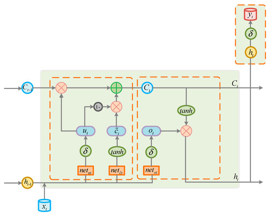
Figure 1.
Schematic diagram of the Improved Long Short-Term Memory (ILSTM) network structure.
Calculate shared gates
Calculate current information state
Update cell memory
Calculate output gates
Calculate output of hidden layer
Calculate output of predicted value
In the above formula, , , , and are the state of the current stage. , , and are their weight matrices. , , and represent the bias vectors. , , , and are the input of input layer, the shared gates, the information state, and output gates in the current period, respectively. and represent the cell state in the previous period and current period. The symbol is the multiplication of the matrix, and the symbol is the multiplication between the elements in the matrix. is the activation function of Sigmoid(), and is the activation function of and Tanh(). Their calculated formula is elaborated as follows:
Compared with LSTM, ILSTM cuts back the number of doors, reducing the variables needed to be optimized in the weight matrix. In the way of memory cell update, ILSTM first activates the current information state by using the activation function Tanh(). Next, it makes a linear combination of the previous cell memory and current information state , using update gate as the weight of the current information state and as the weight of the previous cell memory . The sum of the two weights is equal to one. In this way, cell memory is updated.
2.3. The Framework of the Proposed Model
In the entire prediction model, the features are first preprocessed. Since the power load changes periodically, the feature can be selected by referring to the period. The period of load change can be regarded as one week, so the hourly power load (168 in total) within seven days is selected as the preliminary feature of past load in this paper. First, we calculated MIC separately between the load of this period and the load of the previous 168 periods . Features (MIC > 0.6) were placed in the temporary feature subset, and features (MIC < 0.6) were placed in the candidate feature subset. Next, the root mean square error (RMSE) was used to discriminate the prediction effect. The mRMR method was adopted to select features under candidate subset and to add them to the feature subsets until the prediction accuracy becomes low. The selected load features, environment features, and date features were integrated to obtain the final feature set together and put into the ILSTM network for training. The prediction models were established for single step prediction, two-step prediction, three-step prediction, and multi-step prediction, respectively. The complete framework of the model is shown in Figure 2, and the Schematic diagram of multi-step prediction is shown in Figure 3.
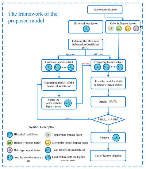
Figure 2.
The framework of the proposed model.
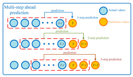
Figure 3.
Schematic diagram of multi-step prediction.
3. Evaluation Criteria
In this paper, four indicators, including RMSE (Root Mean Square Error), MAE (Mean Absolute Error), MAPE (Mean Absolute Percentage Error), and (coefficient of determination) are adopted to evaluate the prediction accuracy of the model. Specific formulas for each indicator are listed as shown in Table 2.
Table 2.
Specific instruction for each indicator.
is the size of the test sample and refers to the i-th predicted value. refers to the i-th observed value and is the mean of observed value. The smaller the final MAE, MAPE, and RMSE, the higher the prediction accuracy. The closer is to 1, the higher the prediction accuracy.
In order to further evaluate the accuracy between the two different models, three indicators, , , and , are applied. The specific formula is as follows:
In order to better evaluate the future operational risks generated by model predictions, we used the standard deviation of the error as a criterion. The specific formula is as follows:
4. Case Study
In this section, we first introduce the basic data for the power load and the corresponding factors applied to the model. In order to verify that the proposed model has high-precision prediction results, four datasets are used for testing and compared with existing popular models. In addition, multiple predictive period experiments further confirm the practicability of the model. In the predictive model, all deep learning models are implemented using the keras framework, and SVR is implemented using the “sklearn” framework in python.
4.1. Data Introduction
In this case, the power load and related influencing factors are first introduced. The data used in this paper comes from the Huazhong Power Grid Corporation, which is the hourly load data for 2015 from the Hubei Province, China. In this year, the average annual temperature in Hubei was about 18 degrees. January and February were the coldest times of the year. The minimum temperature reached numbers below zero. The temperature became higher in July and August, and the highest temperature reached 40 degrees and more. The power load in January and February was higher than the annual average due to the application of heating equipment. From March to June, the temperature has been stable below the average. In the summer, the large-scale application of the refrigeration system seriously affected the power load. During this period, the power load was the highest in the whole year. With the weather turned cooler from September to November, the load weakened accordingly until the temperature began to rise steadily. The lowest power load of the year was the Spring Festival due to factory holidays. The annual electrical load data and environmental data are shown in Figure 4.
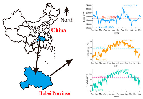
Figure 4.
Environmental variables and load in the Hubei Province.
In order to better evaluate the performance of the model, the load data is divided into four datasets according to the quarter. It can be seen from the figure that the first dataset shows a large fluctuation range, the second dataset is relatively stable, the third dataset performs a high peak value, and the power load in the fourth dataset drops sharply and then slowly rises. According to this classification, the dataset can be better trained and is representative. The detailed parameters of the dataset are shown in Table 3.
Table 3.
Specific information of four datasets.
In this paper, the data of the missing period is obtained by using the average value of the load of the previous period and the load of the next period. The first 80% of the original dataset is used as training data to train the model, and the other 20% is used as test data. The models are trained using the cross-validation [41,42]. Tr, Te represents the number of training sets and test sets, respectively. Sum represents the total number of datasets. Four datasets are shown in Figure 5.
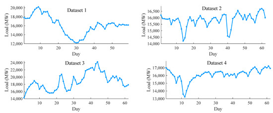
Figure 5.
The daily average load for four datasets.
4.2. Feature Combination Selection
In the proposed method, the original load characteristics are pre-processed. Firstly, the load characteristics of the dataset in the first seven days (168 time periods) are calculated for the maximum information coefficient of the current period, and the features with a MIC value greater than 0.6 are selected. The MIC value of the load of the first 168 periods and the current period load in dataset 1 to dataset 4 are shown in Figure 6, Figure 7, Figure 8 and Figure 9.
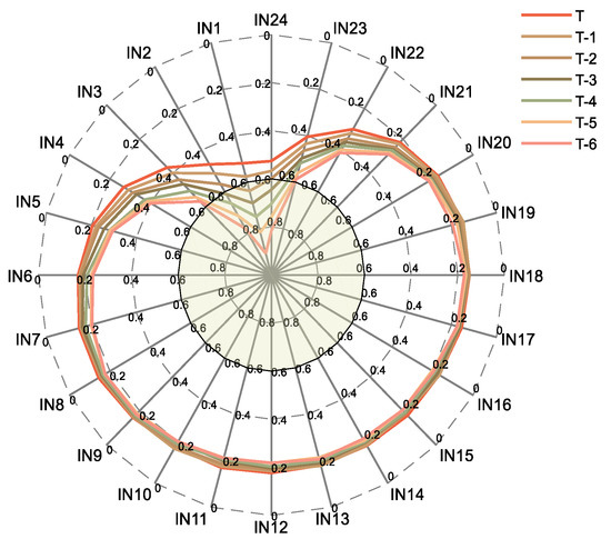
Figure 6.
Maximal information coefficient (MIC) of historical load for dataset 1.
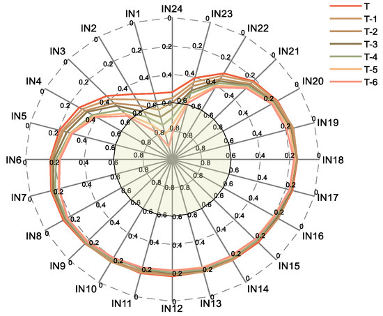
Figure 7.
MIC of historical load for dataset 2.
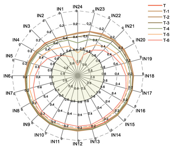
Figure 8.
MIC of historical load for dataset 3.
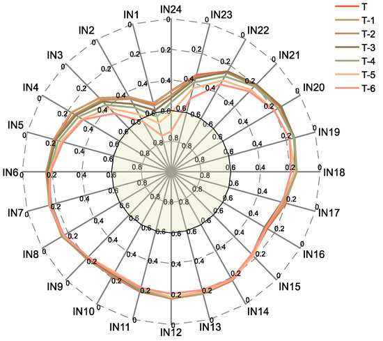
Figure 9.
MIC of historical load for dataset 4.
T represents the period of the day when the load is to be predicted, T-1 represents the day before the predicted load, IN1 represents the current load in the past hour, IN2 represents the current load for the past two hours, and so on.
After the preliminary screening of features, make a second selection of the remaining feature. The features including the environment features and the encoded date features are added to the feature subset, and the features of the candidate subset are sorted by the mRMR method. The first ranked feature is placed in the feature subset for training. If the prediction accuracy becomes higher, the feature is retained, and continue the above process. If the accuracy becomes lower, stop the selection. The selected feature tables under the four datasets are shown in Table 4, where t-n represents the load characteristics of the previous n hours predicted at that time. The final feature set is used by the model to make predictions.
Table 4.
The final feature selection result of four datasets.
4.3. Parameter Settings
To validate the performance of the model, other popular models (LSTM, GRU, SVR) are used for comparison. In order to achieve fairness, the parameters of different models should be chosen as much as possible. The parameters selected in this article are all optimized with GA or some common values. For the purpose of eliminating the error caused by randomness, each model is run multiple times to average the results. The specific parameters are as shown in Table 5:
Table 5.
Parameter details of deep learning models.
4.4. Experiment Results and Discussion
In this section, the current popular models are compared with the proposed method to predict the short-term load. The results of various models under the 1-step, 2-step, and 3-step load forecasting will be introduced as follows, and MAE, MAPE, RMSE, and R2 are used to evaluate the accuracy of the model. Cpu times of the algorithms (CT) is used to indicate the time required for model calculation, and S is used to evaluate the future operational risks generated by model predictions
(1) The analysis of the one-step prediction
The prediction results of each model on the dataset are shown in Table 6. H-ILSTM represents the model combined with hybrid feature selection and ILSTM. The detailed index comparison figure for dataset 1 is shown in Figure 10 and Figure 11. The figure shows the load forecast results of 96 time periods in the test set for dataset 1. The bold words in the table represent the best prediction results among the eight models. It can be clearly seen that the hybrid feature selection method has improved the model to varying degrees in every dataset. Among them, the H-ILSTM model has the highest prediction accuracy, and the value of the standard deviation of the prediction error is also the smallest. Compared with the model which does not adopt a hybrid feature selection method, the specific improvement effect of this model is shown in Table 7. The forecast accuracy improved by nearly 50%.
Table 6.
One-step prediction result of load. (The bold words in the table represent the best prediction results among the eight models).
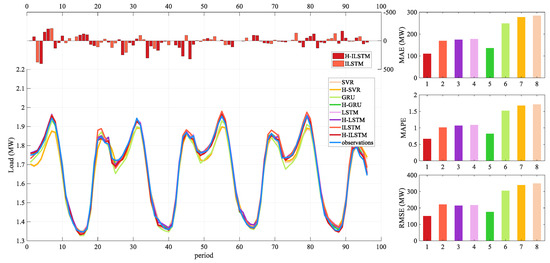
Figure 10.
Forecasting performance of eight models for dataset 1.
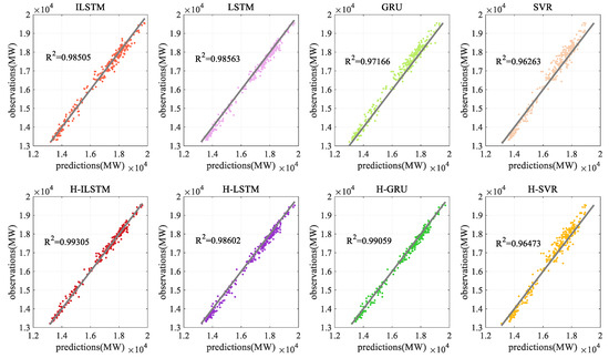
Figure 11.
Coefficient of determination by different methods for dataset 1.
Table 7.
The promoting percentages of the ILSTM model by the H-ILSTM model of one-step prediction for the load datasets 1–4.
Compared with the recently popular model, H-ILSTM is also very competitive. As shown in Table 8, the accuracy of this model is compared with other prediction models. The evaluation index is the average of the four datasets. H-ILSTM has a better prediction effect than the original LSTM network, and the prediction accuracy is improved by about 20%. Compared with machine learning, the prediction accuracy has been significantly improved.
Table 8.
The promoting percentages of the other models by the H-ILSTM model of one-step prediction for the load datasets 1–4.
(2) The analysis of the two-step prediction
The prediction accuracy is reduced compared to the one-step prediction, but the model still maintains a high accuracy. The two-step prediction results of various models under four data are shown in Table 9. The bold characters in the table represent the best predictions among the eight models. The comparison figure of forecast indicators is shown in Figure 12 and Figure 13. The figure shows the load forecast results of 96 time periods in the test set for dataset 2. Among them, H-ILSTM predicted the best performance under the four datasets.
Table 9.
The two-step prediction result of the load. (The bold characters in the table represent the best predictions among the eight models).
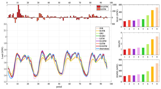
Figure 12.
The use of hybrid feature selection has greatly improved the model prediction, and the relative value of each prediction evaluation index of the ILSTM model is shown in Table 10. Compared with not using the hybrid feature selection method, the average Mean Absolute Error (MAE) predicted by this method is improved by 23.8, Mean Absolute Percentage Error (MAPE) is improved by 21.6, and Root Mean Square Error (RMSE) is improved by 23.9. Based on this, it shows that this feature extraction method plays an important role in two-step prediction.
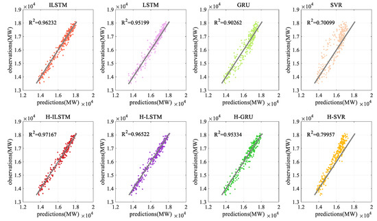
Figure 13.
Coefficient of determination by different methods for dataset 2.
Compared with other models, the H-ILSTM model has improved to varying degrees under the four datasets. The improvement indicators are shown in Table 11.
Table 11.
The promoting percentages of the other models by the H-ILSTM model of the two-step prediction for the load datasets 1–4.
(3) The analysis of the three-step prediction
The model can still maintain a relatively high prediction accuracy. The three-step prediction results of various models under four data are shown in Table 12. The bold characters in the table represent the best predictions among the eight models. The comparison figure of forecast indicators is shown in Figure 14 and Figure 15. The figure shows the load forecast results of 96 time periods in the test set for dataset 4.
Table 12.
The three-step prediction result of the load. (The bold characters in the table represent the best predictions among the eight models).
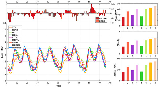
Figure 14.
Forecasting performance of eight models for dataset 4.
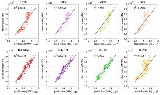
Figure 15.
Coefficient of determination by different methods for dataset 4.
The use of the hybrid feature selection method has slightly improved the ILSTM model, and each forecast evaluation index has been improved by more than 20%. The details are shown in Table 13.
Table 13.
The promoting percentages of the ILSTM model by the H-ILSTM model of the three-step prediction for the load datasets 1–4.
Compared with other models, the average value of each evaluation index under the four datasets has increased by about 15%. The details are shown in Table 14.
Table 14.
The promoting percentages of the other models by the H-ILSTM model of the three-step prediction for the load datasets 1–4.
(4) The analysis of the multi-step prediction
This section mainly tests the limit prediction ability of the H-LSTM model proposed in this paper. Make predictions of multi-step for four datasets, respectively, and establish prediction thresholds. If the prediction accuracy is less than this threshold, the prediction is stopped. This threshold is evaluated using the decision coefficient R2. The result is shown in Figure 16.
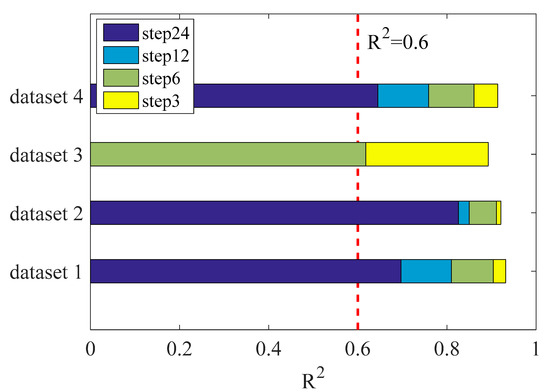
Figure 16.
Coefficient of determination for the multi-step prediction under four datasets.
It can be seen from the figure that the model performs best under dataset 2 and can accurately predict the load in the next 24 h. In dataset 1 and dataset 4, the model can more accurately predict the load for the next 24 periods. The performance in dataset 3 is general and can only be predicted for the next 6 h. Due to the large fluctuations in the peaks, the model has a slightly insufficient ability to predict such multi-steps. Compared with dataset 1, dataset 2, and dataset 4, the model has a good prediction performance for such datasets. Both can accurately predict the load in the next 6 h, and thus can more accurately predict the load in the next 24 h. The model also has room for improvement under load datasets with large fluctuations
(5) Comparison experiment between the proposed model and the persistence model
A good baseline for time series forecasting is the persistence model. This is a predictive model in which the last observation is persisted forward. This method uses the “today equals tomorrow” concept [43]. In order to better evaluate the effect of the proposed method, we conducted a test comparison between the proposed method and the persistence model, and used MAE, MAPE, RMSE, and R2 for evaluation. This section shows the experiment of single-step prediction in dataset 1. Figure 17 shows the prediction effects of the two models. The evaluation indicators are listed in Table 15. In terms of indicators, the persistence model is close to the proposed model on R2. All other indicators are worse than the proposed model.
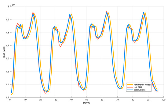
Figure 17.
Forecasting performance of two models for dataset 1.
Table 15.
Evaluation criteria for single-step prediction under dataset 1.
5. Conclusions
STLF has a very important leading role in the power grid. In order to improve the accuracy of short-term load forecasting, this paper first starts from feature engineering, taking into account the relevant factors that affect the load, such as weather conditions and date types, and the hybrid feature selection is adopted. The improved LSTM network is used for multi-step prediction. The datasets of four time periods in the Hubei Province are selected and compared with the LSTM, GRU, and SVR models using the hybrid feature selection method. The effects of model prediction are reflected through MAE, RMSE, MAPE, and R2. , , and are used to reflect the difference of prediction results between models. From the experimental results, the prediction accuracy of the ILSTM model using the hybrid feature selection method is higher than the ILSTM model without this method in four datasets on average by more than 20%. The accuracy of the H-ILSTM model is about 15% higher than that of other models using the hybrid feature selection method. We also tested the multi-step prediction ability of the proposed model, which has a satisfactory performance. To sum up the following conclusions:
- (1)
- The hybrid feature selection method can improve the prediction accuracy of the model;
- (2)
- The ILSTM model is better than other traditional forecasting models in short-term load forecasting;
- (3)
- The H-ILSTM model has a good prediction effect in multi-step prediction.
Therefore, the proposed method has a very eye-catching performance in short-term multi-step load forecasting, which can more accurately predict the load in the next few periods. This model is competitive in this field.
The proposed model also has some shortcomings. When selecting features, it only considers the optimal combination of historical loads. Other influencing factors are just normalized as one of the inputs of the model. Secondly, it takes a lot of time to select features. We will gradually improve these issues in future research.
Author Contributions
Conceptualization, S.P. and H.Q.; methodology, S.P.; software, L.Y.; validation, H.Q., S.P.; formal analysis, S.P.; investigation, S.P.; resources, H.Q. and Y.L.; data curation, C.W.; writing—original draft preparation, S.P.; writing—review and editing, Y.L. and H.Q.; visualization, S.P.; supervision, J.Z.; project administration, H.Q.; funding acquisition, H.Q. All authors have read and agreed to the published version of the manuscript.
Funding
This research was funded by the Open Research Fund of State Key Laboratory of Simulation and Regulation of Water Cycle in River Basin (China Institute of Water Resources and Hydropower Research, grant number: No. IWHR-SKL-KF201914), National Natural Science Foundation of China (grant number: No. 51979113, U1865202), National Public Research Institutes for Basic R & D Operating Expenses Special Project (grant number: CKSF2017061/SZ). The APC was funded by National Natural Science Foundation of China (grant number: No. 51979113).
Conflicts of Interest
The authors declare no conflict of interest.
References
- Santos, P.J.; Martins, A.G.; Pires, A.J.; Martins, J.F.; Mendes, R.V. Short-term load forecast using trend information and process reconstruction. Int. J. Energ. Res. 2006, 30, 811–822. [Google Scholar] [CrossRef]
- Zhai, M. A new method for short-term load forecasting based on fractal interpretation and wavelet analysis. Int. J. Elec. Power 2015, 69, 241–245. [Google Scholar] [CrossRef]
- Cai, Q.; Yan, B.; Su, B.; Liu, S.; Xiang, M.; Wen, Y.; Cheng, Y.; Feng, N. Short-term load forecasting method based on deep neural network with sample weights. Int. Trans. Electr. Energy Syst. 2020, 30. [Google Scholar] [CrossRef]
- Abedinia, O.; Amjady, N. Short-term load forecast of electrical power system by radial basis function neural network and new stochastic search algorithm. Int. Trans. Electr. Energy 2016, 26, 1511–1525. [Google Scholar] [CrossRef]
- Sadaei, H.J.; Guimarães, F.G.; José Da Silva, C.; Lee, M.H.; Eslami, T. Short-term load forecasting method based on fuzzy time series, seasonality and long memory process. Int. J. Approx. Reason. 2017, 83, 196–217. [Google Scholar] [CrossRef]
- El-Hendawi, M.; Wang, Z. An ensemble method of full wavelet packet transform and neural network for short term electrical load forecasting. Electr. Power Syst. Res. 2020, 182, 106265. [Google Scholar] [CrossRef]
- Liu, Y.; Lei, S.; Sun, C.; Zhou, Q.; Ren, H. A multivariate forecasting method for short-term load using chaotic features and RBF neural network. Eur. Trans. Electr. Power 2011, 21, 1376–1391. [Google Scholar] [CrossRef]
- Karimi, M.; Karami, H.; Gholami, M.; Khatibzadehazad, H.; Moslemi, N. Priority index considering temperature and date proximity for selection of similar days in knowledge-based short term load forecasting method. Energy 2018, 144, 928–940. [Google Scholar] [CrossRef]
- Rahman, S. Formulation and analysis of a rule-based short-term load forecasting algorithm. IEEE 1990, 78, 805–816. [Google Scholar] [CrossRef]
- He, F.; Zhou, J.; Feng, Z.; Liu, G.; Yang, Y. A hybrid short-term load forecasting model based on variational mode decomposition and long short-term memory networks considering relevant factors with Bayesian optimization algorithm. Appl. Energ. 2019, 237, 103–116. [Google Scholar] [CrossRef]
- Koprinska, I.; Rana, M.; Agelidis, V.G. Correlation and instance based feature selection for electricity load forecasting. Knowl.-Based Syst. 2015, 82, 29–40. [Google Scholar] [CrossRef]
- Kong, X.; Li, C.; Wang, C.; Zhang, Y.; Zhang, J. Short-term electrical load forecasting based on error correction using dynamic mode decomposition. Appl. Energ. 2020, 261, 114368. [Google Scholar] [CrossRef]
- Moon, S.; Kim, Y. An improved forecast of precipitation type using correlation-based feature selection and multinomial logistic regression. Atmos. Res. 2020, 240, 104928. [Google Scholar] [CrossRef]
- Yang, A.; Li, W.; Yang, X. Short-term electricity load forecasting based on feature selection and Least Squares Support Vector Machines. Knowl.-Based Syst. 2019, 163, 159–173. [Google Scholar] [CrossRef]
- Leung, Y.; Hung, Y. A Multiple-Filter-Multiple-Wrapper Approach to Gene Selection and Microarray Data Classification. IEEE/ACM Trans. Comput. Biol. Bioinform. 2010, 7, 108–117. [Google Scholar] [CrossRef]
- Zhang, Z.; Qin, H.; Liu, Y.; Yao, L.; Yu, X.; Lu, J.; Jiang, Z.; Feng, Z. Wind speed forecasting based on Quantile Regression Minimal Gated Memory Network and Kernel Density Estimation. Energ. Convers. Manag. 2019, 196, 1395–1409. [Google Scholar] [CrossRef]
- Zhang, W.; Mu, G.; Yan, G.; An, J. A power load forecast approach based on spatial-temporal clustering of load data. Concurr. Comput. Pract. Exp. 2018, 30, e4386. [Google Scholar] [CrossRef]
- Khwaja, A.S.; Anpalagan, A.; Naeem, M.; Venkatesh, B. Joint bagged-boosted artificial neural networks: Using ensemble machine learning to improve short-term electricity load forecasting. Electr. Power Syst. Res. 2020, 179, 106080. [Google Scholar] [CrossRef]
- Mohan, N.; Soman, K.P.; Sachin Kumar, S. A data-driven strategy for short-term electric load forecasting using dynamic mode decomposition model. Appl. Energ. 2018, 232, 229–244. [Google Scholar] [CrossRef]
- De Felice, M.; Alessandri, A.; Catalano, F. Seasonal climate forecasts for medium-term electricity demand forecasting. Appl. Energ. 2015, 137, 435–444. [Google Scholar] [CrossRef]
- Christiaanse, W. Short-Term Load Forecasting Using General Exponential Smoothing. IEEE Trans. Power Appar. Syst. 1971, 900–911. [Google Scholar] [CrossRef]
- Goude, Y.; Nedellec, R.; Kong, N. Local Short and Middle Term Electricity Load Forecasting With Semi-Parametric Additive Models. IEEE Trans. Smart Grid. 2014, 5, 440–446. [Google Scholar] [CrossRef]
- Saber, A.Y.; Rezaul Alam, A.K.M. Short Term Load Forecasting Using Multiple Linear Regression for Big Data, 2017; IEEE: Honolulu, HI, USA, 2017; pp. 1–6. [Google Scholar]
- Nie, H.; Liu, G.; Liu, X.; Wang, Y. Hybrid of ARIMA and SVMs for Short-Term Load Forecasting. Energy Procedia 2012, 16, 1455–1460. [Google Scholar] [CrossRef]
- Liu, Y.; Ye, L.; Qin, H.; Hong, X.; Ye, J.; Yin, X. Monthly streamflow forecasting based on hidden Markov model and Gaussian Mixture Regression. J. Hydrol. Amst. 2018, 561, 146–159. [Google Scholar] [CrossRef]
- Liu, F.; Li, R.; Dreglea, A. Wind Speed and Power Ultra Short-Term Robust Forecasting Based on Takagi–Sugeno Fuzzy Model. Energies 2019, 12, 3551. [Google Scholar] [CrossRef]
- Zeng, N.; Zhang, H.; Liu, W.; Liang, J.; Alsaadi, F.E. A switching delayed PSO optimized extreme learning machine for short-term load forecasting. Neurocomputing 2017, 240, 175–182. [Google Scholar] [CrossRef]
- Wang, H.; Lei, Z.; Zhang, X.; Zhou, B.; Peng, J. A review of deep learning for renewable energy forecasting. Energ. Convers. Manag. 2019, 198, 111799. [Google Scholar] [CrossRef]
- Tao, Q.; Liu, F.; Li, Y.; Sidorov, D. Air Pollution Forecasting Using a Deep Learning Model Based on 1D Convnets and Bidirectional GRU. IEEE Access 2019, 7, 76690–76698. [Google Scholar] [CrossRef]
- Liu, Y.; Qin, H.; Zhang, Z.; Pei, S.; Jiang, Z.; Feng, Z.; Zhou, J. Probabilistic spatiotemporal wind speed forecasting based on a variational Bayesian deep learning model. Appl. Energ. 2020, 260, 114259. [Google Scholar] [CrossRef]
- Tong, C.; Li, J.; Lang, C.; Kong, F.; Niu, J.; Rodrigues, J.J.P.C. An efficient deep model for day-ahead electricity load forecasting with stacked denoising auto-encoders. J. Parallel Distrib. Comput. 2018, 117, 267–273. [Google Scholar] [CrossRef]
- Guo, Z.; Zhou, K.; Zhang, X.; Yang, S. A deep learning model for short-term power load and probability density forecasting. Energy 2018, 160, 1186–1200. [Google Scholar] [CrossRef]
- Schuster, M.; Paliwal, K.K. Bidirectional recurrent neural networks. IEEE Trans. Signal Process. 1997, 45, 2673–2681. [Google Scholar] [CrossRef]
- Yamada, T.; Murata, S.; Arie, H.; Ogata, T. Representation Learning of Logic Words by an RNN: From Word Sequences to Robot Actions. Front Neurorobot. 2017, 11, 70. [Google Scholar] [CrossRef] [PubMed]
- Hochreiter, S.; Schmidhuber, J. Long Short-Term Memory. Neural Comput. 1997, 9, 1735–1780. [Google Scholar] [CrossRef] [PubMed]
- Zhang, Z.; Ye, L.; Qin, H.; Liu, Y.; Wang, C.; Yu, X.; Yin, X.; Li, J. Wind speed prediction method using Shared Weight Long Short-Term Memory Network and Gaussian Process Regression. Appl. Energ. 2019, 247, 270–284. [Google Scholar] [CrossRef]
- Pei, S.; Qin, H.; Zhang, Z.; Yao, L.; Wang, Y.; Wang, C.; Liu, Y.; Jiang, Z.; Zhou, J.; Yi, T. Wind speed prediction method based on Empirical Wavelet Transform and New Cell Update Long Short-Term Memory network. Energ. Convers. Manag. 2019, 196, 779–792. [Google Scholar] [CrossRef]
- He, F.; Zhou, J.; Mo, L.; Feng, K.; Liu, G.; He, Z. Day-ahead short-term load probability density forecasting method with a decomposition-based quantile regression forest. Appl. Energ. 2020, 262, 114396. [Google Scholar] [CrossRef]
- Vrablecová, P.; Bou Ezzeddine, A.; Rozinajová, V.; Šárik, S.; Sangaiah, A.K. Smart grid load forecasting using online support vector regression. Comput. Electr. Eng. 2018, 65, 102–117. [Google Scholar] [CrossRef]
- Peng, H.; Long, F.; Ding, C. Feature selection based on mutual information criteria of max-dependency, max-relevance, and min-redundancy. IEEE Trans. Pattern Anal. 2005, 27, 1226–1238. [Google Scholar] [CrossRef]
- Zhukov, A.; Tomin, N.; Kurbatsky, V.; Sidorov, D.; Panasetsky, D.; Foley, A. Ensemble methods of classification for power systems security assessment. Appl. Comput. Inform. 2019, 15, 45–53. [Google Scholar] [CrossRef]
- Zhukov, A.V.; Sidorov, D.N.; Foley, A.; Ignatov, D.I.; Khachay, M.; Labunets, V.G.; Loukachevitch, N.; Nikolenko, S.I.; Panchenko, A.; Savchenko, A.V.; et al. Random Forest Based Approach for Concept Drift Handling. Commun. Comput. Inf. Sci. 2017, 661, 69–77. [Google Scholar]
- Dutta, S.; Li, Y.; Venkataraman, A.; Costa, L.M.; Jiang, T.; Plana, R.; Tordjman, P.; Choo, F.H.; Foo, C.F.; Puttgen, H.B. Load and Renewable Energy Forecasting for a Microgrid using Persistence Technique. Energy Procedia 2017, 143, 617–622. [Google Scholar] [CrossRef]


© 2020 by the authors. Licensee MDPI, Basel, Switzerland. This article is an open access article distributed under the terms and conditions of the Creative Commons Attribution (CC BY) license (http://creativecommons.org/licenses/by/4.0/).