Influence of Degradation Processes in Lead–Acid Batteries on the Technoeconomic Analysis of Photovoltaic Systems

Abstract

Most technoeconomic feasibility studies of photovoltaic (PV) systems with batteries are mainly focused on the load demand, PV system profiles, total system costs, electricity price, and the remuneration rate. Nevertheless, most do not emphasise the influence degradation process such as corrosion, sulphation, stratification, active material seeding, and gassing on battery lifetime, efficiency, and capacity. In this paper, it is analysed the influence of the degradation processes in lead–acid batteries on the technoeconomic analysis of PV systems with and without battery. Results show that Net Present Value (NPV), Payback Period (PBP), and Discounted PayBack Period (DPBP) have a heavy dependence on the assumptions about the value of the battery performance parameters according to its degradation processes. Results show NPV differences in the range from −307% to 740%, PBP differences in the range from 9% to 188%, and DPBP differences in the range from 0% to 211%.

1. Introduction

Electrification is emerging as a key solution for reducing emissions but only if paired with clean electricity. The share of electricity in total energy use must increase to almost 50% by 2050, up from 20% today [1]. In particular, electric mobility should gain pace. Electricity prices in some countries such as Germany, Spain, Italy, and Cyprus are high. The price of electricity for household consumers in the first half of 2019 in Germany was almost threefold the price in Bulgaria [2]. Consequently, photovoltaic systems are reaching grid parity in many countries [3].

On the other hand, photovoltaic solar systems have been largely driven by the rapid decrease of PV module costs in the last ten years. Solar PV module prices have fallen by around 90% since the end of 2009. At the end of 2018, module prices in Europe ranged from USD 0.22/W for “low cost” modules to USD 0.42/W for “all black” modules. Benchmark solar PV module prices fell rapidly between 2010 and 2013, but average module prices by country continued falling between 2013 and 2018, with declines between 34% and 61% for gigawatt-scale markets [4].

Nevertheless, the main limitation of PV systems is the mismatching between the profiles of the electric demand and the solar irradiance. There are several ways to solve this situation [5,6,7], mainly by using the battery. Battery systems could support high levels of variable photovoltaic electricity by storing energy and releasing it later. However, the usual operating conditions of a battery in a photovoltaic system are very irregular, charge and discharge processes are intersecting each other frequently, partial cycling is frequent, the high time between full charge, temperature variations or extreme temperature may appear and a wide range of charge and discharge rates may occur. The impact of those so-named “stress factors” on battery performance depends on the battery size and technology, PV array size, solar radiation, and load demand profile and control strategy, among others. There are many types of battery technologies, lithium-ion, lead–acid, NiCd, NiMH, vanadium redox flow, sodium–sulphur battery, etc., each with different parameters, advantages, and drawbacks [8,9,10,11]. Lead–acid technology is a mature technology and it is the leader in the battery market mainly due to its low cost (about 200 €/kWh) [12]. Nevertheless, lithium-ion technology has a high potential for PV applications for its high efficiency and lifespan, but its cost is relatively high (more than 300 €/kWh) [12]. For this reason, this paper is focused on lead–acid battery technologies.

As a result of the stress factors, degradation phenomena over battery are frequent, such as corrosion, sulphation, active material degradation, stratification, gassing, etc., which damages the battery. These damages result in battery lifetime and capacity reductions and lower charge and discharge efficiencies with respect to the manufacturer’s datasheets. For instance, it is assumed that an increase of 10 °C, above in the lead–acid battery temperature leads to a 50% reduction in its lifetime for a given depth of discharge (DoD) [13]. Charge efficiency significantly decreases at a high state of charge (SoC) and a high charge rate and increases at lower SoC and low charge rate. Capacity increases with temperature and decreases with the discharge rate.

On the other hand, the technoeconomic analysis of a photovoltaic system with and without battery seeks the higher returns from their investments. However, this analysis should include all the phenomena that could affect the results, mainly, investment, operation and maintenance costs, electricity tariffs, energy losses due to failures [14], control strategy, and the inclusion of battery parameters degradation. Accordingly, most economic feasibility studies assume that lifetime, capacity, charge, and discharge efficiency data of the battery are those given by the manufacturer irrespective of its operating conditions [15].

Tomar et al. [16] carried out a technoeconomic evaluation of a grid-connected photovoltaic (PV) system using Homer software [17]. In their study, battery lifetime is fixed to six years, without information about the battery efficiency and degradation effects on these parameters. They point out the significant role of the electricity tariff on the results. Hoppmann et al. [18] investigated the economic viability of battery storage for residential PV in Germany under eight different electricity price scenarios from 2013 to 2022. In this research, the authors assume that the main parameters of the battery are constants: battery efficiency is 81%, and the lifetime is defined for eight, three years. This research is focused on electricity prices without any comment about the real battery capacity according to temperature or discharge rate. The authors highlight that the optimal battery size is influenced mainly by the context of electricity price scenarios. Schopfer et al. [19] proposed a technoeconomic simulation model using local weather data and current electricity rates as input to optimise the battery size and installed PV power for each given load profile. They assess the maximal net present value for 4190 households in Zurich, Switzerland, to show how the heterogeneity of load profiles among dwellings can completely change the optimal investment (if there is one) in PVs and batteries. This model’s authors assume that the battery operates between 10% and 90% state of charge levels, assuming a charging and discharging efficiency of 95%, and a lifetime of 4000 cycles at 80% of DoD. According to this paper, battery costs should decrease towards the range of 250–500 €/kWh to become profitable on a residential scale.

Gardenio et al. [20] showed a comprehensive approach of a distributed photovoltaic system with and without a battery in Belem, Brazil, using System Advisor Model software. This paper assumes a lead–acid battery using manufacturer a datasheet with a lifetime of five years. Conclusions have shown the influence of cost on the results without any consideration about degradation effects on the battery parameters. Truong et al. [21] analysed the economic benefit of the Powerwall battery for end-users with respect to various influencing parameters: electricity price, the topology of the battery system coupling, subsidy schemes, and retrofitting of existing PV systems. They assume a constant round-trip efficiency of 92.5%, and a lifetime of 5000 and 3000 full cycles including the ageing related to battery capacity only according to lithium battery DoD. Egoan et al. [22] evaluated the economic analysis of the use of lead–acid batteries in grid-connected PV systems under feed-in tariff arrangements in the UK in 2012, compared with Germany’s cost in 2011. In this case, the authors assume that the battery has its own inverter and the battery efficiency depends on the rates of charge and discharge. The battery inverter lifetime was assumed to be 10 years. Battery lifetime is estimated from the Jenkins design equation, which estimates the useful lifetime for lead–acid batteries in grid-connected residential PV systems as a function only of battery size and usage. Other parameters such as temperature, discharge rate, time between full charge, charge rate, stratification, and partial cycling are not taken into account. Fathiet al. [23] showed and discussed the results of a long-term monitoring of a lead–acid battery bank, which is a part of a modular 7.2 kWp standalone photovoltaic power plant. Results show that the lowest efficiency of 68% was observed for the days when the duration of charge and discharge are short. The internal resistance increases with time at an average rate of 0.065 Ω every year. The increase in the internal resistance with time (age) is responsible for the decrease in Coulomb efficiency and consequently of the incremental efficiency of the battery with age. It was observed that higher efficiencies are usually associated with lower maximum temperatures and low SoC. Celik et al. [24] in a similar study for five sites in Turkey assumed a battery efficiency of 74% for 80% of DoD. In this research, the authors assumed battery lifetime is affected by temperature given a value of five years, without any degradation phenomenon during the battery lifetime.

Additionally, there are several studies showing the influence of the degradation processes on battery performance where it is shown the influence of the stress factors on battery degradation [25,26]. Mousavi et al. [27] analysed the application of six simple-based models of a battery: (a) simple models, (b) Thevenin-based models, (c) impedance-based models, (d) runtime-based circuit models, (e) combined electrical circuit-based models, and (f) generic-based models to simulate the battery performances. Brand et al. [28] developed a modified multi-objective non-dominated sorting genetic algorithm based on the optimisation code to effectively perform the extraction of battery parameters required for modelling the charging/discharging performance of a battery of electric train. However, all these models are complex, and they require several parameters that are not available on the manufacturer datasheet [29].

In conclusion, it is shown that most economic feasibility studies are mainly focused on the load and PV array profiles and the significance of total system costs and electricity price, but most do not emphasise the influence of the degradation processes on those studies. Degradation processes decrease the real battery capacity, lifetime, and charge and discharge efficiencies with respect to the manufacturer datasheet having a significant influence on the PV installation energy balances. It is probably because predicting the true performance parameters of lead–acid batteries in PV systems with variable operating conditions is very difficult. However, to despise or minimise those effects should not be the solution for economic studies.

The aim of this paper is to analyse the influence of the degradation processes in lead–acid batteries on the technoeconomic analysis of PV systems with and without a battery. This paper analyses the influence of PV system operating conditions on the stress factors, damages, and performance parameters of the battery and its relevance in economic feasibility studies.

This paper is structured as follows: Section 2 presents the relationship between photovoltaic systems, stress factors, battery damages, and battery performance parameters. Section 3 presents the energy balance models for all the analysed scenarios. Section 4 presents the economic analysis. Section 5 shows the results and discussion. Conclusions are then presented in Section 6.

2. Model, Battery Parameters, and Photovoltaic Integration

2.1. Battery Performance Parameters Versus PV System Operating Conditions

Battery manufacturer datasheets [30] provide information about battery performance according to standards. Nevertheless, certain features of the operating conditions in the photovoltaic system have a particularly strong impact on the main characteristics of the battery that are not tested by standards.

Battery degradation is increasing as time goes by. Degradation is due to two mechanisms, cycling ageing that is produced when the battery is in operation and calendric ageing that is produced when the battery is in stand-by and no current flows to the battery. The temperature affects both mechanisms. Corrosion, sulphation, active material degradation, water loss, and sulphation processes affect cycling ageing and storage state of charge affects calendric ageing [29,31,32].

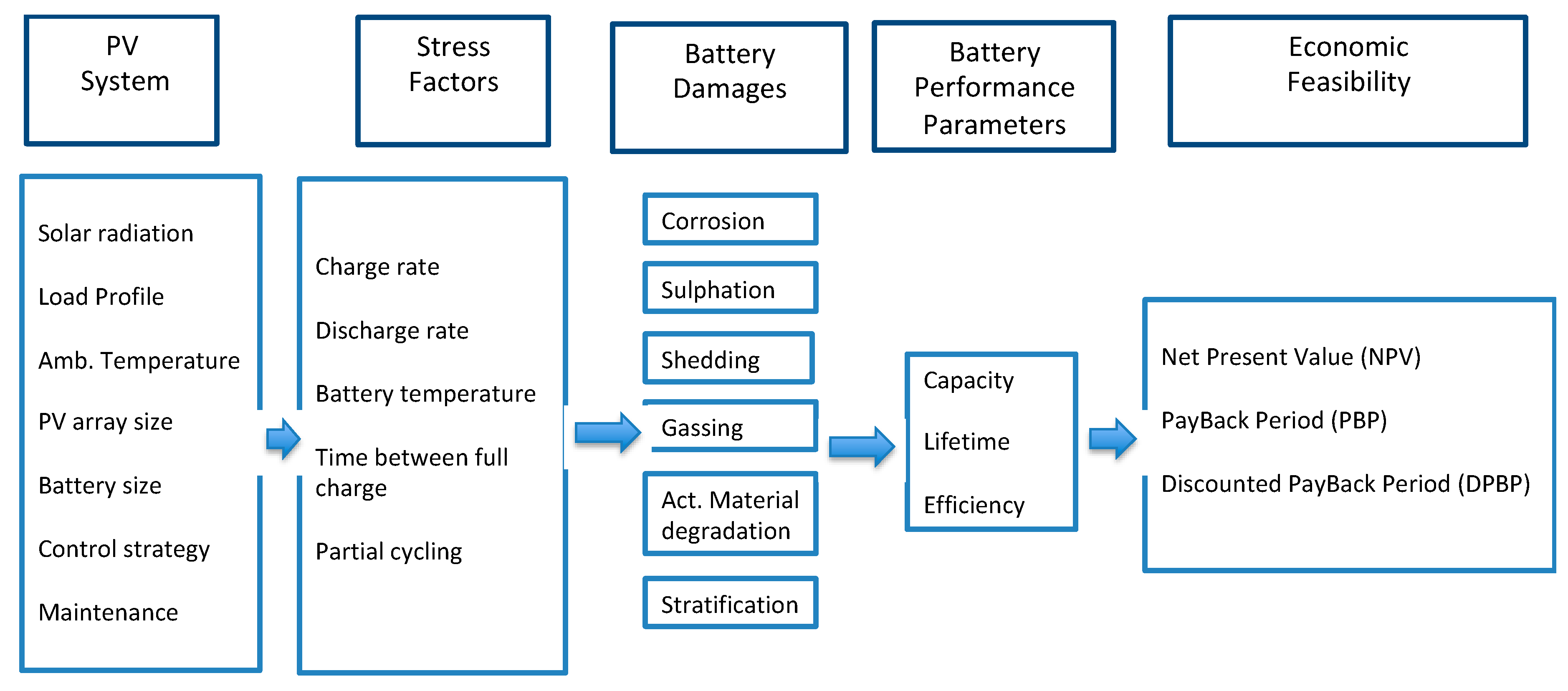
According to Figure 1, the relationship between the photovoltaic system, stress factors, battery damages, and battery performance parameters is described for each stress factor in the following paragraphs.

Discharge Rate

Discharge rate is the rate of discharge as compared to the capacity of the battery under standard operating conditions. The capacity of a battery is commonly rated at 1 C, meaning that a fully charged battery rated at 200 Ah should provide 200 A for 1 h. The same battery discharging at 0.5 C should provide 100 A for 2 h, and at 2 C it delivers 400 A for 30 min.

Discharge rate stress factor damages the battery as follows. When the battery is discharged, sulphate crystals are created at both electrodes. If sulphate crystals are not dissolved, they could damage the electrodes by corrosion or mechanical effect, reducing their lifetime. The battery capacity decreases with the active material degradation leading to an increase in the internal resistance, which negatively affects the battery efficiency. In addition, at a high discharge rate, the battery voltage drops. Low voltage also induces control corrosion damage, which may be avoided with voltage control. It is therefore advisable to avoid deep discharges if the load profile allows it. However, there is a positive effect at a high discharge rate. This is the decrease of the electrolyte stratification.

Energy load profile is one of the main parameters that affect the discharge rate because a higher load profile leads to a higher discharge rate. Nevertheless, this higher discharge rate should be lower if the photovoltaic array yield is high in that instant, decreasing the energy required from the battery. So, the PV array size and solar radiation profile also have a significant influence on this stress factor. In addition, a high or low discharge rate is always referred to battery capacity, so battery size also affects this stress factor. Lastly, but no less important, is the control strategy. When and how the battery discharge is allowed has a significant influence on the discharge rate. Control strategy could limit the maximum discharge rate allowed. So, the influence of the PV system on this stress factor could be reduced if the control strategy limits high discharge rates and there is an appropriate sizing of the battery and PV array according to solar radiation and load demand profiles.

Charge Rate

Charge rate is the rate of charge as compared to the capacity of the battery under standard operating conditions. Charge rate stress factor damages the battery as follows. When the battery is charged with a high charge rate, it leads to active mass shedding, water loss due to gassing that reduces the coulombic efficiency and corrosion processes.

Photovoltaic array yield is the main parameter that affects the charge rate. So, the photovoltaic array size and the solar radiation profiles have a significant influence on this stress factor. A high or low charge rate is always referred to battery capacity, so battery size affects this stress factor similarly to discharge rate stress factor. Control strategy plays a significant role in limiting the charge rate. As happens with the discharge rate stress factor, the influence of the photovoltaic system on this stress factor could be reduced if the control strategy limits high charge rates and there is an appropriate sizing of the battery and PV array according to solar radiation and load demand profiles.

Time between Full Charge

Time between full charge is the time in days between recharging the battery up to SoC > 90%. The time between the full state of charge is an average value for one year of operation. If the time between full state of charge is too long, lead sulphate crystals will grow and form hard sulphation which is impossible to convert back to charged material under normal operating conditions. Long time between full charge at a low SoC could lead to stratification and corrosion processes if the battery temperature is high.

Photovoltaic array yield and load profiles are the main parameters that affect this time. In addition, the control strategy about the allowed time between full charge has a significant influence on the damages. Control strategy could limit the damages and the impact of the photovoltaic system on this stress factor.

Battery Temperature

Battery temperature is one of the main stress factors of a battery that significantly affects it when the battery temperature is out of the range 10–25 °C. Battery temperature is affected by the room temperature that, in turn, is usually related to the ambient temperature. In addition, charge and discharge rate also affect the battery temperature [33]. Battery temperature affects all of the main performance parameters of the battery such as capacity, lifetime, and efficiency.

High temperature leads mainly to corrosion. In addition, other damages such as sulphation, water loss, and active material degradation could appear. Water losses increase with increasing battery temperature according to the Arrhenius law. Gassing reduces the coulombic efficiency and results in the mixing of the electrolyte in flooded batteries. Low temperature reduces the capacity and increases internal resistance. Extreme temperatures could lead to freezing of the electrolyte especially when the battery is at a low SoC when electrolyte density is minimum. If the temperature is properly controlled around moderate values, its impact on damage should be medium.

To control this stress factor from the photovoltaic system, an adequate selection of the battery room is necessary including a refrigeration strategy in case of need. In addition, recommendations to avoid a high charge and discharge rate should be taken into account as described above. When lead–acid batteries are used in applications with shallow cycling, their service life normally is limited by float life. In systems where the cycling is deep, but occurs only a few times a year, the temperature-dependent corrosion process is the normal life-limiting factor, even for batteries with short cycle life. In systems with deep daily cycling, the cycle life determines the service life of the battery. As the temperature increases, the electrochemical activity of the battery increases as well as the rate of the natural ageing of the active material. Elevated temperatures result in accelerated ageing but also higher available capacity [34]. Manufacturer datasheets show battery parameters for a range of temperature between 20–25 °C and most manufacturers give the effect of temperature on the capacity, efficiency, and lifetime. [14].

Ah-Throughput

This factor is expressed as cumulative Ah discharged per year and it is normalised in units of the battery nominal capacity. A high Ah-throughput increases active mass degradation, active mass shedding, and electrolyte stratification. The full impact of the Ah-throughput on ageing processes can only be discussed when other stress factors such as cycling at partial state of charge and time at a low state of charge are considered at the same time. Most of the investigated systems show an annual Ah-throughput of 10–100 times the rated capacity [35].

Partial Cycling

The partial cycling factor represents a cumulative Ah-throughput in (%) in specified SoC ranges. Partial cycling occurs when the charge and discharge processes are not complete. Battery damage mainly depends on the frequency, state of charge and temperature. This is a significant stress factor in photovoltaic systems because it is very difficult to avoid. The charge process is mainly stochastic due to the solar radiation and, to the fact that the discharge process depends on the load demand profile that in many cases also is stochastic.

High frequency of partial cycling leads to high voltage variations that could cause corrosion with an increase in the internal resistance and, thus a decrease in capacity and efficiency. In addition, according to the state of charge, partial cycling could lead to damages such as sulphation and stratification, and active material degradation could appear. During battery operation, the electrodes suffer from strong mechanical stress due to the large variations in the volume of the active materials involved in the charge and discharge processes. This causes the separation of the active material from the electrodes leading to a decrease in porosity and surface area of the electrolyte and active material boundary, reducing the effective capacity, efficiency, and lifetime of the battery. This degradation is a result of its exact discharge and charge history and cannot be restored. [36]. This effect is stressed by an increase in DoD during the daily cycles of PV systems [9].

Time at a Low SoC

The time at a low SoC in the n-year is defined as the cumulative operating hours in percent of the whole hour of a year at an SoC below a minimum value. For instance, SoC < 35%.

The main impact when the battery is at a low state of charge is irreversible sulphation that leads to a decrease in battery capacity and lifetime. In addition, voltage battery and acid density are low and could lead to corrosion, increasing the internal resistance and decreasing the capacity and efficiency. This stress factor is particularly relevant for lead–acid batteries. Time at a low SoC mainly occurs when the power from the photovoltaic array is much lower than the load demand. That is to say, photovoltaic energy self-consumption energy is low compared to the load demand. When the battery temperature is very low, barely below 0 °C, its electrolyte stratification should be low, and the state of charge should be as high as possible to avoid electrolyte freezing.

To avoid this effect, it should be required a proper control strategy to avoid energy consumption if the SoC of the battery is low for a long time. So, in some cases, load demand could not be satisfied by the PV system and, in some cases, the battery could be charged from the grid.

The battery damages are a result not only of the influence of each stress factor, but of the combination among all the “stress factors”. Thus, special care shall be taken to select the battery, the control of the DoD, charge and discharge rates, room temperature, electrolyte stratification, time between full charge, and time at a low SoC.

2.2. Battery Performance Parameters

Battery Lifetime

Battery lifetime is generally expressed as the loss of the battery’s ability to provide a specific amount of its original nominal capacity, usually 80%. One of the main drawbacks of lead–acid batteries is its short lifetime, about 1000 cycles at 80% DoD [28]. The addition of activated carbon into the negative plate of the lead–acid battery can greatly enhance its lifetime [34]. The reasons for this short battery lifetime are due to the ageing mechanism described, mean grid corrosion on the positive electrode, depletion of the active material, and expansion of the positive plates. Such ageing phenomena are accelerated at high battery temperature and high discharge rate. Battery lifetime is often directly linked to the thickness of the positive plates. The thicker the plates, the longer the life will be. During charging and discharging, the lead on the plates gets gradually washed away and the sediment falls to the bottom. The weight of a battery is a good indicator of the lead content and life expectancy.

Predicting the lifetime of lead–acid batteries in PV systems with irregular operating conditions such as partial state of charge cycling, varying depths of discharge, and different times between full charging is known as a difficult task [30].

High battery temperature and DoD accelerate the ageing phenomena, grid corrosion on the positive electrode, depletion of active material, and expansion of the positive plates and sulphation processes. Many researchers assume that battery temperature is ambient temperature.

Battery temperature shall nevertheless be affected by the rate of charge/discharge as well as by ambient temperature [26]. The Arrhenius Law describes the battery temperature influence on the chemical reaction. As a rule, for lead–acid batteries each 10 °C increase in temperature reduces service life by 50% [25,31]. Other researchers predict the battery lifetime taking into account the battery temperature and the annual cycles. For instance, Rydh et al. [32], use Equation (1).

$${\mathrm{t}}_{\mathrm{DoD},\mathrm{T}}=\frac{{\mathrm{N}}_{\mathrm{DoD},25°\mathrm{C}}}{{\mathrm{n}}_{\mathrm{DoD},\mathrm{T}}}·{\mathsf{\sigma }}_{\left(\mathrm{T}\right)}$$

(1)

where ${\mathrm{t}}_{\mathrm{DoD},\mathrm{T}}$ is the battery lifetime in years, at a given DoD and temperature T, ${\mathrm{N}}_{\mathrm{DoD},25°\mathrm{C}}$ is the battery cycles from the manufacturer datasheet at a given DoD and 25 °C, ${\mathrm{n}}_{\mathrm{DoD},\mathrm{T}}$ is the annual cycles at a given DoD and temperature T, according to the operating conditions, and ${\mathsf{\sigma }}_{\left(\mathrm{T}\right)}$ is a lifetime correction factor dependent on the temperature. For a lead–acid battery at a temperature T, the ${\mathsf{\sigma }}_{\left(\mathrm{T}\right)}$ value is shown in

Table 1. Lead–acid battery lifetime correction factor dependent on the temperature.

${\mathsf{\sigma }}_{25°\mathbf{C}}$	${\mathsf{\sigma }}_{30°\mathbf{C}}$	${\mathsf{\sigma }}_{35°\mathbf{C}}$	${\mathsf{\sigma }}_{40°\mathbf{C}}$	${\mathsf{\sigma }}_{45°\mathbf{C}}$	${\mathsf{\sigma }}_{50°\mathbf{C}}$
1	0.69	0.51	0.37	0.25	0.14

.

Battery DoD influence on the battery lifetime appears to be logarithm and it is given by the manufacturer [26]. Thus, if the battery temperature is constant, the number of cycles yielded by a battery goes up exponentially the shallower the DoD.

Taking into account other stress factors, according to the scenario conditions, Equation (1) has been modified by coefficient $\mathsf{\alpha }$ that depends on the scenario given in Equation (2):

$${\mathrm{t}}_{\mathrm{DoD},\mathrm{T}}=\mathsf{\alpha }·\frac{{\mathrm{N}}_{\mathrm{DoD},25°\mathrm{C}}}{{\mathrm{n}}_{\mathrm{DoD},\mathrm{T}}}·{\mathsf{\sigma }}_{\left(\mathrm{T}\right)}$$

(2)

where $\mathsf{\alpha }$ is a degradation factor related to the operating conditions.

Battery Efficiency

Battery efficiency is mainly affected by the active material, temperature, state of charge, charge, and discharge rate. Under the right temperature, SoC, new and with moderate charge and discharge rate, lead–acid provides high charge and discharge efficiency, between 80% and 90% [34].

The Homer software assumes that the charge efficiency and the discharge efficiency are both equal to the square root of the round-trip efficiency. The battery round-trip efficiency is the round-trip DC-to-storage-to-DC energy efficiency of the storage bank, or the fraction of energy put into the storage that can be retrieved, and typically, it is about 80%, without degradation over its lifetime.

There are several simplified models to estimate battery efficiency. The Jenkins model [37] gives a simplified model based on empirical data, according to battery capacity and charge and discharge rate. The main drawbacks of this model are that it does not take into account the SoC of the battery. The CIEMAT model [38] takes into account the SoC and the charge rate showing a good performance to represent dynamic and more complex battery operating conditions [39] according to Equation (3).

$${\mathsf{\eta }}_{\mathrm{bc},\mathrm{t},1}=1-\exp \left[\frac{20.73}{\frac{{\mathrm{I}}_{\mathrm{c},\mathrm{t}}}{{\mathrm{I}}_{10}}+0.55}·\left(\mathrm{SoC}-1\right)\right]$$

(3)

where ${\mathsf{\eta }}_{\mathrm{bc},\mathrm{t},1}$ is the charge efficiency of the battery at the hour t the first year without degradation damages and ${\mathrm{I}}_{\mathrm{c},\mathrm{t}}$ represents the charge current in that hour. This equation shows that charge efficiency at very low charge current, medium SoC, 25 °C, and the battery new, could be near 99%. If the charge current is high (five times I₁₀) and SoC is high (90%), charge efficiency is reduced to near 30%. Discharge efficiency has a similar equation. The CIEMAT model does not include the degradation process caused by the other stress factors that lead to active material degradation, sulphation, stratification, and corrosion processes. Taking into account these degradation processes, Equation (3) has been modified including coefficient $\mathsf{\gamma }$ that depends on the operating conditions given in Equation (4):

$${\mathsf{\eta }}_{\mathrm{bc},\mathrm{t},\mathrm{n}}={\left(1-\mathsf{\gamma }\right)}^{\mathrm{n}}·\left[1-\exp \left[\frac{20.73}{\frac{{\mathrm{I}}_{\mathrm{c},\mathrm{t}}}{{\mathrm{I}}_{10}}+0.55}·\left(\mathrm{SoC}-1\right)\right]\right]$$

(4)

Capacity

Most battery manufacturers specify the capacity of their batteries for a certain discharge time of hour t (h) and the temperature range is 20–25 °C. For example, C_t (25 °C) = 500 Ah. This means that the battery will deliver 500 Ah if discharged at such a rate that the discharge time is t hours at 25 °C. Using this example, if t = 10 h, the rate would be I₁₀= 50 A. Kim et al. [40] highlight that batteries in real-use conditions lose their capacity considerably quicker than suggested by manufacturers.

The Peukert equation can be used in a simple way for calculating the available capacity C_t2 at a different discharge rate I_t2 and a constant temperature of 25 °C using Equation (5):

$${\mathrm{C}}_{\mathrm{t}2}\left(25°\mathrm{C}\right)={\mathrm{C}}_{\mathrm{t}1}\left(25°\mathrm{C}\right)·{\left(\frac{{\mathrm{I}}_{\mathrm{t}2}}{{\mathrm{I}}_{\mathrm{t}1}}\right)}^{\mathrm{PC}-1}$$

(5)

where PC is the Peukert coefficient. Nevertheless, the Peukert equation does not take into account temperature fluctuation, variable current of discharge, and ageing, and it is not accurate for low discharge rates due to the influence of the self-discharge rate [41,42].

The relationship between battery capacity and temperature is given in the standard EN 60896-11 [43] according to Equation (6):

$${\mathrm{C}}_{\mathrm{t}}\left({\mathrm{T}}_1\right)={\mathrm{C}}_{\mathrm{t}}\left(25°\mathrm{C}\right)·\left(1+\mathsf{\lambda }·\left({\mathrm{T}}_1-25°\mathrm{C}\right)\right)$$

(6)

where λ is 0.006 when the battery discharge time is lower or equal than 3 h and 0.01 when the battery discharge time is higher than 3 h.

The CIEMAT model [38] gives the lead–acid battery capacity C normalised with respect to discharge current corresponding to C₁₀ rated capacity I₁₀, corrected by temperature, given by Equation (7):

$$\frac{\mathrm{C}}{{\mathrm{C}}_{10}}=\frac{1.67}{1+1.67·{\left(\mathrm{I}/{\mathrm{I}}_{10}\right)}^{0,9}}·\left(1+0.005·\left(\mathrm{T}-25°\mathrm{C}\right)\right)$$

(7)

when the discharge current tends to 0, the maximum capacity that can be removed is about 67% over C₁₀ capacity at 25 °C.

Witold et al. [44] analyse ageing mechanisms on battery capacity, concluding with the function C(x, y) = (ax² + bx + c)·(dy² + ey + f), where x is the number of cycles and y is the DoD, according to the battery and PV system sizes.

In conclusion, the effective capacity of the battery in a PV system depends mainly on the discharge rate, DoD, temperature, and ageing effects. These stress factors are affected by the battery size, load profile, solar radiation profile, battery room temperature, and control strategy.

According to Witold results, a battery capacity degradation parameter $\delta$ is proposed according to Equation (8):

$${\mathrm{C}}_{\mathrm{t},\mathrm{n}}={\left(1-\mathsf{\delta }\right)}^{\mathrm{n}}·{\mathrm{C}}_{\begin{array}{c}t,1\end{array}}$$

(8)

2.3. Battery Operation Scenarios According to PV System Operating Conditions

As shown, PV array and battery sizes, solar radiation, ambient temperature, load demand, and control strategy have a significant influence on those stress factors, degradation processes, and battery damages. Consequently, battery performance parameters are affected by these damages. The main battery performance parameters are lifetime, charge and discharge efficiency, and capacity.

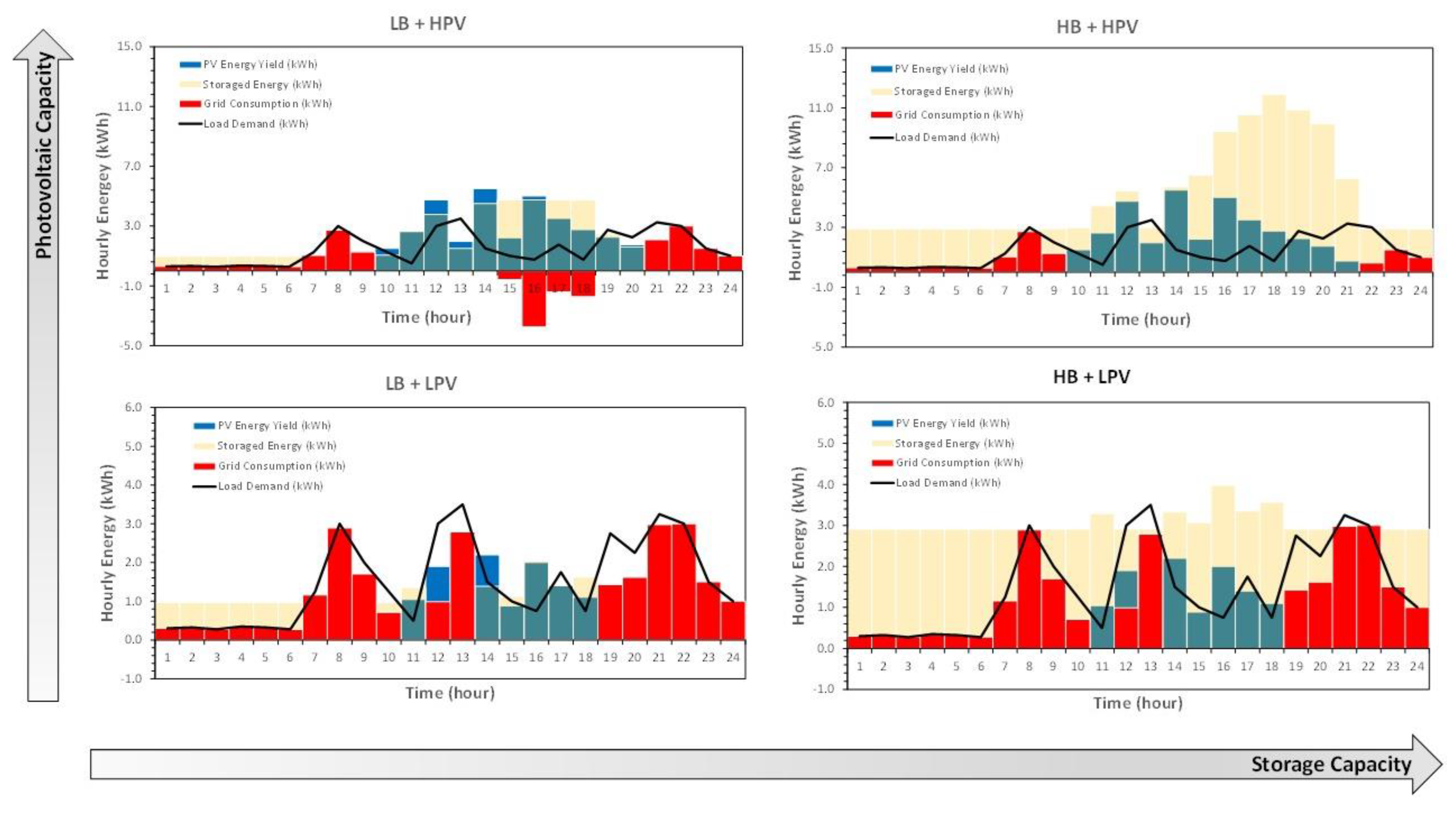
All of the main battery operation combinations can be classified under four scenarios:

(1)

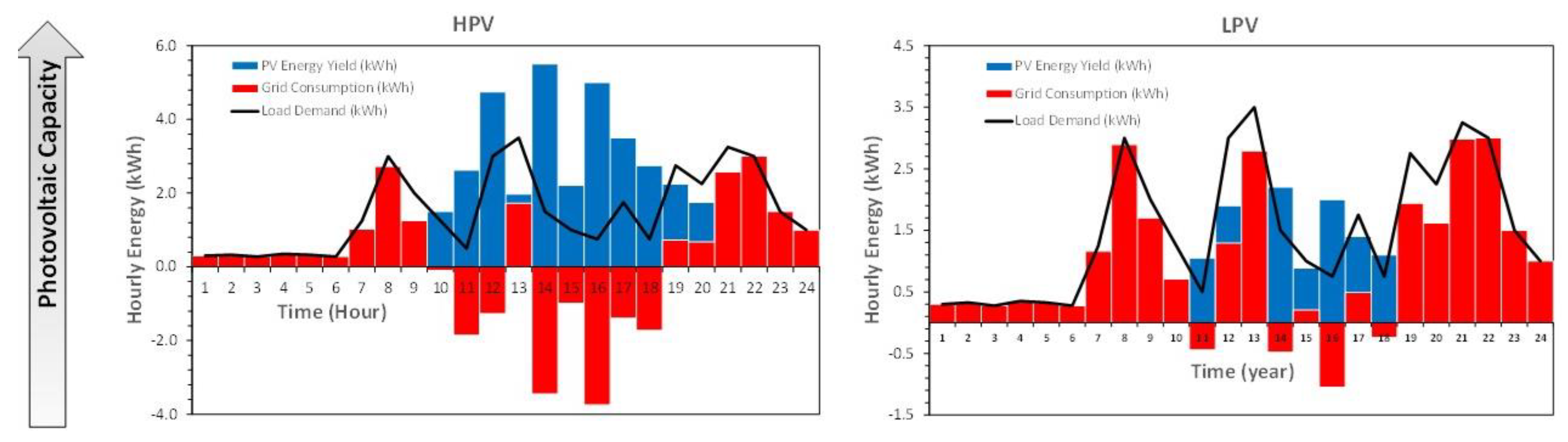
Low Battery and High PV yield (LB + HPV): This happens when the battery capacity is small with respect to the PV array yield and the PV array yield is in the same order of magnitude or higher than the load demand.

In this scenario, battery operating conditions are characterised by a very high to medium Ah-throughput, deep partial cycling, low time between full charge, full recharge, and low time at a high SoC, with high to very high discharge and charge rates. The temperature is according to room conditions and very affected by charge and discharge rate [27].

The consequences of these operating conditions are that the battery suffers from high to very high sulphation, high active material degradation, and high electrolyte stratification, high water loss, and medium-high corrosion processes according to battery temperature. This could be the worst condition for a lead–acid battery.

(2)

Low Battery and Low PV yield (LB + LPV): This happens when the battery capacity is small with respect to the PV array yield and the PV array yield is smaller than the load demand.

The operation of the battery is characterised by a low Ah-throughput, frequent partial cycling, deep discharges with high discharge, and low-medium charge rates. These may occur for a long time at a low SoC and medium-high time between full charge. Battery temperature will match room conditions and be mildly affected by the charge rate.

The consequences of these operating conditions are that the battery suffers from high to very high sulphation, high active material degradation and low electrolyte stratification, low water loss, and low–medium–high corrosion processes according to battery temperature. This could be the second worse condition for a lead–acid battery.

(3)

High Battery and High PV yield (HB + HPV): This happens when the battery capacity is high with respect to the PV array yield and the PV array yield is in the same order of magnitude or higher than the load demand.

In this scenario, battery operating conditions are characterised by a very low Ah-throughput with very shallow partial cycling, low time between full charge, full recharge is usual and low time at a high SoC, and low discharge and charge rates. The temperature is according to room conditions and slightly affected by high discharge and charge rates. Those could be the second optimal conditions for a lead–acid battery.

The consequences of these operating conditions are that the battery suffers from low-medium corrosion processes if the battery temperature is high with low water loss, low-medium sulphation, low active material degradation, and medium-high electrolyte stratification processes.

(4)

High Battery and Low PV yield (HB + LPV): This happens when the battery capacity is high with respect to the PV array yield and the PV array yield is smaller than the load demand.

In this scenario, battery operating conditions are characterised by a very low Ah-throughput with partial cycling and high DoD, with a low discharge rate and a low-medium charge rate, long time at a low SoC, and high time between full charge. The temperature is according to room conditions and not affected by high charge rates. Those could be the better conditions for a lead–acid battery.

The consequences of these operating conditions are that the battery suffers from medium corrosion, low water loss, low-medium sulphation, low active material degradation, and high electrolyte stratification processes.

In addition, real negative consequences for the four scenarios also depends very much on the lead–acid battery technology such as a flooded lead–acid battery, Absorbed Glass Mat Batteries (AGM), valve-regulated lead–acid (VRLA), sealed lead–acid (SLA)), and the control strategy including the battery charge/discharge controller. There is mature technology available on the market with intelligent and flexible battery management systems that allow adequate commissioning and setting of the main parameters of the battery, reducing the effects of the stress factors on battery degradation. If the battery parametrisation is not very well done, it can be worse for battery degradation than any other factor.

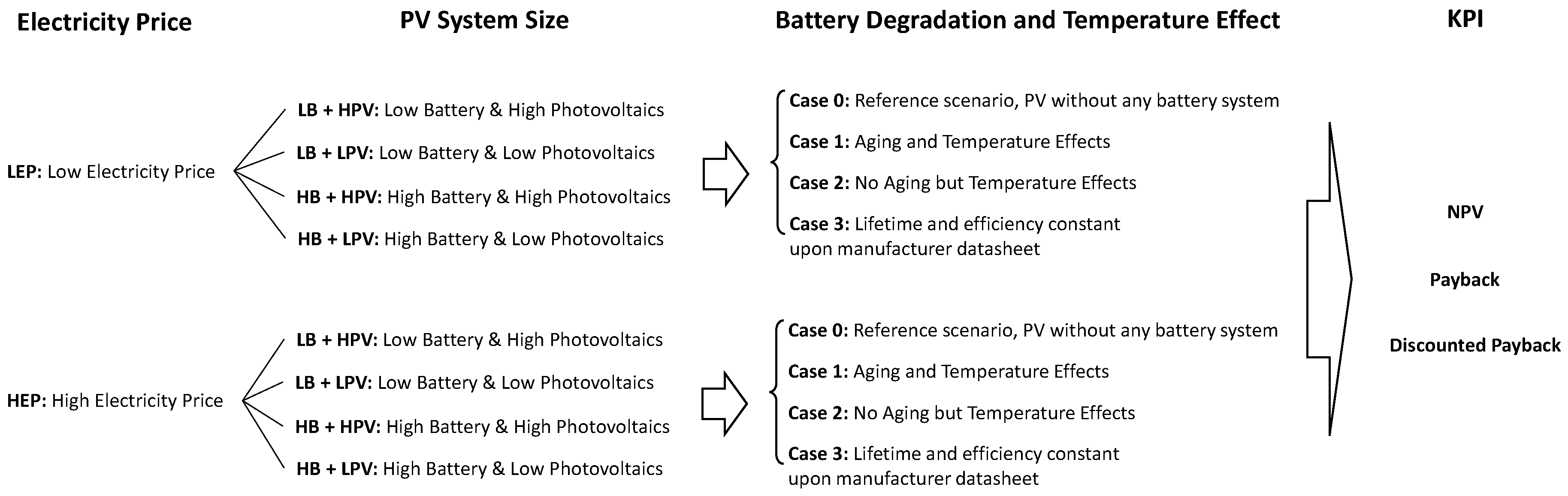
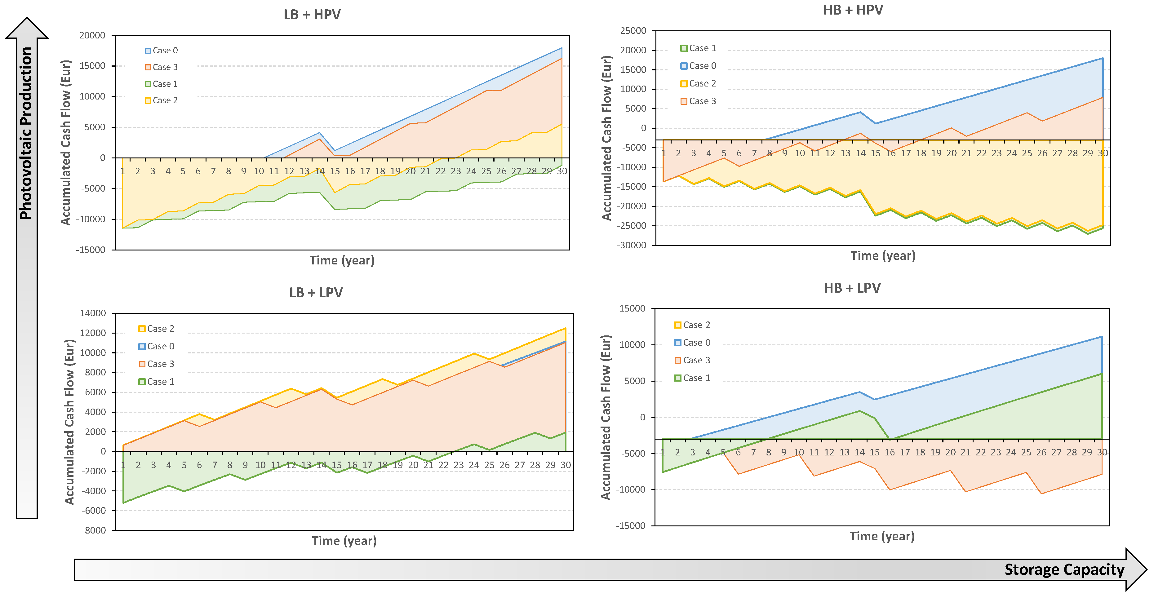
As a result, four alternatives have been taken into account to analyse the influence of the degradation process in lead–acid battery on technoeconomic studies:

• Case 0—Technoeconomic analysis assumes that the PV system does not have a battery. This will be the reference case.
• Case 1—Technoeconomic analysis assumes that battery lifetime and battery efficiency depend on degradation factors, σ(T), α, γ_d, and γ_c.
• Case 2—Technoeconomic analysis assumes that battery lifetime and battery efficiency depend on degradation factors σ(T) but not on α, γ_d, and γ_c.
• Case 3—Technoeconomic analysis assumes that battery lifetime and battery efficiency are constants according to the manufacturer datasheet. So, they do not depend on the degradation factors σ(T), α, γ_d, and γ_c.

The α, ${\mathsf{\gamma }}_{\mathrm{d}}$, and ${\mathsf{\gamma }}_{\mathrm{c}}$ values should be validated according to the lead–acid battery technology. This technoeconomic study does not include the capacity degradation processes that will be included in further studies.

3. Energy Balance

According to Figure 2, the electricity produced by the PV array can be directly consumed by the household totally or partially. If the household hourly electricity load ${\mathrm{E}}_{\mathrm{load},\mathrm{t},\mathrm{n}}$ is higher than the PV array hourly electricity ${\mathrm{E}}_{\mathrm{PVa},\mathrm{t},\mathrm{n}},$ all the PV array yield will be self-consumed and the battery could provide electricity to the load. If there is enough capacity in the battery, part or all of the excess electricity will be stored in the battery within its limits. If the battery is already fully charged, the remaining PV array electricity is then sold to the grid, ${\mathrm{SE}}_{\mathrm{GRID},\mathrm{t},\mathrm{n}}.$

According to Figure 2, when the hourly electricity load ${\mathrm{E}}_{\mathrm{load},\mathrm{t},\mathrm{n}}$ is lower than the PV array hourly electricity, all the PV array electricity is self-consumed. If there is enough energy in the battery, ${\mathrm{E}}_{\mathrm{BAT},\mathrm{t},\mathrm{n}}$ all or part of the remaining electricity load will be met by the battery, ${\mathrm{E}}_{\mathrm{BAT},\mathrm{t},\mathrm{n}}^{-}.$ If the battery is empty, and the electricity load has not been satisfied by PV array and battery the remaining electricity load will be provided by the grid. ${\mathrm{BE}}_{\mathrm{GRID},\mathrm{t},\mathrm{n}}.$ All the battery charge and discharge processes will be affected by the charge and discharge efficiency. PV array yield and battery discharge are also affected by the inverter efficiency when electricity is self-consumed or sold to the grid.

The following assumptions have been done to focus on the degradation effects on lead–acid batteries in technoeconomic studies:

-

The annual hourly solar irradiance on the PV array and load demand profiles are the same during all days and years. PV system lifetime is set at 30 years. PV module degradation over the years has been despised.

-

A typical day has been selected with a solar radiation, ambient temperature, and load demand profile.

-

The Inverter efficiency is constant over its lifetime and set at 90%. The inverter lifetime is set at 15 years.

-

The Performance Ratio (PR) is constant over the PV system lifetime and is set at 90% [45].

-

The battery self-discharge rate is depreciable. The upper and lower state of charge (SoC) of the battery should be defined. The suggested values (used for this study) are 100% and 20%, respectively.

-

The Electricity retail price and electricity surplus price are constants over the PV system lifetime.

The energy output of a PV array for an hour t of the year n, in kWh, ${\mathrm{E}}_{\mathrm{PVa},\mathrm{t},\mathrm{n}}$ is given by Equation (9):

$${\mathrm{E}}_{\mathrm{PVa},\mathrm{t},\mathrm{n}}={\mathrm{P}}_{\mathrm{PV}}·\left({\mathrm{H}}_{\mathrm{g},\mathrm{t},\mathrm{n}}/1000\right)·\left(1-\mathsf{\beta }·\left({\mathrm{T}}_{\mathrm{P},\mathrm{t},\mathrm{n}}-25\right)\right)$$

(9)

where ${\mathrm{P}}_{\mathrm{PV}}$ is the peak power of the PV array, in kWp, ${\mathrm{H}}_{\mathrm{g},\mathrm{t},\mathrm{n}}$ is the global solar radiation on the PV array expressed in Wh/m² for an hour t of the year n, $\mathsf{\beta }$ is PV module power temperature coefficient given by the manufacturer in %/(100 °C), and ${\mathrm{T}}_{\mathrm{P},\mathrm{t},\mathrm{n}}$ is the average module temperature in °C, for an hour t of the year n.

After a review of several models, the nominal operating cell temperature model was chosen to estimate the average module temperature for an hour t, owing to its simplicity, adequacy of its predicted temperatures for PV applications, and the wider availability of input data. According to the photovoltaic module building intergradation, other models could be used [46]. Therefore, ${\mathrm{T}}_{\mathrm{p},\mathrm{t},\mathrm{n}}$ is given according to Equation (10):

$${\mathrm{T}}_{\mathrm{p},\mathrm{t},\mathrm{n}}={\mathrm{T}}_{\mathrm{a},\mathrm{t},\mathrm{n}}+\frac{\left(\mathrm{NOCT}-20\right)}{800}·{\mathrm{H}}_{\mathrm{g},\mathrm{t},\mathrm{n}}$$

(10)

where ${\mathrm{T}}_{\mathrm{a},\mathrm{t},\mathrm{n}}$ is the average ambient temperature in °C for an hour t of the year n, NOCT is the Nominal Operating Cell Temperature (NOCT) in °C given by the PV module manufacturer.

The output energy of a PV system without battery for an hour t can be calculated as the energy output of a PV array affected by the balance of system (BoS) losses such as inverter, cables, dirt in the PV modules, PV module mismatching. These losses have been included in the Performance Ratio (PR). PV system yield, without battery, for an hour t of the year n, in kWh, ${\mathrm{E}}_{\mathrm{PV},\mathrm{t},\mathrm{n}}$ is calculated according to Equation (11):

$${\mathrm{E}}_{\mathrm{PV},\mathrm{t},\mathrm{n}}={\mathrm{E}}_{\mathrm{PVa},\mathrm{t},\mathrm{n}}·\mathrm{PR}$$

(11)

There are two interesting ratios, the photovoltaic self-consumption ratio, ${\mathrm{SCR}}_{\mathrm{t}}$ defined as the ratio between the self-consumption energy from the PV system, and the total photovoltaic energy yield for an hour t, is given by Equation (12):

$${\mathrm{SCR}}_{\mathrm{t},\mathrm{n}}=\frac{{\mathrm{E}}_{\mathrm{PV},{\mathrm{S}}_{\mathrm{C}},\mathrm{t},\mathrm{n}}}{{\mathrm{E}}_{\mathrm{PV},\mathrm{t},\mathrm{n}}}$$

(12)

where the load self-consumption ratio, ${\mathrm{LSCR}}_{\mathrm{t},\mathrm{n}}$, defined as the ratio between the self-consumption energy from the PV system and the load demand ${\mathrm{E}}_{\mathrm{Load},\mathrm{t},\mathrm{n}}$, for an hour t, can be calculated by Equation (13):

$${\mathrm{LSCR}}_{\mathrm{t},\mathrm{n}}=\frac{{\mathrm{E}}_{\mathrm{PV},{\mathrm{S}}_{\mathrm{C}},\mathrm{t},\mathrm{n}}}{{\mathrm{E}}_{\mathrm{Load},\mathrm{t},\mathrm{n}}}$$

(13)

There are several situations according to the hourly energy balance between the load demand, PV system yield, and state of the battery for every hour t. They are grouped into two global situations, A and B. According to the energy balance between the PV system yield and load demand, each is disaggregated on the basis of the state of the battery in two more scenarios and another situation, Situations C, which occurs when there is no battery.

(a)

Situation A: PV system with battery. The PV system yield is higher or equal to the load demand, ${\mathrm{E}}_{\mathrm{PV},\mathrm{t},\mathrm{n}}\ge {\mathrm{E}}_{\mathrm{load},\mathrm{t},\mathrm{n}}.$ When the PV system yield is higher than load demand, ${\mathrm{E}}_{\mathrm{load},\mathrm{t},\mathrm{n}},$ the entire load demand is met by the PV system. In this case, the energy self-consumed by household, ${\mathrm{E}}_{\mathrm{PV},{\mathrm{S}}_{\mathrm{C}},\mathrm{t},\mathrm{n}}={\mathrm{E}}_{\mathrm{Load},\mathrm{t},\mathrm{n}},$ the bought energy from the national grid, ${\mathrm{BE}}_{\mathrm{GRID},\mathrm{t},\mathrm{n}}=0,$ the discharged energy from the battery for an hour t of the year n, ${\mathrm{E}}_{\mathrm{BAT},\mathrm{t},\mathrm{n}}^{-}=0$, and ${\mathrm{LSCR}}_{\mathrm{t},\mathrm{n}}=1.$

In addition, according to the battery state can occur in three more situations.

Situation A.1—This situation occurs when the battery has enough capacity to store the excess energy for an hour t. That is, Equation (14) should be fulfilled:

$${\mathrm{E}}_{\mathrm{BATfull},\mathrm{t}}-{\mathrm{E}}_{\mathrm{BAT},\mathrm{t}-1,\mathrm{n}}\ge {\mathrm{E}}_{\mathrm{BAT},\mathrm{t},\mathrm{n}}^{+}$$

(14)

where ${\mathrm{E}}_{\mathrm{BATfull},\mathrm{t}}$ is the maximum energy that the battery could store, ${\mathrm{E}}_{\mathrm{BAT},\mathrm{t}-1,\mathrm{n}}$ is the energy stored in the battery at the end of the hour (t−1) of the year n, and ${\mathrm{E}}_{\mathrm{BAT},\mathrm{t},\mathrm{n}}^{+}$ is the charged energy into the battery for an hour t of the year n. This is given by Equation (15):

$${\mathrm{E}}_{\mathrm{BAT},\mathrm{t},\mathrm{n}}^{+}=\left({\mathrm{E}}_{\mathrm{PVa},\mathrm{t},\mathrm{n}}-\left({\mathrm{E}}_{\mathrm{load},\mathrm{t},\mathrm{n}}/\mathrm{PR}\right)\right)·{\mathsf{\eta }}_{\mathrm{bc},\mathrm{t},\mathrm{n}}$$

(15)

where ${\mathsf{\eta }}_{\mathrm{bc},\mathrm{t},1}$ is the battery charge efficiency for an hour t in the first year, given by Equation (16):

$${\mathsf{\eta }}_{\mathrm{bc},\mathrm{t},1}=0.9-\exp \left[\frac{20.73}{\frac{\left(\left({\mathrm{E}}_{\mathrm{PVa},\mathrm{t},1}-\left({\mathrm{E}}_{\mathrm{Load},\mathrm{t}},1/\mathrm{PR}\right)\right)/{\mathrm{V}}_{\mathrm{nb}}\right)}{{\mathrm{I}}_{10}}+0.55}·\left(\frac{{\mathrm{E}}_{\mathrm{BAT},\mathrm{t}-1,1}}{{\mathrm{E}}_{\mathrm{BATfull}}}-1\right)\right]$$

(16)

where V_nb is the battery nominal voltage according to the battery cells connected in series. For the following years n, it could be assumed a battery charge efficiency degradation factor ${\mathsf{\gamma }}_{\mathrm{c}},$ used in Equation (17) and with the values shown in

Table 2. Battery charge efficiency degradation factor: ${\mathsf{\gamma }}_{\mathrm{c}}.$

Scenario	LB + HPV	LB + LPV	HB + HPV	HB + LPV
${\mathsf{\gamma }}_{\mathrm{c}}$	0.3	0.2	0.1	0.05

.

$${\mathsf{\eta }}_{\mathrm{bc},\mathrm{t},\mathrm{n}}={\left(1-{\mathsf{\gamma }}_{\mathrm{c}}\right)}^{\mathrm{n}}·{\mathsf{\eta }}_{\mathrm{bc},\mathrm{t},1}$$

(17)

The stored energy in the battery and the end of the hour t is given by Equation (18):

$${\mathrm{E}}_{\mathrm{BAT},\mathrm{t},\mathrm{n}}={\mathrm{E}}_{\mathrm{BAT},\mathrm{t}-1,\mathrm{n}}+{\mathrm{E}}_{\mathrm{BAT},\mathrm{t},\mathrm{n}}^{+}$$

(18)

In this scenario, ${\mathrm{SE}}_{\mathrm{GRID},\mathrm{tn}}=0$.

Situation A.2—This situation occurs when the battery does not have enough storage capacity to storage all the excess energy. That is, Equation (19) should be fulfilled:

$${\mathrm{E}}_{\mathrm{BATfull}}-{\mathrm{E}}_{\mathrm{BAT},\mathrm{t}-1,\mathrm{n}}<\left({\mathrm{E}}_{\mathrm{PVa},\mathrm{t},\mathrm{n}}-\left({\mathrm{E}}_{\mathrm{load},\mathrm{t},\mathrm{n}}/\mathrm{PR}\right)\right)·{\mathsf{\eta }}_{\mathrm{bc},\mathrm{t},\mathrm{n}}$$

(19)

${\mathrm{E}}_{\mathrm{BAT},\mathrm{t},\mathrm{n}}^{+}$ is given now by Equation (20):

$${\mathrm{E}}_{\mathrm{BAT},\mathrm{t},\mathrm{n}}^{+}=\left({\mathrm{E}}_{\mathrm{BATfull}}-{\mathrm{E}}_{\mathrm{BAT},\mathrm{t}-1,\mathrm{n}}\right)$$

(20)

In this situation, ${\mathrm{SE}}_{\mathrm{GRID},\mathrm{t},\mathrm{n}}$ is given by the energy balance shown by Equation (21):

$${\mathrm{SE}}_{\mathrm{GRID},\mathrm{t},\mathrm{n}}=\left({\mathrm{E}}_{\mathrm{PVa},\mathrm{t},\mathrm{n}}-\frac{{\mathrm{E}}_{\mathrm{BAT},\mathrm{t},\mathrm{n}}^{+}}{{\mathsf{\eta }}_{\mathrm{bc},\mathrm{t},\mathrm{n}}}-\frac{{\mathrm{E}}_{\mathrm{load},\mathrm{t},\mathrm{n}}}{\mathrm{PR}}\right)·\mathrm{PR}$$

(21)

The new state of the battery at the end of the hour t of the year n is ${\mathrm{E}}_{\mathrm{BAT},\mathrm{t},\mathrm{n}}={\mathrm{E}}_{\mathrm{BATfull}}$.

(b)

Situation B—PV system with battery. The PV system yield is lower than the load demand, ${\mathrm{E}}_{\mathrm{PV},\mathrm{t},\mathrm{n}}<{\mathrm{E}}_{\mathrm{load},\mathrm{t},\mathrm{n}}$. When the PV system yield is lower than the load demand, the load demand should be met by the PV system, battery, and the grid. In this scenario, ${\mathrm{SE}}_{\mathrm{GRID},\mathrm{t},\mathrm{n}}=0$, ${\mathrm{SCR}}_{\mathrm{t},\mathrm{n}}=1$, ${\mathrm{E}}_{\mathrm{BAT},\mathrm{t},\mathrm{n}}^{+}=0$ and ${\mathrm{E}}_{\mathrm{PV},{\mathrm{S}}_{\mathrm{C}},\mathrm{t},\mathrm{n}}={\mathrm{E}}_{\mathrm{PV},\mathrm{t},\mathrm{n}}.$

In addition, three new situations occur according to the battery capacity:

Situation B.1—This situation occurs when the battery does not have enough energy to meet the load demand that is not met from the PV system. That is, Equation (22) should be fulfilled:

$$\frac{\left({\mathrm{E}}_{\mathrm{BAT},\mathrm{t}-1,\mathrm{n}}-{\mathrm{E}}_{\mathrm{BATmin},\mathrm{DoD}}\right)}{{\mathsf{\eta }}_{\mathrm{bd},\mathrm{t},\mathrm{n}}·{\mathsf{\eta }}_{\mathrm{inv}}}<{\mathrm{E}}_{\mathrm{load},\mathrm{t},\mathrm{n}}-{\mathrm{E}}_{\mathrm{PV},\mathrm{t}.\mathrm{n}}$$

(22)

where, ${\mathrm{E}}_{\mathrm{BATmin},\mathrm{DoD}}$ is the limit of the minimum energy that the battery should keep according to a fixed DoD and ${\mathsf{\eta }}_{\mathrm{db},\mathrm{t},\mathrm{n}}$ is the battery discharge efficiency for an hour t for the year n. It is given by Equation (23):

$${\mathsf{\eta }}_{\mathrm{db},\mathrm{t},1}=0.9-\exp \left[\frac{20.73}{\frac{\left({\mathrm{E}}_{\mathrm{BAT},\mathrm{t},1}^{-}/\mathrm{Vnb}\right)}{{\mathrm{I}}_{10}}+0.55}·(\frac{{\mathrm{E}}_{\mathrm{BAT},\mathrm{t}-1,1}}{{\mathrm{E}}_{\mathrm{BATfull},\mathrm{t}}}-1)\right]$$

(23)

where ${\mathrm{E}}_{\mathrm{BAT},\mathrm{t},\mathrm{n},}^{-}$ is given by Equation (24) which cannot be negative.

$${\mathrm{E}}_{\mathrm{BAT},\mathrm{t},\mathrm{n}}^{-}=\frac{\left({\mathrm{E}}_{\mathrm{BAT},\mathrm{t}-1,\mathrm{n}}-{\mathrm{E}}_{\mathrm{BATmin}}\right)}{{\mathsf{\eta }}_{\mathrm{bd},\mathrm{t},\mathrm{n}}·{\mathsf{\eta }}_{\mathrm{inv}}}$$

(24)

For the following years n, a battery discharge efficiency degradation factor ${\mathsf{\gamma }}_{\mathrm{d}},$ could be assumed used in Equation (25) and with the values shown in

Table 3. Battery discharge efficiency degradation factor, ${\mathsf{\gamma }}_{\mathrm{d}}.$

Scenario	LB + HPV	LB + LPV	HB + HPV	HB + LPV
${\mathsf{\gamma }}_{\mathrm{d}}$	0.3	0.2	0.1	0.05

.

$${\mathsf{\eta }}_{\mathrm{bd},\mathrm{t},\mathrm{n}}={\left(1-{\mathsf{\gamma }}_{\mathrm{d}}\right)}^{\mathrm{n}}·{\mathsf{\eta }}_{\mathrm{bd},\mathrm{t},1}$$

(25)

Therefore, to meet the energy load it is required to self-consume all the PV system production, discharging the battery and buying the rest of energy to the national grid. During any given hour t, of the year n, the bought energy to the grid, ${\mathrm{BE}}_{\mathrm{GRID},\mathrm{t},\mathrm{n}}$ is given by Equation (26):

$${\mathrm{BE}}_{\mathrm{GRID},\mathrm{t},\mathrm{n}}={\mathrm{E}}_{\mathrm{load},\mathrm{t},\mathrm{n}}-{\mathrm{E}}_{\mathrm{PV},\mathrm{t},\mathrm{n}}-{\mathrm{E}}_{\mathrm{BAT},\mathrm{t},\mathrm{n}}^{-}$$

(26)

In this scenario, the new state of the battery at the end of the hour t is ${\mathrm{E}}_{\mathrm{BAT},\mathrm{t},\mathrm{n}}={\mathrm{E}}_{\mathrm{BATmin}}.$ ${\mathrm{LSCR}}_{\mathrm{t},\mathrm{n}}$ is given by Equation (27):

$${\mathrm{LSCR}}_{\mathrm{t},\mathrm{n}}=\frac{{\mathrm{E}}_{\mathrm{PV},\mathrm{t},\mathrm{n}}+{\mathrm{E}}_{\mathrm{BAT},\mathrm{t},\mathrm{n}}^{-}}{{\mathrm{E}}_{\mathrm{load},\mathrm{t},\mathrm{n}},}$$

(27)

Situation B.2—This situation occurs when the battery has enough capacity to meet the load in conjunction with the PV system. That is, Equation (28) should be fulfilled:

$$\frac{\left({\mathrm{E}}_{\mathrm{BAT},\mathrm{t}-1,\mathrm{n}}-{\mathrm{E}}_{\mathrm{BATmin},\mathrm{DoD}}\right)}{{\mathsf{\eta }}_{\mathrm{bd},\mathrm{t},\mathrm{n}}·{\mathsf{\eta }}_{\mathrm{inv}}}\ge {\mathrm{E}}_{\mathrm{load},\mathrm{t},\mathrm{n}}-{\mathrm{E}}_{\mathrm{PV},\mathrm{t},\mathrm{n}}$$

(28)

Therefore, the load demand is met with the PV system and battery. Consequently, ${\mathrm{LSCR}}_{\mathrm{t},\mathrm{n}}=1$ and ${\mathrm{BE}}_{\mathrm{PV},\mathrm{t},\mathrm{n}}=0$. The discharged energy from the battery for an hour t, ${\mathrm{E}}_{\mathrm{BAT},\mathrm{t}}$, can be calculated as follows and cannot be negative.

$${\mathrm{E}}_{\mathrm{BAT},\mathrm{t},\mathrm{n}}^{-}=\frac{\left({\mathrm{E}}_{\mathrm{Load},\mathrm{t},\mathrm{n}}-{\mathrm{E}}_{\mathrm{PV},\mathrm{t},\mathrm{n}}\right)}{{\mathsf{\eta }}_{\mathrm{bd},\mathrm{t},\mathrm{n}}·{\mathsf{\eta }}_{\mathrm{inv}}}$$

(29)

In this case, the new state of the battery at the end of the hour t is given by Equation (30):

$${\mathrm{E}}_{\mathrm{BAT},\mathrm{t},\mathrm{n}}={\mathrm{E}}_{\mathrm{BAT},\mathrm{t}-1,\mathrm{n}}-{\mathrm{E}}_{\mathrm{BAT},\mathrm{t},\mathrm{n}}^{-}$$

(30)

For Situations A and B, battery lifetime, ${\mathrm{t}}_{\mathrm{DoD},\mathrm{T}}$, is given by Equation (31), where the values of the battery lifetime degradation factor α are shown in

Table 4. Battery lifetime degradation factor α.

Scenario	LB + HPV	LB + LPV	HB + HPV	HB + LPV
$\mathsf{\alpha }$	0.7	0.8	0.9	1

.

$${\mathrm{t}}_{\mathrm{DoD},\mathrm{T}}=\mathsf{\alpha }·\frac{{\mathrm{N}}_{\mathrm{DoD},25°\mathrm{C}}}{{\mathrm{n}}_{\mathrm{DoD},\mathrm{T}}}·{\mathsf{\sigma }}_{\left(\mathrm{T}\right)}$$

(31)

(c)

Situation C—PV system without battery and PV system yield is higher or equal to the load demand, ${\mathrm{E}}_{\mathrm{PV},\mathrm{t},\mathrm{n}}\ge {\mathrm{E}}_{\mathrm{load},\mathrm{t},\mathrm{n}}.$ In this situation, load demand is met by the PV system. Consequently, ${\mathrm{LSCR}}_{\mathrm{t}}=1,$ ${\mathrm{BE}}_{\mathrm{GRID},\mathrm{t}}=0,$ ${\mathrm{E}}_{\mathrm{BAT},\mathrm{t},\mathrm{n}}^{+}=,{\mathrm{E}}_{\mathrm{BAT},\mathrm{t},\mathrm{n}}^{-}=,{\mathrm{E}}_{\mathrm{BAT},\mathrm{t},\mathrm{n}}=0$ and ${\mathrm{E}}_{\mathrm{PV},{\mathrm{S}}_{\mathrm{C}},\mathrm{t},\mathrm{n}}={\mathrm{E}}_{\mathrm{load},\mathrm{t},\mathrm{n}}.$ ${\mathrm{SE}}_{\mathrm{GRID},\mathrm{t},\mathrm{n}}$ and ${\mathrm{SCR}}_{\mathrm{t},\mathrm{n}}$ are given by Equations (32) and (33):

$${\mathrm{SE}}_{\mathrm{GRID},\mathrm{t},\mathrm{n}}={\mathrm{E}}_{\mathrm{PV},\mathrm{t},\mathrm{n}}-{\mathrm{E}}_{\mathrm{load},\mathrm{t},\mathrm{n}}$$

(32)

$${\mathrm{SCR}}_{\mathrm{t},\mathrm{n}}=\frac{{\mathrm{E}}_{\mathrm{PV},{\mathrm{S}}_{\mathrm{C}},\mathrm{t},\mathrm{n}}}{{\mathrm{E}}_{\mathrm{PV},\mathrm{t},\mathrm{n}}}$$

(33)

(d)

Situation D—PV system without battery and PV system yield is lower to the load demand, ${\mathrm{E}}_{\mathrm{PV},\mathrm{t}.\mathrm{n}}<{\mathrm{E}}_{\mathrm{load},\mathrm{t},\mathrm{n}}.$ In this situation, the load demand should be met by the PV system and the grid. Consequently, ${\mathrm{SE}}_{\mathrm{GRID},\mathrm{t},\mathrm{n}}=0,$ ${\mathrm{SCR}}_{\mathrm{t},\mathrm{n}}=1,$ ${\mathrm{E}}_{\mathrm{BAT},\mathrm{t},\mathrm{n}}^{+}=,{\mathrm{E}}_{\mathrm{BAT},\mathrm{t},\mathrm{n}}^{-}={\mathrm{E}}_{\mathrm{BAT},\mathrm{t},\mathrm{n}}=0$ and ${\mathrm{E}}_{\mathrm{PV},{\mathrm{S}}_{\mathrm{C}},\mathrm{t},\mathrm{n}}={\mathrm{E}}_{\mathrm{PV},\mathrm{t},\mathrm{n}}.$ ${\mathrm{BE}}_{\mathrm{GRID},\mathrm{t},\mathrm{n}}$ and ${\mathrm{LSCR}}_{\mathrm{t},\mathrm{n}}$ are given by Equations (34) and (35):

$${\mathrm{BE}}_{\mathrm{GRID},\mathrm{t},\mathrm{n}}={\mathrm{E}}_{\mathrm{load},\mathrm{t},\mathrm{n}}-{\mathrm{E}}_{\mathrm{PV},\mathrm{t},\mathrm{n}}$$

(34)

$${\mathrm{LSCR}}_{\mathrm{t},\mathrm{n}}=\frac{{\mathrm{E}}_{\mathrm{PV},\mathrm{t},\mathrm{n}}}{{\mathrm{E}}_{\mathrm{load},\mathrm{t},\mathrm{n}}}$$

(35)

The values shown in Table 2, Table 3 and Table 4 have been estimated according to how the scenario affects the stress factor and operating conditions to the battery charge efficiency, battery discharge efficiency and battery lifetime degradation, respectively. These values should be validated in future work.

4. Economic Analysis

Three parameters have been calculated for the economic analysis, Net Present Value (NPV), PayBack Period (PBP), and Discounted Payback Period (DPBP).

NPV is calculated according to the investments and cash flow in and out with and without the battery in the PV system, given by Equation (36):

$$\mathrm{NPV}=-{\mathrm{C}}_1+{\displaystyle \sum }_{\mathrm{n}=0}^{\mathrm{N}}\frac{\left({\mathrm{C}}_{\mathrm{IN},\mathrm{n}}-{\mathrm{C}}_{\mathrm{OUT},\mathrm{n}}\right)}{{\left(1+\mathrm{i}\right)}^{\mathrm{n}}}$$

(36)

where i is the interest rate and ${\mathrm{C}}_1$ is the capital investment cost in Year 1, given by Equation (37):

$${\mathrm{C}}_1={\mathrm{CAPEX}}_{\mathrm{PV},1}+{\mathrm{CAPEX}}_{\mathrm{BAT},1}+{\mathrm{CAPEX}}_{\mathrm{BoS},1}$$

(37)

where ${\mathrm{CAPEX}}_{\mathrm{PV},1}$ is the PV array cost, ${\mathrm{CAPEX}}_{\mathrm{BAT},1}$ is the battery cost, and ${\mathrm{CAPEX}}_{\mathrm{BoS},1}$ is the BoS cost.

${\mathrm{C}}_{\mathrm{IN},\mathrm{n}}$ is the cash flow in the year n. It is calculated according to Equation (38):

$${\mathrm{C}}_{\mathrm{IN},\mathrm{n}}={\displaystyle \sum }_{\mathrm{t}=1}^{8760}\left[\left({\mathrm{E}}_{\mathrm{PV},\mathrm{t},\mathrm{SC},\mathrm{n}}+{\mathrm{E}}_{\mathrm{BAT},\mathrm{t},\mathrm{n}}^{-}·{\mathsf{\eta }}_{\mathrm{bd},\mathrm{t},\mathrm{n}}·{\mathsf{\eta }}_{\mathrm{inv}}\right)·{\mathrm{RP}}_{\mathrm{t},\mathrm{n}}+{\mathrm{SE}}_{\mathrm{GRID},\mathrm{t},\mathrm{n}}·{\mathrm{SP}}_{\mathrm{t},\mathrm{n}}\right]$$

(38)

${\mathrm{C}}_{\mathrm{OUT},\mathrm{t},\mathrm{n}}$ is the cash flow in the year n. It includes all operation, maintenance, and reposition costs. It is calculated according to Equation (39):

$${\mathrm{C}}_{\mathrm{OUT},\mathrm{t},\mathrm{n}}={\mathrm{OPEX}}_{\mathrm{PV},\mathrm{n}}+{\mathrm{OPEX}}_{\mathrm{BAT},\mathrm{n}}+{\mathrm{OPEX}}_{\mathrm{BoS},\mathrm{n}}+{\mathrm{CAPEX}}_{\mathrm{BAT},\mathrm{n}}+{\mathrm{CAPEX}}_{\mathrm{BoS},\mathrm{n}}$$

(39)

where ${\mathrm{OPEX}}_{\mathrm{PV},\mathrm{n}}$ and ${\mathrm{OPEX}}_{\mathrm{BAT},\mathrm{n}}$ are the PV system and battery operation and maintenance costs, ${\mathrm{CAPEX}}_{\mathrm{BAT},\mathrm{n}}$ is the battery reposition cost, and ${\mathrm{CAPEX}}_{\mathrm{BoS},\mathrm{n}}$ is the BoS reposition cost in the year n.

PayBack Period (PBP) is given by Equation (40):

$$\frac{{\mathrm{CAPEX}}_{\mathrm{PV},1}+{\mathrm{CAPEX}}_{\mathrm{BAT},1}+{\mathrm{CAPEX}}_{\mathrm{BoS},1}}{{{\displaystyle \sum }}_{\mathrm{n}=0}^{\mathrm{PBP}}\left({\mathrm{C}}_{IN,\mathrm{n}}-{\mathrm{C}}_{\mathrm{OUT},\mathrm{n}}\right)}=0$$

(40)

Discounted PayBack Period (DPBP) is given by Equation (41):

$$\frac{{\mathrm{CAPEX}}_{\mathrm{PV},1}+{\mathrm{CAPEX}}_{\mathrm{BAT},1}+{\mathrm{CAPEX}}_{\mathrm{BoS},1}}{{{\displaystyle \sum }}_{\mathrm{n}=0}^{\mathrm{DPBP}}\frac{\left({\mathrm{C}}_{\mathrm{IN},\mathrm{n}}-{\mathrm{C}}_{\mathrm{OUT},\mathrm{n}}\right)}{{\left(1+\mathrm{i}\right)}^{\mathrm{n}}}}=0$$

(41)

5. Results and Discussion

The technoeconomic analysis described in the previous section has been applied to a PV system according to Figure 3 with the component sizes shown in

Table 5. PV system component sizes.

Equipment	Scenarios
	LB + HPV	LB + LPV	HB + HPV	HB + LPV
Peak Power (Wp)	7.50	3.00	7.50	3.00
BoS (W)	7.50	3.00	7.50	3.00
Battery Size, C10 (kWh)	4.85	4.85	14.54	14.54

.

Figure 4 shows the hourly solar irradiance, ambient temperature, and load demand profiles that have been considered in this research. It is assumed that these parameters are the same over the year because we have focused only on the degradation process effects, not on the effect of load demand and PV system yield profile. The PV module power temperature coefficient β used in this study is 0.37%/°C and NOCT = 45 °C.

We have compared the reference case of a PV system without battery, named Case 0, with the other scenarios, according to the battery size and PV system size with or without taking into account degradation and temperature effects. The main energy balances and Key Performance Indicators (KPI), such as NPV, PBP, and DPBP have been selected for the combination of scenarios shown in Figure 5 according to electricity prices, PV system size, battery degradation factors, and temperature effect.

For the selected day, Figure 6 shows the hourly energy balances according to the battery and PV system sizes for Cases 1 and 2. For the first year, energy balances for Cases 1 and 2 are equals because ageing effects only affect the energy balances from the second year.

Figure 6 shows how the battery performance is affected by its size and PV system energy yield. In the LB + HPV scenarios, the battery is fully charged from 3 h and 15 h to 18 h, and those are the only scenarios where energy is sold to the grid during those hours. In the scenarios with LPV, that is HB + LPV and LB + LPV, the SoC of the battery is very low while for both sets of scenarios with HPV the SoC is higher. Those energy balances will change for Case 1 when ageing effects will appear.

Figure 7 shows the daily energy balances for Case 3 using the manufacturer datasheet for the battery lifetime and efficiencies, assuming constant values over the battery lifetime. Consequently, battery performance is the same throughout the battery lifetime because ageing or temperature effects are not taken into account.

For the first year, Figure 6 and Figure 7 are identical when comparing the energy balances for each scenario among Cases 1, 2, and 3, shown in Figure 3 and Figure 4. It is due to the fact that the influence of battery temperature and ageing effects is not taken into account in the model for this first year. This could lead us to believe that those are the battery performances over its lifetime but that will not happen when ageing and temperature effects are taken into consideration. Figure 8 shows the daily energy balances for Case 0 in which there is no battery.

As is to be expected for Case 0, there is more sold energy to the grid and less energy self-consumed than in those scenarios with batteries. PV system energy yield depends on solar radiation and ambient temperature profile and photovoltaic power peak.

Table 6. Daily energy balances for all scenarios the first year.

Energy Balances	LB + HPV				LB + LPV
	Case 3	Case 2	Case 1	Case 0	Case 3	Case 2	Case 1	Case 0
PV array production (kWh/d), ${\mathrm{E}}_{\mathrm{PVa},\mathrm{day},1}$	32.34	32.34	32.34	32.34	12.94	12.94	12.94	12.94
PV self-consumption (kWh/d), ${\mathrm{E}}_{\mathrm{PV},{\mathrm{S}}_{\mathrm{C}},\mathrm{day},1}$	17.80	17.80	17.80	17.80	10.72	10.72	10.72	10.72
Battery self-consumption (kWh/d), ${\mathrm{E}}_{\mathrm{BAT},\mathrm{day},1}^{-}$	6.17	6.05	6.05	N/A	1.93	1.77	1.93	N/A
Total self-consumption (kWh/d) ${\mathrm{E}}_{\mathrm{PV},{\mathrm{S}}_{\mathrm{C}},\mathrm{day},1}+{\mathrm{E}}_{\mathrm{BAT},\mathrm{day},1}^{-}$	23.97	23.85	23.85	17.80	12.65	12.49	12.65	10.72
Load demand (kWh(day), ${\mathrm{E}}_{\mathrm{load},\mathrm{day},1,}$	35.85	35.85	35.85	35.85	35.85	35.85	35.85	35.85
Grid consumption (kWh/d), ${\mathrm{BE}}_{\mathrm{GRID},\mathrm{day},1}$	13.61	14.44	14.44	18.05	23.62	23.85	23.62	25.13
Grid energy sale (kWh/d), ${\mathrm{SE}}_{\mathrm{GRID},\mathrm{t}1,}$	6.83	7.46	7.46	14.55	0.00	0.00	0.00	2.12
PV array production (kWh/d), ${\mathrm{E}}_{\mathrm{PVa},\mathrm{day},1}$	32.34	32.34	32.34	32.34	12.94	12.94	12.94	12.94
PV self-consumption (kWh/d), ${\mathrm{E}}_{\mathrm{PV},{\mathrm{S}}_{\mathrm{C}},\mathrm{day},1}$	17.80	17.80	17.80	17.80	10.72	10.72	10.72	10.72
Battery self-consumption (kWh/d), ${\mathrm{E}}_{\mathrm{BAT},\mathrm{day},1}^{-}$	11.64	12.65	12.65	N/A	1.77	1.93	1.93	N/A
Total self-consumption (kWh/d) ${\mathrm{E}}_{\mathrm{PV},{\mathrm{S}}_{\mathrm{C}},\mathrm{day},1}+{\mathrm{E}}_{\mathrm{BAT},\mathrm{day},1}^{-}$	29.43	30.45	30.45	17.80	12.49	12.65	12.65	10.72
Load demand (kWh(day), ${\mathrm{E}}_{\mathrm{load},\mathrm{day},1,}$	35.85	35.85	35.85	35.85	35.85	35.85	35.85	35.85
Grid consumption (kWh/d), ${\mathrm{BE}}_{\mathrm{GRID},\mathrm{day},1}$	9.67	8.20	8.20	18.05	23.85	23.62	23.62	25.13
Grid energy sale (kWh/d), ${\mathrm{SE}}_{\mathrm{GRID},\mathrm{t}1,}$	0.00	0.00	0.00	14.55	0.00	0.00	0.00	2.21

summarises the daily energy balances for all scenarios.

According to Table 6, if the PV yield profile is low (due mainly to a small PV array size and/or low solar irradiance on the PV modules) with respect to the load demand profile, the battery has a slight influence on results because the PV array energy yield could be directly self-consumed by the load demand of the household. The higher PV array energy production the higher is the influence of the battery on the energy balances. So, the bigger is the battery, the more self-consumed PV energy by the household. Figure 9 shows the evolution of the battery lifetime over for all scenarios.

Figure 9 shows that battery lifetime covers a wide range of values according to the scenario. The shortest battery lifetime happens when the battery is small and PV energy yield is similar to the load demand, which is the LB + HPV scenario. According to the previous comments for the LB + LPV scenario, the shortest battery lifetime happens when ageing effects are taken into account. In this scenario, the battery suffers from high to very high sulphation, high active material degradation, high electrolyte stratification, high water loss, and medium-high corrosion processes according to the battery temperature.

The longest battery lifetime happens when the battery is large and PV array is small, which is the HB + LPV scenario. In these scenarios, the battery is operating in optimal conditions, subjected to high SoC, low charge rate and partial cycling, low time between full charge and low annual cycles. Consequently, ageing effects are despised and battery lifetime is even much larger than manufacturer datasheet value. So, according to the results shown in Figure 9, the real battery lifetime could be shorter or longer than the value given by the manufacturer datasheet. Figure 10 shows the evolution of the battery cycles over the battery lifetime for all scenarios.

Figure 10 shows that battery cycles per year depend on operating conditions. The best scenario is HB + LPV. Similarly to what happens with battery lifetime, battery cycles could be shorter or higher than the value given by the manufacturer datasheet. The worst scenario is LB + HPV, where the battery is subjected to frequent charge and discharge processes. The best scenario is HB + LPV. These results are consistent with battery lifetime results for the same battery temperature. Figure 11 shows the evolution of battery efficiency over the battery lifetime for all scenarios.

Figure 11 shows how the battery efficiency is decreasing over the years when ageing effects are taken into account. The largest battery efficiency decrease takes place in the LB + HPV scenario. This is due to the high frequency in which the battery is at SoC > 80%. In those situations, the battery efficiency decreases, according to Equations (17) and (24). Battery efficiency evolution depends on each specific scenario.

In conclusion, HB + LPV and LB + HPV are the best and the worst scenarios, respectively, from the point of view of battery lifetime. Nevertheless, HB + HPV and LB + HPV are the best and the worst scenarios, respectively, from the point of view of battery efficiency. For the technoeconomic analysis, the following parameters have been done:

-

Electricity retail price and electricity surplus price have a significant influence on results. For this reason, two price scenarios have been analysed:

-

Low Electricity Price (LEP): 7.5 c€/kWh for bought energy from the national grid and 2.5 c€/kWh for energy sold to the grid from the PV system.

-

High Electricity Price (HEP): 15 c€/kWh for bought energy from the national grid and 5 c€/kWh for energy sold to the grid from the PV system.

-

The interest rate is set at 2%.

-

PV array investment cost = 0.9 €/Wp. Battery investment cost = 200 €/kWh [13], BoS investment cost = 0.6 €/W.

-

PV array operation and maintenance cost is set at 1% of investment PV array cost. Battery operation and maintenance cost is set at 1% of the investment battery cost. BoS operation and maintenance cost is set at 1% of the investment BoS cost.

Figure 12 and Figure 13 show the accumulated cash flow over the PV system lifetime for all scenarios within HEP and LEP.

Both Figure 12 and Figure 13 show an accumulated cash flow very different for each scenario. Accumulated cash flows show a sawtooth pattern due to the reposition costs of the battery during the PV system lifetime. The size and length of the sawtooth depend on the battery lifetime and battery cost. In addition, in Year 15, the PV system incurs in an inverter reposition cost shown in all cases. Instead of electricity price, ageing and temperature effects have a significant influence on the cash flow evolution in all scenarios. The slope of the cash flow mainly depends on the electricity price, ageing, and temperature effects. In the HEP scenarios, the cash flow slope is larger than LEP scenarios. The HB + HPV scenario for both electricity price scenarios is when ageing and temperature effects have the most influence on the slope of the cash flow. The more battery size and PV array yield, the more influence of ageing and temperature effects on cash flow.

Table 7. Accumulated NPV and percentage difference of NPV with respect to Case 0 for all HEP and LEP situations.

NPV and ΔNPV
	HEP: High Electricity Price				LEP: Low Electricity Price
	Case 0	Case 1	Case 2	Case 3	Case 0	Case 1	Case 2	Case 3
LB + HPV	10,961.99	−2832.98	1321.60	9430.54	−7919.82	−25,462.99	−20,638.37	−12,454.17
		−126%	−88%	−14%		222%	161%	57%
LB + LPV	7391.51	285.53	9586.18	8479.48	−21,65.69	−9698.91	−6793.38	−7770.90
		−96%	30%	15%		348%	214%	259%
HB + HPV	10,961.99	−22,666.76	−22,052.22	2613.27	−7919.82	−47,644.67	−47,439.83	−22,774.34
		−307%	−301%	−76%		502%	499%	188%
HB + LPV	7391.51	2710.86	3370.07	−7762.89	−2165.69	-7397.23	−7144.49	−18,181.28
		−63%	−54%	−205%		242%	230%	740%

shows the percentage difference of NPV with respect to Case 0 for HEP and LEP situations according to Equation (42):

$$\Delta {\mathrm{NPV}}_{0,\mathrm{i}}=\frac{{\mathrm{NPV}}_0-{\mathrm{NPV}}_{\mathrm{i}}}{{\mathrm{NPV}}_0}$$

(42)

where $\Delta {\mathrm{NPV}}_{0,\mathrm{i}}$ is the percentage difference between the NPV in Case 0, ${\mathrm{NPV}}_0,$ and the NPV in the Case 1, ${\mathrm{NPV}}_{\mathrm{i}}$, where ${\mathrm{NPV}}_0$ and ${\mathrm{NPV}}_{\mathrm{i}}$ are given by Equation (36):

According to Figure 12 and Figure 13 and Table 7, the most significant result is the high difference of NPV values when ageing and temperature effects are taken into account. According to Equation (42), for HEP scenarios, the NPV difference between Case 0 and any other case is in the range from −307% (Case 1, HB + HPV) to 30% (Case 2, LB + LPV). For LEP scenarios, the NPV difference between Case 0 and any other case is in the range from 57% (Case 3, LB + HPV) to 740% (Case 3, HB + LPV).

In the same way,

Table 8. PBP according to electricity prices and scenarios.

Payback Period (Years)
	HEP: High Electricity Price				LEP: Low Electricity Price
	Case 0	Case 1	Case 2	Case 3	Case 0	Case 1	Case 2	Case 3
LB + HPV	11	>30	23	12	>30	>30	>30	>30
			109%	9%
LB + LPV	8	23	12	14	>30	>30	>30	>30
		188%	50%	75%
HB + HPV	11	>30	>30	20	>30	>30	>30	>30
				82%
HB + LPV	8	13	13	>30	>30	>30	>30	>30
		63%	63%

shows the PV system the Payback Period for high and low electricity cost situations calculated according to Equation (40). For a PBP shorter than the PV lifetime (30 years), Table 8 also includes the percentage difference between the PBP of Cases 1, 2, and 3 compared to Case 0.

According to Table 8, for LEP scenarios, all the PBPs are higher than the PV system lifetime. So, the investment will not be recovered, irrespective of the case. Those results are consistent with the findings of many other studies [11,12,13]. For HEP scenarios, the results heavily depend on the case, with maximum PBP differences of about 188% with respect to Case 0. In this percentage, it has not been taken into account PBP longer than 30 years. A solution of a small battery with a small PV array energy yield with respect to load demand seems to be the best option when a battery is used.

Table 9. DPBP according to electricity prices and scenarios.

Discounted Payback Period (Years)
	HEP: High Electricity Price				LEP: Low Electricity Price
	Case 0	Case 1	Case 2	Case 3	Case 0	Case 1	Case 2	Case 3
LB + HPV	12	>30	23	12	>30	>30	>30	>30
			92%	0%
LB + LPV	9	28	17	20	>30	>30	>30	>30
		211%	89%	122%
HB + HPV	12	>30	>30	25	>30	>30	>30	>30
				108%
HB + LPV	9	23	23	>30	>30	>30	>30	>30
		156%	156%

includes the DPBP for high and low electricity cost situations calculated according to Equation (41). It shows the results in the same way as Table 8 but for the Discounted Payback Period indicator. In this case, the interest rate is taken into account. For a DPBP shorter than the PV lifetime (30 years), Table 9 also includes the percentage of the difference between the DPBP of Cases 1, 2, and 3 compared to Case 0.

According to Table 9, for the LEP scenarios, the DPBP is also higher than the PV system lifetime. It is consistent with the PBP results. For HEP scenarios, the results are far more dependent on cases. Results show maximum DPBP differences among cases of 211% when compared to Case 0. The best option is the PV system without a battery.

6. Conclusions

Lead–acid battery performance strongly depends on operating conditions. Those operating conditions depend on PV array and battery sizes, room temperature, solar radiation profile, and load demand profile. Consequently, PV system operating conditions have a direct influence on the battery stress factors which in turn affects the battery degradation processes. As a result, battery lifetime, charge/discharge efficiencies, and capacity should not be assumed as a constant value irrespective of the operating conditions.

In addition to the load demand, PV system yield profiles, total system costs, electricity price, and the remuneration rate, technoeconomic feasibility studies must take into account the battery degradation processes.

The longest battery lifetime is obtained when the battery is large, and the PV array is small. Results show a strong dependence on the Net Present Value, Payback Period, and Discounted Payback period on the degradation processes. The three indicators have a heavy dependence on the scenario according to the degradation processes. According to Table 7, Table 8 and Table 9, results show NPV differences in the range from −307% to 740%, PBP differences in the range from 9% to 188%, and DPBP differences in the range from 0% to 211%.

The reason why many studies do not include the degradation processes on their technoeconomic analysis may be due to the complexity to include battery chemical reactions in the energy balances with only manufacturer datasheet values. Thus, special care should be taken to define those values according to the standard required for batteries. Many laboratory tests are required to predict the degradation parameters $\mathsf{\alpha },{\mathsf{\gamma }}_{\mathrm{d}},{\mathsf{\gamma }}_{\mathrm{c}}$, and $\delta .$