Abstract
Due to the complex geometry and turbulent flow characteristics, it is hard to simulate the process of steam dumping of the pressurizer relief tank (PRT). In this study, we develop a compressible fluid solver PRTFOAM to numerically study the turbulent flow dynamics from a PRT. The PRTFOAM is implemented based on the OpenFOAM and designed to be capable of integrating various turbulence models. Two representative Reynolds-averaged Navier–Stokes (RANS) models and a Smagorinsky–Lilly SGS model based on Large Eddy Simulation (LES) are coupled and tested with PRTFOAM. The case of a flow past a circular cylinder (Re = 3900) is tested and analyzed comprehensively as a benchmark case. Then, the turbulent steam dumping process in the full geometry of a PRT is analyzed and compared with ANSYS CFX and literature reports. In addition, we tested the WALE model based on the PRT steam dumping process. The results show that SST k- model and Smagorinsky–Lilly SGS model-based LES approach are more appropriate than the LRR model for PRT simulations. Moreover, it shows that the simulation results of Smagorinsky–Lilly SGS model and WALE model are basically consistent under the condition of PRT steam dumping process. Under this condition, the drawbacks of Smagorinsky–Lilly SGS model are not obvious. Furthermore, the comparison with CFX showed that our open source solver could be used to obtain better results in complex engineering cases. The design and testing results would provide guidance for further analysis of thermal-hydraulics in reactors based on open source codes.
1. Introduction
Nuclear energy is a new energy resource with wide application, which has many advantages. There are approximately 440 nuclear power plants in operation worldwide, of which the vast majority (approximately 92%) are Light Water Reactors (LWR). Moreover, approximately 75% of LWR are Pressurized Water Reactors (PWR). As an important part of PWR, the pressurizer relief tank (PRT) plays an important role in normal operation of the system. The lower part of the PRT is filled with water, and the upper part is covered with a gas space dominated by nitrogen. The nitrogen cover is used to control the atmosphere in the PRT and provide expansion space for the water stored in the PRT and the steam flowing from the pressurizer. When the pressure in the PRT exceeds a certain threshold, the steam could dump into the external space through the safety nozzle [1]. In conclusion, measuring the turbulent characteristics of the fluid flow dumped from a PRT is important for safety design and testing of the complete structure. Due to the lower cost and higher safety compared with experimental approaches, numerical techniques [2,3,4] gradually became a powerful tool to simulating the complex fluid dynamics of steam dumping from a PRT.
There are a few studies [5,6,7] focused on numerical simulations of the PRT-related components and structures in a nuclear reactor. Seung Min Baek et al. [8] established a nonequilibrium three-region model to accurately predict the pressure of the PRT under some special circumstances, and conducted a number of numerical tests for the actual accident and nuclear power plant. Qiang et al. [9] simulated the hydrogen concentration distribution during severe accidents in PRT compartment of NPP containment based on the structural layout design drawing of Qinshan Nuclear Power Plant Phase II. Gong et al. [10] calculated the thermal parameters of the PRT and the sparser nozzle of Taishan Nuclear Power Plant Phase I by combining the volume design method. Wang et al. [11] designed a new water seal structure to keep the thermal and hydraulic loads in a normal range, and conducted numerical simulation on the thermal-hydraulic characteristics of this structure. Wang et al. [12] developed a parallel numerical solver based on the OpenFOAM, which performs well in simulating the process of steam dumping of PRT. Furthermore, preliminary tests showed that the open source solver could give comparable results to ANSYS CFX. However, it is still hard to accurately capture the dynamic characteristics of the PRT steam dumping process in practical application. First, the simulation domain is complex and consists of huge number of grid cells. Generally, the domain contains a PRT and an indoor space for storing the PRT. Many factors need to be considered during the mesh generation process. For the region with dramatic physical field changes, higher resolution of the mesh is required. To ensure the accuracy of the calculations, a real-world engineering case requires at least millions of cells, thus parallel computing will be inevitably introduced. Nevertheless, providing efficient and large-scale parallel simulations for CFD applications remains a hard problem [13,14]. Second, there are no accurate models to simulate the turbulent multi-phase flow from a steam dumping PRT. In this process, the high-pressure gas is discharged to the external space of the PRT through the nozzle, and the steam flow is accelerated to supersonic speed and fully turbulent [15].
As the design and safety testing objectives directly depend on the accuracy of the turbulence prediction, in this paper we mainly focused on the analysis of the effects of various turbulence models. At present, the numerical approaches for simulating turbulence can be divided into Direct Numerical Simulation (DNS), Reynolds-averaged Navier–Stokes (RANS), and Large Eddy Simulation (LES) approach.
The DNS method can obtain all the information of turbulent flows by directly solving the Navier–Stokes equations. However, due to the limitations of computer memory and calculation speed, the turbulence simulated by DNS method is only limited to some simple flow problems with a small Reynolds number, such as the flow of the plate boundary layer and the flow of the backstage step. For example, Sirisup et al. carried out high-resolution direct numerical simulations (DNS) for flow past a wired cylinder, respectively, when Reynolds number (Re) was 50, 160, and 500, and the results showed that the simulation results with a Reynolds number below 160 were very consistent with the experimental results [16]. Ma et al. used the DNS method to simulate the flow past a circular cylinder (Re = 3900) and achieved good results [17]. It would be a clear case to study the effect of turbulence model by using this method. However, the focus of this paper is to study the effects of different turbulence models in complex engineering cases. The study based on the flow past a circular cylinder (Re = 3900) has certain reference significance, but it is not the focus of this paper. As the DNS approach cannot be extended to the complex PRT simulation, we did not consider the DNS in the verification stage.
Turbulence models for RANS equations refer to the turbulence model based on the average method proposed by Reynolds, which decompose the turbulent flow into two parts: the steady mean value and the fluctuating component. There are two kinds of models commonly used in engineering: one is the second-order moment closure or Reynolds stress model, and the other is the eddy viscosity model under the hypothesis of Boussinesq viscosity [18].
The LES approach overcomes the huge computational overhead of DNS. In order to obtain the equations of large eddies, this method needs to filter the N–S equations in small space domain and remove the small-scale eddies in the flow field. Smagorinsky proposed this idea in 1963 [19]. However, the standard Smagorinsky model suffers fundamental drawbacks; the WALE model [20] overcomes the problem in a more natural way. Moreover, in 1970, Dcardorff took the lead in using this method to complete the numerical simulation of turbulent motion in a straight channel [21]. In complex engineering cases, numerical dissipation in CFD programs can have a bad impact on the predictive capabilities of LES [22]. In the model comparison below, the effect of numerical dissipation will be attributed to the characteristics of the model.
To evaluate the applicability of different turbulence models in simulating the PRT steam dumping process, we extended the aforementioned numerical solver [12] for coupling different models. In this study, three representative models are selected for comparative analysis: the SST k- model under the hypothesis of Boussinesq viscosity, the Reynolds stress model based on Launder et al. [23], and the Smagorinsky–Lilly SGS model base LES approach. To validate the numerical solver, the flow past a cylinder were first used as a preliminary test case. Then, we applied these turbulence models to the simulation of the steam dumping process of a PRT with the complete geometry, and the simulation results from our open source code based solver and the commercial software CFX were analyzed and compared.
The following sections are arranged in this paper. Section 2 describes the governing equations of the simulation cases and briefly introduces the corresponding numerical algorithms. Section 3 describes the two simulation cases in detail, including the geometry, the meshing scheme, and the values of different parameters. Section 4 presents the numerical results. Section 5 concludes the paper. All symbols and acronyms used in this paper are listed in Table A1 of Appendix A.
2. The Theory and Numerical Techniques
This section mainly introduces the basic governing equations of turbulence theory and three representative turbulence models selected in this paper, i.e., the SST k- model proposed by Menter [24,25] (SSTKW), the Reynolds stress model based on Launder et al. [23] (LRR), and the Smagorinsky–Lilly SGS model-based LES approach [19,26] (SL-LES).
2.1. Governing Equations
The Navier–Stokes equations governs the fluid dynamics, which are composed of three basic laws of conservation in physics, namely, Newton’s second law, the law of conservation of mass, and the first law of thermodynamics.
As all fluid variables are functions of time and space, we directly use for velocity, for pressure, for density, and for temperature.
The continuity equation derives from the law of conservation of mass. This means that the rate of mass increase inside the fluid unit is equal to the net mass flow into the fluid unit. So there is
where () represents the different components of velocity vector , and the subscripts correspond to the x-, y-, and z-directions, respectively. Equation (1) is represented in vector notation as
The second term is the convective term, which describes the net mass flow from the element boundary.
The momentum equations derives from Newton’s second law. This means that the momentum change rate of a fluid particle is equal to the sum of the forces exerted on the particle. This yields
where represents the dynamic viscosity and is the source terms, which include the body forces contributions only. For example, the body force caused by gravity would be represented by , , and .
The energy equation derives from the first law of thermodynamics. This means that the energy change rate of fluid particle equals the sum of the net heat rate added to the fluid particle and the net rate of work done on the fluid particle. The internal energy equation is described as
where is the source term, is the coefficient of thermal conductivity, is the dissipation function, and is defined as
where is the second viscosity.
There are four unknown variables: pressure p, specific internal energy e, density , and temperature T. At the same time, these four unknown variables have certain relations, which can be derived from the thermodynamic equilibrium hypothesis.
The state equations form the representation of this relationship. We use and T as state variables, so the state equation for p and e can be expressed as
For an ideal gas, the state equations can be expressed as
where V is the volume, n is mole number, R is gas constant, and is specific heat capacity.
2.2. RANS Turbulence Models
The fluid variables, including velocity, pressure, density, and temperature, can be decomposed by Reynolds decomposition, which contains a stable average component and a time-varying fluctuating component.
For a fluid variable , its Reynolds decomposition can be expressed as , where the mean component is
and the time average of the fluctuating component is zero, i.e.,
By applying Equations (7) and (8) to Equations (2)–(5), the Reynolds time-averaged N–S equations can be obtained. After the above operation on momentum Equation (3), six additional stresses called the Reynolds stresses are generated. Namely,
The Boussinesq hypothesis holds that the Reynolds stress is proportional to the average deformation rate [18]. Namely,
where is the turbulent kinetic energy per unit mass.
2.2.1. SSTKW
The standard k- model has two transport equations, which correspond to the turbulent kinetic energy k and the dissipation rate of turbulent kinetic energy . The RNG k- model is based on the theory of renormalization group proposed by Yakhot and Orszag [27].
For the k- model, the kinematic eddy viscosity is the product of and . However, is not the only variable that can be determined by the length scale. The k- model proposed by Wilcox [28] is the best one among many alternatives. This model uses the specific dissipation rate instead of .
The SST k- model is a hybrid model proposed by Menter. Menter points out that the results of the k- model are much less sensitive to assumptions in free flow and have poor near-wall performance for boundary layers with adverse pressure gradient. Therefore, he divides the computational region into the near-wall region and the full turbulence region away from the wall, using k- and k- models, respectively [24,25].
The SST k- model’s transport equation for k and is
Based on the application experience of the model in general calculation, Menter et al. modified the relevant parameters affecting the performance of SST k- model [29]. Therefore, , , , , , and .
2.2.2. LRR
The modeling strategy of Reynolds stress model comes from the work of Lauder et al. [23], and the transport equation of Reynolds stress is in the following form,
The convective term is
The production term is
The rotational term is
where is an alternate symbol, satisfying
The diffusion term is
where , , and .
The dissipation rate is
where , and is the Kronecker delta.
The pressure–strain term is given by:
where and .
2.3. LES Turbulence Models
In order to separate the larger and smaller eddies, the LES method uses spatial filtering. In this method, the filtering function and a certain cut-off width are selected first, so as to solve all the eddies greater than in an unsteady flow computation. Then, the spatial filtering is applied to the time-dependent flow equation. In the process of spatial filtering, the information related to the filtered eddies is destroyed. Sub-grid-scale (SGS) stress is generated by the interaction between different scale eddies, so it is necessary to establish a SGS model to describe the effect on the resolved flow.
SL-LES
According to Smagorinsky [19], the Boussinesq viscosity hypothesis can well describe the effect of the unresolved eddies on the resolved flow, as the smallest turbulent eddies are almost isotropic. Therefore, in the Smagorinsky SGS model, the local SGS stress is proportional to the local strain rate of the resolved flow .
Moreover, the SGS viscosity is
where
and is constant, and Lilly [26] suggests the values of between and .
The standard Smagorinsky model has inherent shortcomings in the near wall region, that is, in order to avoid the instability of eddy viscosity, clipping operation is often needed. In the past two decades, a series of models has been proposed to solve problems in a more normal way, including the WALE model, etc. Please refer to the work in [20] for more details of the WALE model.
2.4. Numerical Algorithm
In order to achieve the requirements of simulation, we developed a solver, PRTFOAM, which adopts the PIMPLE algorithm for the velocity and pressure coupling problem. The numerical algorithm of PRTFOAM is shown in Algorithm 1.
| Algorithm 1: The numerical algorithm of PRTFOAM, which adopt the PIMPLE algorithm for the velocity and pressure coupling problem. |
 |
The PIMPLE algorithm combines the SIMPLE [30] and the PISO [31] algorithm, using the SIMPLE algorithm in each time step and the PISO algorithm for the step of time step. In a time step or iteration step, the pressure equation is solved to ensure the mass conservation, and then the current velocity correction is added to satisfy the momentum conservation. There are several parameters in the settings of solver. nOuterCorrectors control the number of iterations of the whole outer loop in the PIMPLE algorithm, which must be ≥1 and mean the PISO algorithm when set to 1. nCorrectors control the iteration steps of pressure equation and velocity correction equation.
3. Geometry and Configurations
In this section, the geometry and detailed configurations of the two simulation cases in this paper are introduced, including the computational domain, the meshing scheme, and the values of parameters of the physical models and the numerical schemes.
3.1. Flow past a Circular Cylinder (Re = 3900)
As a benchmark case, the case of flow past a circular cylinder (Re = 3900) is a widely used case. The main purpose of setting a benchmark case is to verify the solving process and the capability for integrating different turbulence models in our open source-based numerical solver. Benefiting from the highly modular object-oriented design, the main numerical calculation process and the turbulence model implementation in OpenFOAM are independent of the fluid properties. Specifically, all of the turbulence models in OpenFOAM are inherited from the abstract class TurbulenceModel, and there is technically no difference between the compressible and incompressible flows.
In this benchmark case, we only verify the velocity, pressure, and the relevant variables of the turbulence model, but not the temperature. On the one hand, the introduction of temperature is relatively simple; on the other hand, in the case of the PRT steam dumping process, the change of temperature can be compared with the results of CFX, which is convenient to judge its correctness.
Figure 1a shows the computational domain of the case. The cylinder diameter (D) is 0.1 m, and the distance between the upper and lower boundaries is , and the cylinder is located at the center of the upper and lower boundaries. The Inlet boundary is at of from the cylinder and from the Outlet boundary. This domain size is large enough to prevent the sidewall boundary from affecting the flow past the cylinder.
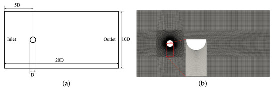
Figure 1.
(a) The computational domain ( m) and (b) the numerical mesh. The numerical mesh contains 171,864 points, 341,532 faces (169,668 internal faces), 85,200 cells, and 7 boundary patches, and the cells are all hexahedrons.
The computational domain is divided into hexahedral structured mesh cells, and the mesh spacing near the cylinder surface is refined small enough for capturing the boundary layer features. The mesh is generated by ICEM and converted to the mesh format accepted by OpenFOAM using a conversion tool named fluentMeshToFoam.
As shown in Figure 1b, the numerical mesh contains 171,864 points, 341,532 faces (169,668 internal faces), 85,200 cells, and seven boundary patches, and the cells are all hexahedrons. The mesh near the cylinder wall region is refined to satisfy . At the same time, the wall functions, such as kqRWallFunction, epsilonWallFunction, and omegaWallFunction, are used to solve the turbulence variables at the boundary.
Table 1 shows the parameters for the flow past a circular cylinder (Re = 3900). The relevant parameters of turbulence model, i.e., k, and , are determined by empirical formulas.

Table 1.
The parameters for the flow past a circular cylinder (Re = 3900).
The OpenFOAM uses the finite volume method, and the numerical scheme is set in the file “system/fvSchemes”. The specific numerical scheme is set as follows; the ddtSchemes is Euler; the gradSchemes is Gauss linear; the laplacianSchemes is Gauss linear corrected; the interpolationSchemes is linear; the snGradSchemes are corrected; and the divSchemes contain Gauss upwind, Gauss linear, and bounded Gauss upwind.
The total simulation time of the case is 50 s, and the time step is variable and is determined by the Courant number, which satisfies .
3.2. The PRT Steam Dumping Process
Figure 2 shows the computational domain of the PRT steam dumping process, which is same with Wang et al. [12]. The geometric parameters and the location of the sampling points have been marked in the figure, and the geometric parameters are modeled according to the actual building size. The PRT consists of nozzle, the gas chamber, and the non-gas chamber.
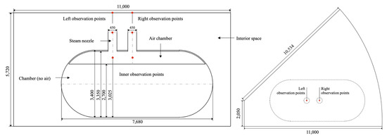
Figure 2.
Front and top views of the computational domain of the pressurizer relief tank (PRT) steam dumping process (all geometric parameters are in mm) [12]. There are 6 sampling points in the figure, 3 on the left and 3 on the right, which are, respectively, located inside the PRT, at the nozzle, and at the top of the shell. These points are represented by symbols as Lp-top, Lp-nozzle, Lp-inner, Rp-top, Rp-nozzle, and Rp-inner.
The computational domain of the steam dumping process of the PRT is divided into unstructured mesh shown in Figure 3. The mesh contains 573,583 points, 6,450,280 faces (6,286,476 internal faces), and 3,184,189 cells, which are tetrahedra. In the region close to the PRT, especially at the nozzle, the mesh is more dense than the region inside the shell. As in the case of flow past a circular cylinder, we use the wall functions such as kqRWallFunction, epsilonWallFunction, and omegaWallFunction to solve the turbulence variables at the boundary.
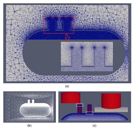
Figure 3.
The numerical mesh of the steam dumping process of the PRT, in which panel (a) is the mesh at the cross section, panel (b) is the overall grid, and panel (c) is the mesh detail of the gas chamber of the PRT. The mesh contains 573,583 points, 6,450,280 faces (6,286,476 internal faces), and 3,184,189 cells, which are tetrahedra.
The physical parameters of the case are divided into two parts. First, in the space inside the PRT, only the gas chamber is considered. The velocity is only 1 m/s in the z direction, the pressure is 1.6 MPa, and the temperature is 473 K (199.85 °C). Second, in the outer space of the PRT, the velocity is 0 m/s, the pressure is 0.1 MPa, and the temperature is 298 K (24.85 °C). Figure 4 shows the distribution of velocity, pressure, and temperature in the initial state.
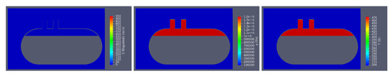
Figure 4.
The distribution of velocity, pressure, and temperature in the initial state. In the space inside the PRT, the velocity is only 1 m/s in the z direction, the pressure is 1.6 MPa, and the temperature is 473 K (199.85 °C), and in the outer space of the PRT, the velocity is 0 m/s, the pressure is 0.1 MPa, and the temperature is 298 K (24.85 °C).
Table 2 shows the steam parameters in PRT, and there are many thermodynamic parameters including Sutherland coefficient , specific heat capacity , and enthalpy change .
Table 2.
The parameters for the PRT steam dumping process.
The numerical scheme of the PRT steam dumping process is set as follows. The ddtSchemes are backward; the gradSchemes are Gauss linear; the laplacianSchemes are Gauss linear corrected; the interpolationSchemes are linear; the snGradSchemes are corrected; and the divSchemes contain Gauss upwind, Gauss linear, and Gauss linearUpwind Gauss linear.
The total simulation time of the case is 0.02 s, the time step is 5 × 10 −7 s, and the flow field physical quantity is saved every 1 × 10 −3 s.
In addition to the above physical model, the following basic assumptions are adopted in the calculation of this case. (1) It is assumed that the room of the PRT is a closed space with no physical quantity exchange with the outside world. (2) The influence of PRT internal structure on the flow field is ignored. (3) The nitrogen components in the gas space of the PRT are not considered in the calculation, and it is assumed that the gas space is full of water vapor and saturated under the initial state of the PRT. (4) Local condensation that may occur during pressure relief is not considered.
4. Results and Discussion
This paper carries out the numerical simulation on the high-performance computing platform of the State Key Laboratory of High Performance Computing. This platform has hundreds of computing nodes, each of which contains two Inter Xeon E5-2620 processors (6 cores, 2.10 GHz).
4.1. Flow Past a Circular Cylinder (Re = 3900)
In the case of flow past a circular cylinder, the Reynolds number is set to 3900. At this stage, the vortex street gradually transforms from laminar state to turbulent state.
The following is a comparative analysis of wake morphology, time history of lift coefficient (), drag coefficient (), pressure coefficient on cylinder surface, and mean stream-wise velocity and Reynolds shear stress in wake region.
Figure 5 shows the wake morphology (velocity contour map) of the three different turbulence models at the moment when the wake vortex is about to drop off the cylinder simulated by PRTFOAM. The three turbulence models all have wake vortexes behind the cylinder, and the wake vortex street is obvious. The wake morphology is similar with only slight differences. Figure 6 shows the wake morphology of the SSTKW model in one cycle. It is obvious that the vortex street is moving backwards.
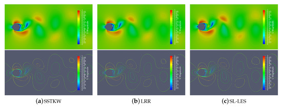
Figure 5.
The wake morphology (velocity contour map) of the (a) SSTKW model, (b) LRR model, and (c) Smagorinsky–Lilly SGS model-based LES (SL-LES) model at the moment when the wake vortex is about to drop off the cylinder simulated by PRTFOAM. It shows that the results of the three models all produce obvious vortex street behind the cylinder, with only slight differences in wake morphology. Moreover, SL-LES model is better at capturing small vortices.
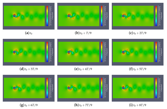
Figure 6.
The wake morphology of the SSTKW model in one cycle ( s), and subfigure (a–i) correspond to wake morphology at different times with interval s. It is obvious that the vortex street is moving backwards.
Combined with velocity contour map, it is easier to observe the differences in wake morphology of different models. The differences between different models will be analyzed and discussed with specific numerical results below.
When the fluid flows through the cylinder, it will produce the force of lift and drag of cylinder. From the beginning of simulation to the formation of stable vortex street, the time required decreases according to the order of SSTKW, LRR, and SL-LES models. The transition time of SSTKW model is the longest and SL-LES model is the shortest. Compared with the simulation results of commercial software CFX, the lift and drag coefficient is smaller than that of OpenFOAM, while for the LRR model, CFX’s solution of the wall boundary layer is not accurate enough to simulate the phenomenon of wake vortex shedding.
Table 3 lists the value of drag coefficient () and the value of Strouhal number () in each turbulence model, and compares them with Khan’s experimental values [32]. The frequency of vortex shedding directly affects the Strouhal number. In addition to the LRR model in CFX, the Strouhal number in other models is consistent with the experimental values.
Table 3.
The value of drag coefficient (), the value of Strouhal number () in each turbulence model, and the relative error with Khan’s experimental values [32].
In order to conduct a better analysis with specific numerical results, we sample in the wake region. The sampling diagram includes the measurement of the center line and vertical line behind the cylinder and the measurement of the angle on the surface of the cylinder, as shown in Figure 7.
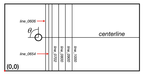
Figure 7.
Sampling diagram. The name of the vertical line corresponds to its x coordinate, for example, line_0606 means .
Figure 8 shows the pressure distribution around the cylinder surface including our numerical simulation data, the DNS of Ma et al. [17], and Norberg’s experimental results [33]. Because the pressure coefficient of the surface of the cylinder is symmetrical relative to the center line, namely, the upper half circle is the same as the lower half circle, only the pressure coefficient from 0 to 180 degrees of the upper half circle is taken in the figure. Because the CFX LRR model cannot fully simulate vortex shedding, it has a large deviation from other models. Compared with other models, except the CFX LRR model, the CFX SSTKW model is smaller at the minimum value of the pressure coefficient. All the simulation results are slightly smaller than the experimental values, but they are consistent on the whole.
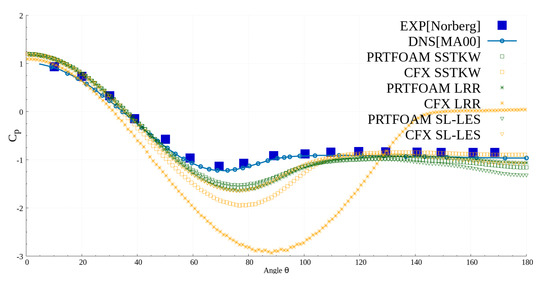
Figure 8.
The pressure coefficient from 0 to 180 degrees of the upper half circle. Because the CFX LRR model cannot fully simulate vortex shedding, it has a large deviation from other models. Compared with other models except the CFX LRR model, the CFX SSTKW model is smaller at the minimum value of the pressure coefficient.
Figure 9 shows the comparison of mean stream-wise velocity components at centerline behind the cylinder including our numerical simulation data; the DNS of Tremblay and Manhart [34]; and the experimental data of Lourenco and Shih [35], Ong and Wallace [36], and Beaudan and Moin [37]. In a distance behind the cylinder, the velocity shows a negative value, which means that in this distance, the velocity and the incoming flow are in the opposite direction, thus forming a back flow. Compared with the experimental results, the back flow length of numerical simulation is slightly smaller. It should be noted that the LRR model of CFX cannot simulate the phenomenon of vortex shedding, so its mean stream-wise velocity component is quite different from others.
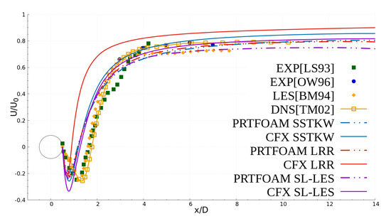
Figure 9.
Comparison of mean stream-wise velocity components at centerline behind the cylinder including our numerical simulation data, the direct numerical simulations (DNS) [34], and experimental data [35,36,37]. In a distance behind the cylinder, the velocity shows a negative value, which means that in this distance the velocity and the incoming flow are in the opposite direction, thus forming a back flow.
Figure 10 shows the comparison of mean stream-wise velocity components at vertical line behind the cylinder. Pay attention to the ordinate scale. By dividing the mean stream-wise velocity by the inlet velocity, the mean stream-wise velocity is normalized.
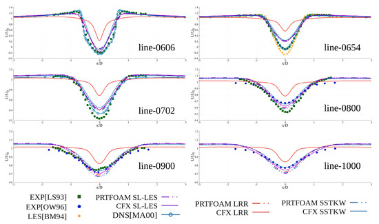
Figure 10.
Comparison of mean stream-wise velocity components at the vertical line behind the cylinder including our numerical simulation data, the DNS [17], and experimental data [35,36,37].
There are two convergence states about one diameter behind the cylinder, and the mean velocity profile shows two shapes, i.e., U-shape and V-shape. These two states are related to the width of the computational domain [17]. If the convergence states is U-shape in a certain computational domain, it will converge to V-shape for a wider computational domain. As there is only one computational domain of the case, there is one shape in the results. It can be seen from the subgraph line-0606 in Figure 10 that our results are consistent with the V-shape.
It is observed from the results that with increasing distance from the cylinder, the minimum value near the centerline is also increasing. The overall trend of the results is basically consistent with the experimental data, but the results of CFX’s LRR model have a large deviation.
Figure 11 shows the comparison of mean Reynold shear stress at vertical line behind the cylinder; also pay attention to the ordinate scale. Compared with other models, the amplitude of the simulation results of the SST k- model is slightly larger. Except for the CFX’s LRR model, the simulated values of other models are basically consistent with the experimental data.
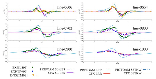
Figure 11.
Comparison of mean Reynold shear stress at the vertical line behind the cylinder including our numerical simulation data, the DNS [34], and experimental data [35,36].
In general, the simulation results of three models using OpenFOAM are better than CFX. The simulation results of the three models of OpenFOAM are similar, but the results of CFX are quite different, especially the LRR model.
4.2. PRT Steam Dumping Process
The PRT steam dumping process is a large-scale and complex engineering case. The steam with high pressure and temperature accelerates to supersonic speed instantly and ejects out from the nozzle, with the maximum speed reaching 972 m/s. The simulation results of different turbulence models are basically the same for the whole steam dumping process of the PRT. The SST k- model is taken as an example to describe the whole process. Then, according to the values of sampling points, the differences of simulation results of different models and different software are analyzed.
Figure 12, Figure 13 and Figure 14 show the velocity snapshots, pressure snapshots, and temperature snapshots of the simulation results of SST k- model with simulation time from s to s. From these figures, we can intuitively see that, driven by high temperature and high pressure, the steam in the PRT almost instantaneously accelerates to supersonic speed and ejects out from the nozzle. During the dumping process, the steam above the nozzle is maintained at a speed of 950 m/s. Until the steam reaches the top of the shell and spreads along the top, near the top of the shell, the speed of the steam drops sharply and the area covered by the high-speed steam continues to expand. In the whole process, the pressure in the PRT drops sharply, from 1.6 MPa at the beginning to approximately 1.2 MPa after 0.009 s, presenting an obvious gradual process. Consistent with common knowledge, the pressure in the left chamber near the nozzle is significantly lower than that in the right chamber away from the nozzle. The change in temperature is basically the same as the change in pressure. The difference is that the temperature of the top of the shell rises rapidly with the high-temperature steam dumping from the nozzle. At 0.009 s, it is close to the temperature of the steam inside the PRT. Therefore, the high temperature and impact should be fully considered in the top of the shell structure design of the top of the PRT.
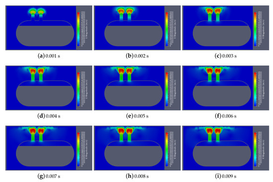
Figure 12.
The distribution of velocity of the simulation results of the SST k- model by using PRTFOAM at different times from (a) s to (i) s with interval s (legend unit: m/s).
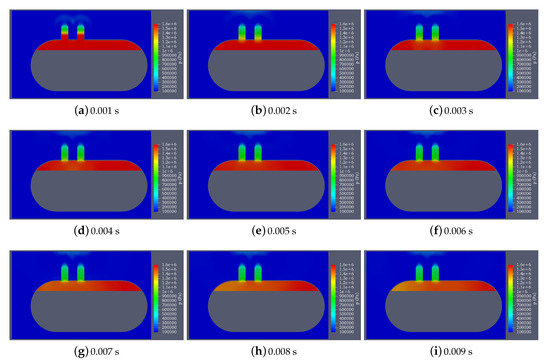
Figure 13.
The distribution of pressure of the simulation results of the SST k- model by using PRTFOAM at different times from (a) s to (i) s with interval s (legend unit: Pa).
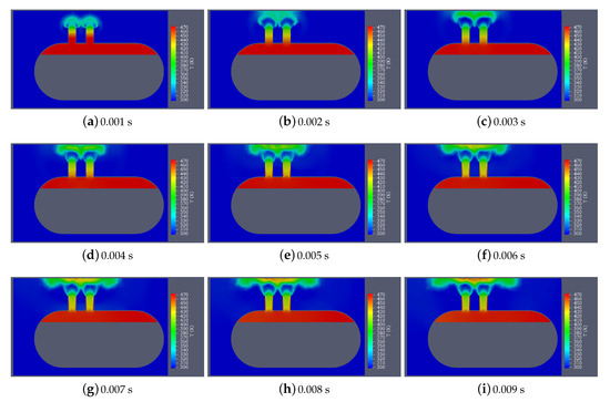
Figure 14.
The distribution of temperature of the simulation results of the SST k- model by using PRTFOAM at different times from (a) s to (i) s with interval s (legend unit: K).
At the beginning of the simulation, the difference between the internal pressure and external pressure of the PRT is up to 1.5 MPa, and the steam is ejects out through the nozzle, and its speed increases rapidly. When s, the steam velocity at the nozzle exceeds the speed of sound, reaching 760 m/s, but it has not had time to spread out, so the steam velocity at the nozzle is the largest in the whole domain. The flow direction of the steam is outward, and the steam inside the PRT is not affected. The steam generated by the PRT pushes the steam from the nozzle upward and spreads it. At the nozzle the pressure is 0.83 MPa, showing a gradual change.
At the time of 0.002 s, the steam has reached the top of the shell and begins to spread outward along the top. At this time, in the top area directly above the left steam nozzle, the steam velocity is up to 500 m/s, but it is not the largest in the whole domain. In the area between the nozzle and the top of the shell, the steam velocity is the largest, reaching 850 m/s. The pressure in the nozzle continues to drop as the steam is dumping. For the temperature distribution, the temperature in the area near the top of the shell reaches 380 K, but there is a low temperature area between the nozzle and the top because the steam moves at the fastest speed in this area, making it difficult to increase the temperature in a short time.
In the process of steam dumping, the pressure and temperature of the steam inside the PRT continue to decrease, while the velocity and temperature of the steam above the nozzle continue to increase, and eventually stabilize at a velocity of 950 m/s and a temperature of 450 K. The state distribution diagram at s can be regarded as a typical state. From this moment to the end of the simulation, the distribution of physical quantities changes only slightly but not dramatically.
Figure 15 shows the distribution of velocity, pressure, and temperature at the end of simulation ( s). At this time, the temperature and the pressure of the steam in the PRT gradually decreases to 458 K and 1.29 MPa, respectively. The results show that the simulation results of the three turbulence models are basically the same, and the process of steam dumping is the same as common sense. However, it is easy to find that the simulated results of LRR model show that at the same time ( s), the pressure and temperature in the chamber of the PRT are significantly higher than those of the other two models. At s, the simulated temperature of LRR is 464 K (190.85 °C), while that of other models is only 458 K (184.85 °C). Similarly, the simulated pressure of LRR is 1.41 MPa, while that of other models is only 1.29 MPa.
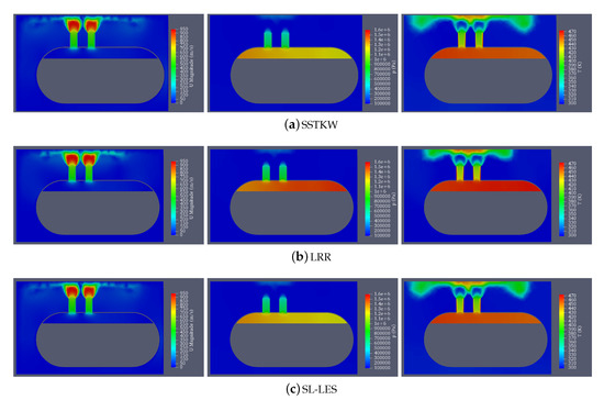
Figure 15.
The distribution of velocity, pressure, and temperature of the simulation results of (a) the SSTKW, (b) LRR, and (c) SL-LES model based on PRTFOAM at s. At this time, the temperature of steam in PRT gradually decreased to 458 K, and the pressure decreased to 1.29 MPa. The simulation results of the three turbulence models are basically the same, and the process of steam dumping is the same as common sense. However, the simulated results of LRR model show that at the same time, the pressure and temperature in the chamber of the PRT are significantly higher than those of the other two models. The simulated temperature of LRR is 464 K (190.85 °C), while that of other models is only 458 K (184.85 °C). Similarly, the simulated pressure of LRR is 1.41 MPa, while that of other models is only 1.29 MPa.
For a large-scale and complex engineering case, OpenFOAM shows more power than commercial software CFX. The numerical simulation of the three turbulence models based on OpenFOAM can all converge, while the CFX only SST k- model can successfully carry out numerical simulation. The following is a contrastive analysis of the simulation results of different turbulence models and different simulation software according to the velocity, pressure, and temperature obtained at the sampling point. Refer to Figure 2 for the position of the sampling point.
In order to compare the simulation results of the SL-LES model in the near-wall region, we add the simulation results of WALE model [20] in the comparison of results below, which solves the instability of eddy viscosity in a more natural way.
Figure 16 shows the pressure–time curves of the simulation results of different models at Lp-top and Rp-top sampling points. The high-pressure gas will directly impact the ceiling of the building and generate a strong impact load during the steam dumping process, which may have a certain adverse effect on the upper concrete structure. From the figure, we can get that when s, the pressure at the top of the shell increases from 0.1 MPa to 0.49 MPa instantly, and then gradually stabilizes at ~0.4 MPa. Compared with different models, the simulated dumping process of LRR model is significantly slower than that of other models, and the pressure at the top of the shell begins to surge at s. On the other hand, there is a problem in the pressure of the top shell simulated by commercial software CFX, that is, there is a large gap between the data of the left and right sampling point. The pressure on the left side is stable at approximately 0.4 MPa, which is consistent with other models. However, the pressure on the right side is finally stable at approximately 0.25 MPa, which is quite different from other models, and does not conform to common sense.
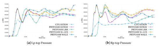
Figure 16.
Pressure–time curves of the simulation results of different models at the (a) Lp-top and (b) Rp-top sampling points. The simulated dumping process of LRR model is significantly slower than that of other models. There is a large gap between the data of the left and right sampling point simulated by commercial software CFX.
Figure 17 shows the temperature–time curves of the simulation results of different models at Lp-top and Rp-top sampling points. Different from the pressure, the temperature at the top shell increases gradually and stabilizes at approximately 450 K at s. It is worth noting that the temperature fluctuation of the Rp-top sampling point is significantly larger than that of Lp-top, and the simulation result of PRTFOAM LRR has a large deviation.
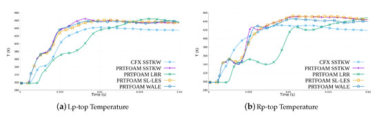
Figure 17.
Temperature–time curves of the simulation results of different models at the (a) Lp-top and (b) Rp-top sampling point. The temperature at the top of the shell increases gradually and stabilizes at approximately 450 K at s. The temperature fluctuation of the Rp-top sampling point is significantly larger than that of Lp-top, and the simulation result of PRTFOAM LRR has a large deviation.
Figure 18 shows the pressure–time curve and temperature–time curve of the simulation results in different models at the Lp-inner and Rp-inner sampling point inside the PRT, in which the curves of PRTFOAM SSTKW, PRTFOAM SL-LES, and PRTFOAM WALE basically coincide. The results show that the pressure and temperature inside the chamber of PRT decreases gradually and the relief effect is good. After s, the pressure in the air chamber decreased from 1.6 MPa to 1.29 MPa, and the temperature decreased from 473 K (199.85 °C) to 458 K (184.85 °C). The simulated dumping process of PRTFOAM LRR is slower than that of other models, and the pressure and temperature begin to decrease after 0.004 s, while other models begin to decrease after 0.002 s, and the pressure decline speed of PRTFOAM LRR is also significantly slower than that of other models. Except for PRTFOAM LRR, the simulation results of other models are basically consistent.
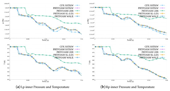
Figure 18.
Pressure–time curve and temperature–time curve of the simulation results of different models at the (a) Lp-inner and (b) Rp-inner sampling point inside the PRT. The curves of PRTFOAM SSTKW, PRTFOAM SL-LES, and PRTFOAM WALE basically coincide. The simulated dumping process of PRTFOAM LRR is slower than that of other models.
Figure 19 shows the velocity–time curve of the simulation results in different models at the Lp-inner and Rp-inner sampling point inside the PRT, and the curves of PRTFOAM SSTKW, PRTFOAM SL-LES, and PRTFOAM WALE are basically coincident. The velocity of the sampling point on the left side is stable at approximately 45 m/s, while that of the sampling point on the right side is stable at approximately 50 m/s. At the same time, the velocity of the observation point on the right side has an extreme value near s. At this time, the velocity reaches 70 m/s.
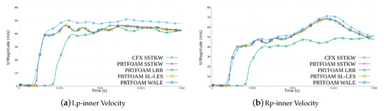
Figure 19.
Velocity–time curves of the simulation results of different models at the (a) Lp-inner and (b) Rp-inner sampling points. The curves of PRTFOAM SSTKW, PRTFOAM SL-LES, and PRTFOAM WALE basically coincide. The velocity of the sampling point on the left side is stable at approximately 45 m/s, while that of the sampling point on the right side is stable at approximately 50 m/s.
Figure 20 shows the velocity–time curve of the simulation results of different models at the Lp-nozzle and Rp-nozzle sampling point inside the PRT. Although the nozzle is not the place with the highest velocity in the whole space, it is an important place to observe the steam dumping process. The results show that the velocity–time curves of the four simulation results are basically the same, the velocity at the nozzle gradually increases with the steam dumping process and finally stabilizes at approximately 600 m/s. Compared with other simulation results, the velocity of CFX SSTKW is slightly smaller after its stabilization, only 552 m/s.
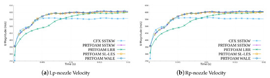
Figure 20.
Velocity–time curves of the simulation results of different models at the (a) Lp-nozzle and (b) Rp-nozzle sampling point. The curves of PRTFOAM SSTKW, PRTFOAM SL-LES, and PRTFOAM WALE basically coincide. The velocity at the nozzle gradually increases with the steam dumping process and finally stabilizes at approximately 600 m/s.
Through the above comparison, we found that the SST k- model and the Smagorinsky–Lilly SGS model-based LES approach are more appropriate than the LRR model for PRT simulations. Moreover, the open source solver PRTFOAM could be used to obtain better results than CFX in complex engineering cases. Only the SST k- model of CFX can converge to obtain simulation results, while the three models based on PRTFOAM can all converge. At the same time, there are some problems in the results of CFX SSTKW, that is, the pressure at the Lp-top and Rp-top sampling points is greatly different. Compared with different models, we found that the simulation results of the LRR model are not very ideal. First, the time of pressure and temperature drop during the steam dumping process lags behind that of other models, and second, the rate of pressure temperature drop is relatively slow. Fortunately, the results of the SST k- model and the results of the Smagorinsky–Lilly SGS model are generally consistent and desirable. However, the entire simulation time of the Smagorinsky–Lilly SGS model is almost twice as long as that of the SST k- model. This is why the RANS model based on the Reynolds average can still survive after the large eddy simulation (LES) is proposed.
5. Conclusions
Currently, numerical simulation has become a powerful tool for thermal hydraulics analysis in reactor structure and safety design. Due to the complex geometry of the full calculation domain and the turbulent flow characteristics of the compressible fluid from a PRT, it remains challenging to accurately simulate the transient flow dynamics during the steam dumping process.
In this study, we developed a compressible fluid solver PRTFOAM to numerically study the turbulent flow dynamics from a PRT. The PRTFOAM is implemented based on the OpenFOAM and designed to be capable of integrating various turbulence models. Two representative RANS models and the Smagorinsky–Lilly SGS model-based LES approach are coupled and tested in this solver. We first evaluated and analyzed the numerical solver PRTFOAM and the turbulence models using a benchmark case: flow past a circular cylinder (Re = 3900), and then the turbulent steam dumping process in the full geometry of a PRT is analyzed and compared with ANSYS CFX and literature reports. In addition, we tested the WALE model based on the PRT steam dumping process. The velocity–time, pressure–time, and temperature–time curves at selected sampling points have been compared in detail. The results show that the SST k- model and the Smagorinsky–Lilly SGS model-based LES approach are more appropriate than LRR model for PRT simulations. Moreover, it shows the simulation results of Smagorinsky–Lilly SGS model and WALE model are basically consistent under the condition of PRT steam dumping process. Under this condition, the drawbacks of the Smagorinsky–Lilly SGS model are not obvious. Furthermore, the comparison with CFX showed that our open source solver could be used to obtain better results in complex engineering cases. The design and testing results would provide guidance for further analysis of thermal-hydraulics in reactors based on open source codes.
However, we noticed that the computing efficiency of the open-source solver is obviously lower than the commercial software, which could be critical for simulating large scale applications. We plan to further analyze the parallel scalability of PRTFOAM on supercomputers and to study the performance optimizing techniques for engineering problems in thermal hydraulic transient analysis of nuclear reactors.
Author Contributions
Conceptualization, X.-W.G.; Data curation, S.Z.; Formal analysis, S.Z. and Y.L.; Funding acquisition, C.Y.; Investigation, R.Z.; Methodology, S.Z.; Project administration, C.Y.; Resources, X.-W.G. and C.L.; Software, S.Z., X.-W.G., C.L., Y.L. and R.Z.; Supervision, X.-W.G. and C.L.; Validation, S.Z.; Visualization, S.Z.; Writing—original draft, S.Z.; Writing—review & editing, X.-W.G. All authors have read and agreed to the published version of the manuscript.
Funding
This work was supported by the National Natural Science Foundation of China (Grant No. 61902413) and the open fund from the State Key Laboratory of High Performance Computing (No. 201901-12).
Acknowledgments
We would like to thank the anonymous reviewers for their time, work, and valuable feedback.
Conflicts of Interest
The authors declare no conflict of interest.
Appendix A
All symbols and acronyms used in this paper are summarized as follows.
Table A1.
The list of symbols and acronyms.
Table A1.
The list of symbols and acronyms.
| Symbol/Acronym | Meaning |
|---|---|
| PRT | Pressurizer Relief Tank |
| LWR | Light Water Reactors |
| PWR | Pressurized Water Reactors |
| DNS | Direct Numerical Simulation |
| RANS | Reynolds-averaged Navier-Stokes |
| LES | Large Eddy Simulation |
| Re | Reynolds number |
| SSTKW | the SST k- model proposed by Menter [24,25] |
| LRR | the Reynolds stress model based on Launder et al. [23] |
| SL-LES | the Smagorinsky–Lilly SGS model base LES approach [19,26] |
| SGS | Sub-grid-scale |
| Velocity | |
| Pressure | |
| Density | |
| Temperature | |
| () | components of velocity vector in x-, y- and z-direction |
| & | the source terms |
| the coefficient of thermal conductivity | |
| the dissipation function | |
| the second viscosity | |
| e | specific internal energy |
| specific heat capacity | |
| Reynolds stresses | |
| k | the turbulent kinetic energy |
| the dissipation rate of turbulent kinetic energy | |
| the specific dissipation rate | |
| the kinematic eddy viscosity | |
| the convective term | |
| the production term | |
| the rotational term | |
| the diffusion term | |
| the dissipation rate | |
| the pressure–strain term | |
| the SGS viscosity | |
| Sutherland coefficient | |
| enthalpy change | |
| reference temperature | |
| lift coefficient | |
| drag coefficient | |
| Strouhal number |
References
- Zvirin, Y. A review of natural circulation loops in pressurized water reactors and other systems. Nucl. Eng. Des. 1982, 67, 203–225. [Google Scholar] [CrossRef]
- Guo, X.W.; Xu, X.H.; Wang, Q.; Li, H.; Ren, X.G.; Xu, L.; Yang, X.J. A Hybrid Decomposition Parallel Algorithm for Multi-scale Simulation of Viscoelastic Fluids. In Proceedings of the 2016 IEEE International Parallel and Distributed Processing Symposium (IPDPS), Chicago, IL, USA, 23–27 May 2016; pp. 443–452. [Google Scholar] [CrossRef]
- Liu, Y.; Guo, X.W.; Li, C.; Yang, C.; Gan, X.; Zhang, P.; Wang, Y.; Zhao, R.; Fan, S. The Communication- Overlapped Hybrid Decomposition Parallel Algorithm for Multi-Scale Fluid Simulations. In Proceedings of the 48th International Conference on Parallel Processing. Association for Computing Machinery, Kyoto, Japan, 5–8 August 2019. [Google Scholar] [CrossRef]
- Zhang, J.; Shi, W.; Zhou, L.; Gong, R.; Wang, L.; Zhou, H. A Low-Power and High-PSNR Unified DCT/IDCT Architecture Based on EARC and Enhanced Scale Factor Approximation. IEEE Access 2019, 7, 165684–165691. [Google Scholar] [CrossRef]
- Baraldi, D.; Heitsch, M.; Wilkening, H. CFD simulations of hydrogen combustion in a simplified EPR containment with CFX and REACFLOW. Nucl. Eng. Des. 2007, 237, 1668–1678. [Google Scholar] [CrossRef]
- Hata, K.; Liu, Q.; Nakajima, T. Natural convection heat transfer from a vertical single cylinder with helical wire spacer in liquid sodium. Nucl. Eng. Des. 2019, 341, 73–90. [Google Scholar] [CrossRef]
- Zhang, Y.; Zhang, R.; Tian, W.; Su, G.H.; Qiu, S. Numerical prediction of CHF based on CFD methodology under atmospheric pressure and low flow rate. Appl. Therm. Eng. 2019, 149, 881–888. [Google Scholar] [CrossRef]
- Min Baek, S.; Cheon No, H.; Park, I.Y. A nonequilibrium three-region model for transient analysis of pressurized water reactor pressurizer. Nucl. Technol. 1986, 74, 260–266. [Google Scholar] [CrossRef]
- Qiang, G.; Yaodong, C. Hydrogen concentration distribution simulation during severe accidents in pressurizer relief tank compartment on NPP containment. At. Energy Sci. Technol. 2012, 46, 32–36. [Google Scholar]
- Gong, A.C.; Zhang, B.; Gao, Y.F. Thermal Design and Calculation of Pressurizer Relief Tanks. J. Chin. Soc. Power Eng. 2012, 7, 577–580. [Google Scholar]
- Wang, X.; Wang, M.; Zhang, J.; Wu, Y.; Tian, W.; Su, G.; Qiu, S. Study on the water seal formation process in advanced PWR pressurizer using CFD method. Ann. Nucl. Energy 2020, 135, 106949. [Google Scholar] [CrossRef]
- Wang, Y.; Guo, X.W.; Liu, D.; Wu, G.; Li, C.; Chen, L.; Zhao, R.; Yang, C. A 3D Numerical Study of Supersonic Steam Dumping Process of the Pressurizer Relief Tank. Energies 2019, 12, 2276. [Google Scholar] [CrossRef]
- Zou, S.; Yuan, X.F.; Yang, X.; Yi, W.; Xu, X. An integrated lattice Boltzmann and finite volume method for the simulation of viscoelastic fluid flows. J. Non-Newton. Fluid Mech. 2014, 211, 99–113. [Google Scholar] [CrossRef]
- Xu, C.; Deng, X.; Zhang, L.; Fang, J.; Wang, G.; Jiang, Y.; Cao, W.; Che, Y.; Wang, Y.; Wang, Z.; et al. Collaborating CPU and GPU for large-scale high-order CFD simulations with complex grids on the TianHe-1A supercomputer. J. Comput. Phys. 2014, 278, 275–297. [Google Scholar] [CrossRef]
- Giacomelli, F.; Biferi, G.; Mazzelli, F.; Milazzo, A. CFD modeling of the supersonic condensation inside a steam ejector. Energy Procedia 2016, 101, 1224–1231. [Google Scholar] [CrossRef]
- Sirisup, S.; Karniadakis, G.; Saelim, N.; Rockwell, D. DNS and experiments of flow past a wired cylinder at low Reynolds number. Eur. J. Mech.-B/Fluids 2004, 23, 181–188. [Google Scholar] [CrossRef]
- Ma, X.; Karamanos, G.S.; Karniadakis, G. Dynamics and low-dimensionality of a turbulent near wake. J. Fluid Mech. 2000, 410, 29–65. [Google Scholar] [CrossRef]
- Boussinesq, J. Theorie de l’ecoulement tourbillant. Mem. Acad. Sci. 1877, 23, 46. [Google Scholar]
- Smagorinsky, J. General circulation experiments with the primitive equations: I. The basic experiment. Mon. Weather. Rev. 1963, 91, 99–164. [Google Scholar] [CrossRef]
- Nicoud, F.; Ducros, F. Subgrid-scale stress modelling based on the square of the velocity gradient tensor. Flow Turbul. Combust. 1999, 62, 183–200. [Google Scholar] [CrossRef]
- Deardorff, J.W. A numerical study of three-dimensional turbulent channel flow at large Reynolds numbers. J. Fluid Mech. 1970, 41, 453–480. [Google Scholar] [CrossRef]
- Komen, E.; Camilo, L.; Shams, A.; Geurts, B.J.; Koren, B. A quantification method for numerical dissipation in quasi-DNS and under-resolved DNS, and effects of numerical dissipation in quasi-DNS and under-resolved DNS of turbulent channel flows. J. Comput. Phys. 2017, 345, 565–595. [Google Scholar] [CrossRef]
- Launder, B.E.; Reece, G.J.; Rodi, W. Progress in the development of a Reynolds-stress turbulence closure. J. Fluid Mech. 1975, 68, 537–566. [Google Scholar] [CrossRef]
- Menter, F.R. Two-equation eddy-viscosity turbulence models for engineering applications. AIAA J. 1994, 32, 1598–1605. [Google Scholar] [CrossRef]
- Menter, F.R. Eddy viscosity transport equations and their relation to the k-ε model. J. Fluids Eng. 1997, 119, 876–884. [Google Scholar] [CrossRef]
- Lilly, D.K. On the application of the eddy viscosity concept in the inertial sub-range of turbulence. NCAR Manuscr. 1966, 123. [Google Scholar] [CrossRef]
- Yakhot, V.; Orszag, S.A. Renormalization group analysis of turbulence. I. Basic theory. J. Sci. Comput. 1986, 1, 3–51. [Google Scholar] [CrossRef]
- WILCOX, D. Progress in hypersonic turbulence modeling. In Proceedings of the 22nd Fluid Dynamics, Plasma Dynamics and Lasers Conference, Honolulu, HI, USA, 24–26 June 1991; p. 1785. [Google Scholar]
- Menter, F.R.; Kuntz, M.; Langtry, R. Ten years of industrial experience with the SST turbulence model. Turbul. Heat Mass Transf. 2003, 4, 625–632. [Google Scholar]
- Patankar, S.V.; Spalding, D.B. A calculation procedure for heat, mass and momentum transfer in three-dimensional parabolic flows. In Numerical Prediction of Flow, Heat Transfer, Turbulence and Combustion; Elsevier: Amsterdam, The Netherlands, 1983; pp. 54–73. [Google Scholar]
- Issa, R.I. Solution of the implicitly discretised fluid flow equations by operator-splitting. J. Comput. Phys. 1986, 62, 40–65. [Google Scholar] [CrossRef]
- Khan, N.B.; Jameel, M.; Badry, A.B.B.M.; Ibrahim, Z.B. Numerical study of flow around a smooth circular cylinder at Reynold number = 3900 with large eddy simulation using CFD code. In Proceedings of the ASME 2016 35th International Conference on Ocean, Offshore and Arctic Engineering. American Society of Mechanical Engineers, Busan, Korea, 19–24 June 2016. [Google Scholar]
- Norberg, C. An experimental investigation of the flow around a circular cylinder: Influence of aspect ratio. J. Fluid Mech. 1994, 258, 287–316. [Google Scholar] [CrossRef]
- Tremblay, F.; Manhart, M.; Friedrich, R. LES of flow around a circular cylinder at a subcritical Reynolds number with cartesian grids. In Advances in LES of Complex Flows; Springer: Berlin/Heidelberg, Germany, 2002; pp. 133–150. [Google Scholar]
- Lourenco, L.; Shih, C. Characteristics of the plane turbulent near wake of a circular cylinder: A particle image velocity study (private communication), reported by Kravchenko, AG, Moin, P., 2000. Numerical studies of flow over a circular cylinder at ReD = 3900. Phys. Fluids 1993, 12, 403–417. [Google Scholar]
- Ong, L.; Wallace, J. The velocity field of the turbulent very near wake of a circular cylinder. Exp. Fluids 1996, 20, 441–453. [Google Scholar] [CrossRef]
- Beaudan, P.; Moin, P. Numerical Experiments on the Flow Past a Circular Cylinder At Sub-Critical Reynolds Number; Technical Report; Stanford Univ Ca Thermosciences Div: Stanford, CA, USA, 1994. [Google Scholar]
© 2020 by the authors. Licensee MDPI, Basel, Switzerland. This article is an open access article distributed under the terms and conditions of the Creative Commons Attribution (CC BY) license (http://creativecommons.org/licenses/by/4.0/).