Article

An Enhanced Vertical Ground Heat Exchanger Model for Whole-Building Energy Simulation

by
Matt S. Mitchell
1,* and
Jeffrey D. Spitler
2
1
National Renewable Energy Laboratory, Golden, CO 80401, USA
2
School of Mechanical and Aerospace Engineering, Oklahoma State University, Stillwater, OK 74078, USA
*
Author to whom correspondence should be addressed.
Energies 2020, 13(16), 4058; https://doi.org/10.3390/en13164058
Submission received: 26 June 2020 / Revised: 22 July 2020 / Accepted: 23 July 2020 / Published: 5 August 2020
(This article belongs to the Special Issue Design of Heat Exchangers for Heat Pump Applications)

Abstract

:
This paper presents an enhanced vertical ground heat exchanger (GHE) model for whole-building energy simulation (WBES). WBES programs generally have computational constraints that affect the development and implementation of component simulation sub-models. WBES programs require models that execute quickly and efficiently due to how the programs are utilized by design engineers. WBES programs also require models to be formulated so their performance can be determined from boundary conditions set by upstream components and environmental conditions. The GHE model developed during this work utilizes an existing response factor model and extends its capabilities to accurately and robustly simulate at timesteps that are shorter than the GHE transit time. This was accomplished by developing a simplified dynamic borehole model and then exercising that model to generate exiting fluid temperature response factors. This approach blends numerical and analytical modeling methods. The existing response factor models are then extended to incorporate the exiting fluid temperature response factor to provide a better estimate of the GHE exiting fluid temperature at short simulation timesteps.

1. Introduction

Whole-building energy simulation (WBES) programs, such as EnergyPlus® [1] and TRNSYS [2], use equipment-loop simulation algorithms that pass component (e.g., pumps, boilers, chillers, heat exchangers, etc.) entering and exiting conditions (e.g., flow rates, temperatures, humidity ratios, etc.) flow-wise from up-stream components to down-stream components. These components are generally connected in a loop so that every component on the loop is in some way connected to every other component on the loop. Equipment that is active at any given timestep may be controlled by an individual controller or by a larger control algorithm that specifies control for the entire system. These components may also make requests to other components for specific performance. For example, a chiller model that has a minimum required flow rate may require that all other components on the loop run at its minimum flow rate, even though they could be operated at a lower flow rate.
Passive equipment, on the other hand, simply operates by providing what it can at the current given conditions. For a ground heat exchanger (GHE), the models are only expected to be passed entering conditions, which in this case is the circulating fluid’s temperature and mass flow rate. As expected in the real world, the GHE will only give whatever performance it can physically deliver, regardless of what the other components on the loop require for successful operation. The objective of this study was to develop a GHE model that behaves in a similar passive manner, and to develop it for use in WBES environments. Requirements associated with this application are as follows.
First, the developed model must be accurate and produce physically realistic results. Some modeling simplifications may be necessary to meet secondary needs, such as simulation time. Regardless, the model should still produce a result that is as accurate as possible. In addition, WBES simulations often operate at non-uniform timesteps, so the model must accurately simulate GHE behavior at both short and long timesteps.
Second, the model should simulate GHE behavior as quickly and efficiently as possible. WBES simulations are often run on personal computers, such as laptops or desktop computers. These programs are generally not so sophisticated as to employ parallel- or multi-processing methods. Simulations are often run on a single computational process, which results in each sub-model within a WBES simulation being run in order, sequentially. Therefore, adding model complexity that significantly increases simulation time should only be done when absolutely necessary. Beyond this, modelers often use WBES to perform parametric analysis of designs, so any increase in simulation time has the potential to quickly amplify the total simulation time for any parametric study performed. This may be a challenge for designers who do not have access to a computer cluster.
Third, the model should be formulated to operate within a WBES environment. This means that the model should be formulated so the boundary conditions for the model can be clearly defined by the flow-wise upstream component and the external environment. For GHE, this implies that the GHE outlet fluid temperature can be computed directly from the inlet fluid’s temperature and mass flow rate as well as by other user-defined or environmental parameters. GHE thermal loads are not expected to be known before hand.
Fourth, the model should not rely on libraries, software, or other resources that are not freely available or that must exist external to the simulation environment. Historical WBES GHE models have relied on third-party libraries or software tools to provide input data for the simulation. To avoid this additional burden on the modeler, the model developed here must be able to operate in a standalone manner.

2. Literature Review

A number of different GHE modeling methodologies have been developed over the years. As is typical for methods and technologies that evolve with time, these models have evolved from simple, closed-form analytical expressions to methods that are mathematically complex and simulate specific, nuanced physical behavior. Several reviews of these models are presented in [3,4], but we review them again here in the context of WBES for completeness.

2.1. Analytical Models

Analytical models form the backbone of GHE simulation and validation and have been used extensively to model systems containing individual boreholes. Analytical models also provide an “exact” solution, which can be used to validate more complicated models.
Historically, GHE modeling methodologies have treated the region inside the borehole as separate from the region outside the borehole. Ignoring for a moment the U-tube, grout, and circulating fluid, the GHE may be thought of as a line or cylinder conducting heat into the ground, which is assumed to be a semi-infinite medium with a uniform, constant temperature and isotropic properties.
The infinite line-source (ILS) model is a pure conduction solution for an infinite line that conducts heat continuously at a constant rate into an infinite medium. Some authors have discussed who originally developed the method and the limits of its applicability [5,6,7,8]. Mogensen [9] applied several approximations to the method to compute the mean borehole fluid temperature. Spitler & Gehlin [6] provide a form of the method that is commonly used for thermal response test (TRT) analysis. The ILS form provided by Spitler & Gehlin computes the mean fluid temperature response results for a single borehole with constant heat input rate.
Infinite cylinder source (ICS) analytical models are similar to ILS models; however, the geometry is treated as a cylinder where varying conditions can be applied inside the cylinder. Three different forms have been given by Carslaw & Jaeger [7]. Solution methods for ICS solutions can be computationally expensive and some authors have provided methods to reduce this burden [10,11]. Others have developed ICS and ILS advancements for modeling ground water flow, ice formation, and helical geometries [11,12,13,14].
Finite line-source (FLS) models are another analytical solution method. Like ILS and ICS models, FLS models are relatively easy to compute but allow for the ground surface and GHE end effects to be taken into account. FLS models function by integrating point-source solutions over finite line segments. The individual temperature response of each segment is calculated based on its interactions with all other segments, and the temperature response of the GHE is determined by taking the average of the temperature responses of each segment in the GHE.
FLS models have been developed to model arbitrary GHE configurations, [15]; however, these can be computationally expensive, so simplified forms have also been developed [16,17]. FLS models have been validated against a 3D finite element model and integrated into GHE design tools [15,18,19].
While the analytical ILS and ICS methods described previously are useful for TRT analysis and for model validation purposes, they are not generally suitable for GHE simulation in the context of WBES. The methods assume an infinite ground medium, so end effects at the ground surface and bottom of the boreholes are not captured. These become more important over time, particularly in predicting long-term heat build-up or draw-down. The models also require temporal superposition to handle time-varying heat inputs, and even then are formulated to require heat input rather than entering fluid temperature inputs. ILS and ICS models also have limited accuracy at short times. FLS solutions are commonly used for computing response factors, which, as discussed in the next section, are useful for WBES.

2.2. Response Factor Models

Response factor models—commonly referred to as “g-function” models—are another commonly used model for simulating GHE performance. The so called “g-function” curves represent the non-dimensional temperature rise of the borehole vs. non-dimensional logarithmic time as seen in Figure 1.
These models apply Duhamel’s theorem [20,21], which posits that the time-varying temperature solutions to inhomogeneous, partial differential conduction equations can be solved in a piecewise fashion by applying step-pulse inputs. In other words, GHE temperature response due to time-varying heat inputs can be determined by applying the superposition of piecewise heat constant heat pulses. Claesson [22] began applying the principle of superposition to GHE modeling, and later, along with his Ph.D. student Eskilson [23,24,25], developed the response factor models commonly used today. The average borehole wall temperature can be computed for a single, constant heat pulse from Equation (1) or for a series of piecewise heat pulses as shown in Equation (2):
T b = T s + q 2 π k s * · g ( t / t s , r b / H , B / H , D / H )
T b = T s + i = 1 n q i q i 1 2 π k s * · g ( t n t i 1 t s , r b / H , B / H , D / H )
The g-functions are non-dimensionalized based on the characteristic time of the borehole field, t s = H 2 / 9 α s , where H is the borehole length and α s is the soil thermal diffusivity. D is the depth of the GHE below ground surface and B is the GHE center-to-center spacing.
As currently presented, response factor models are not useful for GHE simulation in the context of WBES without reformulation. The models are formulated in terms of known heat loads on the GHE, which creates a problem for WBES simulation because the GHE loads are not known a priori. Rather, the models are simulated at the same time as the other plant-loop components. The exiting fluid temperature and flow rate from one model is passed downstream to the next model, with all connected components affecting the performance of each other. As a result, the models need to be formulated in terms of known entering fluid conditions and not heat transfer loads. Additional methods also need to be applied to determine the circulating fluid heat transfer rate and associated temperature response instead of the temperature response at the borehole wall.
Response factor methods require that the GHE loads be accounted for from the beginning of the thermal history of the GHE. The result of this is that, as simulation time advances, the amount of effort required to compute the temperature response of the GHE continues to increase. Load aggregation procedures have been developed to mitigate these effects by collapsing loads that occurred far in the past relative to current simulation time be grouped together into one or more blocks. This helps to make response factor method simulation time more amenable to WBES programs. Mitchell & Spitler [26] have reviewed the available load aggregation methods and provided recommendations.
The traditional g-function formulation for short timesteps assumed that the fluid heat transfer rate, q f , and the borehole wall heat transfer rate, q b , are approximately equal. The result of this assumption is that the effective borehole wall temperature at short timesteps is negative, which is a non-physical value. Brussieux & Bernier [27] have shown that, as the timestep approaches 0, this value approaches 2 π k s R b . In the context of GHE modeling, “short timesteps” are timesteps that are shorter than the transit time of the GHE, which is the time it takes for the circulating fluid to transit through the GHE. Even for common GHE configurations, the transit time can range from minutes to tens of minutes. For a WBES program that can simulate timesteps down to 1 min, accurately computing the short-term transient effects is critical to accurately modeling GHE performance. As a result of these approximations, the outlet fluid temperature computed by the model can be non-physical when high loads are suddenly applied and the simulation timestep is small.
Several authors have modified the original response factor models to improve the short-term, dynamic accuracy of the model. Loveridge & Powrie [28] developed an addition to the original response factor model formulation for modeling concrete pile heat exchangers. The original model was modified by adding a “concrete response function” to account for the transient response of the pile heat exchanger. This method was successfully used to model pile heat exchangers with hourly loads; however, the method was not used for sub-hourly loads. The concrete response function was later used by Alberdi-Pagola [29] and Alberdi-Pagola et al. [30]; however, these studies also appear to be limited to hourly timesteps.
Pile heat exchangers are expected to be relatively short in length when compared to vertical borehole heat exchangers. As a result, the transit time of the circulating fluid from inlet to outlet is also expected to be lower. In addition, because sub-hourly timesteps are not expected, the above model is expected to perform well under these conditions. However, if the simulation timestep approaches the transit time, the model is expected to have trouble predicting the short-term dynamic response. This notwithstanding, the approach shows promise for the current application.
Others have directly computed g-functions for the purpose of directly predicting the GHE exiting fluid temperature. Dusseault & Pasquier [31] briefly mention the method, but a full derivation is given by Pasquier et al. [32]. The approach provides a way to utilize the Eskilson-type g-functions and combine them with the short-timestep g-functions for directly computing the fluid temperature. To compute these entering fluid temperature g-functions, a relatively complicated TRC model is utilized [33,34].
Finally, response factor methods require computing the response factors (i.e., g-functions) themselves. Claesson & Eskilson [23,25] created what is known as the superposition borehole model to generate g-functions. The heat transfer inside the borehole was assumed to be treated separately; therefore, the heat transfer rate computed by the model was from the borehole wall to the surrounding soil. There has been some discussion regarding what boundary conditions were applied at the borehole wall. Cimmino & Bernier [35] investigate this issue in detail by applying an FLS model and concluded that the model applies a uniform borehole wall temperature along the full length of the borehole, and that this temperature is uniform for all boreholes. Libraries of these g-functions representing specific GHE configurations have been published and used for GHE modeling; however, Malayappan & Spitler [36] point out that interpolation between these specific geometries can introduce errors.
ILS and ICS models may also be used to generate g-functions; however, because the internal geometry of the borehole is not considered and because of the various assumptions made regarding the thermal capacity of the borehole, ILS and ICS g-functions are not valid until after a certain time period, which can be up to several hours. Similarly, due to the infinite nature of the models, they will not be accurate at predicting periods when the GHE may interact with the ground surface.
FLS models are commonly used to generate g-functions. Cimmino & Bernier [35] developed a semi-analytical, discretized FLS model to generate response factors which is capable of simulating different borehole wall boundary conditions. Others have developed methods for computing response factors with series or parallel arrangements [16,37,38]. Cimmino [39] later developed a “fast” method for calculating g-functions that takes advantage of symmetry with the borefield to simplify and reduce computations. Cimmino later extended this model to compute g-functions for GHE with series- or parallel-connected boreholes [40,41]. The code for this library is published online [42].

2.3. Thermal Resistance-Capacitance Models

Thermal resistance-capacitance (TRC) models simulate the borehole internal geometry with a simplified resistance-capacitance network, as seen in Figure 2. These models can be formulated to solve for the heat transfer within the borehole by developing a network of temperature nodes that represent the temperature at different locations within the borehole. These temperature nodes are computed by defining an energy balance equation at each node. This energy balance generally also includes a transient term, which accounts for the thermal capacitance of the node. This allows the dynamic evolution of the node temperature over time to be determined.
This TRC approach has a benefit in that it does not require direct simulation of all of the geometry within the borehole (as would be done with pure numerical models that use finite-element or finite-volume methods). The result is that the temperature for each node can be solved for by simultaneously solving a set of equations, such as the example in Equation (3), where the left-hand side of the equation represents the transient temperature change with time and the right-hand side represents the energy flows between a node and its neighboring nodes:
ρ c p d T i t + Δ t d t = j = 1 n T j t T i t R i , j
Delta-circuit TRC resistance network models have been developed for single boreholes [43,44]. These models are coupled to several annular regions to complete a radial model of the borehole. The GHE is discretized vertically and multiple segments are stacked and connected which gives a quasi-2D representation of the borehole. Double U-tube and coaxial model configurations have been developed and validated against finite element numerical solutions [45]. Other authors have also added additional resistance-capacitance elements with the TRC model to improve the short-term transient behavior of the models [33,34,46,47].
Ruiz-Calvo et al. [48] describe what is potentially the most promising application of a TRC model for WBES applications. They use the TRC model to compute the heat transfer within the GHE, but then use a response factor model to update the borehole wall boundary temperature. This temperature is updated periodically so that the computations are only performed when needed.
TRC models are useful for representing additional physical detail for GHE modeling without the long simulation time or complexity required to solve a fully discretized numerical simulation. Unfortunately, the simulation time required to compute a TRC model is likely to be longer than would be acceptable for WBES programs. The model by Ruiz-Calvo et al. [46] required 20 s to solve for a 72-h TRT for a single borehole, whereas WBES simulations often run annual simulations of the entire building and connected systems within a similar amount of time. In addition to that, GHEs often need to be simulated for multiple decades to determine whether they have been sized appropriately. Therefore, a direct application of a TRC model within a WBES program would likely increase simulation time significantly, perhaps by several orders of magnitude. This would be considered unacceptable by designers who rely on WBES programs to perform rapid simulations for parametric analysis and design. TRC models are also more challenging to implement due to the complexity of the mathematical methods required. However, TRC models are quite useful for computing g-functions for short timesteps, near or below the transit time.

2.4. Numerical Models

Numerical methods, such as finite element or finite volume methods, have been applied to GHE modeling by several different authors. For example, Al-Khoury [49] developed two pure numerical solutions for modeling GHE. Shao et al. [50] apply these methods to develop a code base. Other pure numerical models have also been developed for simulating GHE performance [51,52,53,54,55]. They are often used as a validation method for other simplified models.
Direct numerical models that fully discretize the spatial domain using finite-volume or finite-element methods are useful for providing detailed results for model validation, but are not useful in the context of GHE modeling for WBES due to the excessive simulation time and inputs required to run such a model. Therefore, they are not considered further in this paper.

3. Methodology

Of the GHE modeling methodologies reviewed and discussed so far, only the response factor models are suitable for WBES applications because of their computational efficiency. This section outlines the development of an enhanced response factor model and discusses how it is used in WBES.

3.1. Enhanced Response Factor Model

Response factor models have been developed and used in WBES by Fisher et al. [56]. That model, which is based on the original formulation by Claesson & Eskilson [23,24], has functioned well; however, as noted previously, it can have trouble simulating short timesteps. So-called “short-timestep” response factors have been developed [27,57,58] to extend these limits, but non-physical behavior can still occur when the timestep is below the transit time.
The original response factor model is given in Equation (4) where the GHE load is used to compute the borehole wall temperature and the GHE mean fluid temperature is computed through a steady-state resistance value, as seen in Equation (5). The g-function values, g, are assumed to be computed at the appropriate time and GHE configuration as seen in Equation (6), where t n represents the simulation time of the current timestep:
T b = T s + i = 1 n q i q i 1 2 π k s · g
T f = T b + q n R b
g = f ( t n t i 1 t s , r b / H , B / H , D / H )
As presented above, this model is not suited for WBES because it requires the GHE load as an input parameter. However, these equations can be reformulated after assuming a relationship between the mean fluid temperature and the GHE inlet and outlet temperatures, and after assuming that the fluid heat transfer rate, q f , and the borehole wall heat transfer rate, q b , are equal. See Figure 3 for a simplified schematic of a borehole, with locations indicated for q f and q b . A full derivation of this reformulated model has been provided by Mitchell [59].
The approach adopted in this work may be considered a blend between the approach by Loveridge & Powrie [28] and Pasquier et al. [32]. Specifically, Loveridge & Powrie developed a response factor model with a separate g-function for modeling the short-term response of a concrete pile heat exchanger, and the model given by Pasquier et al. developed a way to combine the Eskilson-type g-functions with exiting fluid temperature g-functions for directly computing the exiting fluid temperature.
The proposed model is given in Equation (7). In this formulation, the GHE exiting fluid temperature is computed directly by modifying the historical response factor model (Equation (5)) with the addition of so called “exiting fluid temperature” (ExFT) response factors. These ExFT response factors are computed to determine the temperature difference of the GHE exiting fluid temperature from the borehole wall temperature. As a result, the model can be thought of as three individual parts, given in Equations (8)–(10). Part 1 (Equation (8)) computes the temperature difference between the borehole wall and the far-field soil; part 2 (Equation (9)) computes the temperature difference between the outlet fluid temperature and the borehole wall temperature; and part 3 (Equation (10)) computes the fluid heat transfer rate. All three parts are solved together simultaneously:
T o u t = T s + i = 1 n q i q i 1 2 π k s · g + R b i = 1 n ( q i q i 1 ) · g b
T b T s = i = 1 n q i q i 1 2 π k s · g
T o u t T b = R b i = 1 n ( q i q i 1 ) · g b
The first part comes from the historical response factor model. By applying this equation, the GHE borehole wall temperature difference from the soil temperature can be computed. The second part is the new formulation that computes the GHE exiting fluid temperature difference from the GHE borehole wall temperature.
To clarify, the heat transfer rate applied here is the calorimetric fluid heat transfer rate as calculated from the inlet and outlet temperatures as well as the flow rate of the GHE. This is seen in Equation (10), where T i n is the GHE entering fluid temperature and T o u t is the GHE exiting fluid temperature:
q f = m ˙ f c p , f H t o t ( T i n T o u t )
There are several reasons for formulating the model as shown:
  • Significant effort has been expended to understand and improve the original response factor model. Since its publication, researchers have performed many studies that enhance understanding of the methods and improve on the original work. This work similarly builds on the original model, about which much is already known, and which has already been widely adopted.
  • Because the formulation builds on the historical response factor model, software or other programs that already have this model implemented can more easily make modifications to incorporate the enhancements. This simplifies adoption of the model in WBES environments.
  • Again because the formulation builds on the historical response factor model, methods for generating standard borehole wall temperature g-functions are still applicable (as are load aggregation procedures, which are critical to maintaining low simulation times).
  • By clearly defining the heat transfer rate applied in this model as the fluid’s heat transfer rate, the domain inside the borehole and the domain between the borehole wall and the far-field soil temperature can be coupled together easily through two separate response factor computations. This more easily allows the transient effects to be handled, even down to timesteps below the transit time of the GHE circulation fluid.
The following section provides additional details about how the original and ExFT g-functions were developed and how the model is used in WBES.

3.2. Model Reformulation for WBES Usage

In order for the model to be applied in WBES, the model needs to be formulated from known quantities. In this case, we wish to pass an entering fluid temperature and mass flow rate to the GHE model and have it compute and return the exiting fluid temperature.
Starting with Equation (7), we will let Equation (11) apply, so the current model becomes that shown in Equation (12):
c 0 = 1 2 π k s
T o u t = T s + c 0 i = 1 n ( q i q i 1 ) · g + R b i = 1 n ( q i q i 1 ) · g b
To clarify, in response factor models, the multiplication of the heat rate differences by the g-function values is a convolution operation. For example, if three timesteps have occurred, the summation-convolution operation would be as follows:
i = 1 3 ( q i q i 1 ) · g = ( q 3 q 2 ) g ( t 3 t 2 t s ) + ( q 2 q 1 ) g ( t 3 t 1 t s ) + ( q 1 q 0 ) g ( t 3 t 0 t s )
Next, because the current heat load is not known, it is deconvolved from the response factor summations:
T o u t = T s + c 0 ( q n q n 1 ) · g n + c 0 i = 1 n 1 ( q i q i 1 ) · g + R b ( q n q n 1 ) · g b , n + R b i = 1 n 1 ( q i q i 1 ) · g b
For simplification, we will let the g-function values for the current heat load be noted as shown in Equations (15) and (16):
g n = g ( t n t n 1 t s )
g b , n = g b ( t n t n 1 t s )
From there, the historical terms are gathered together in Equation (17), which then leaves Equation (18):
c 1 = c 0 i = 1 n 1 ( q i q i 1 ) · g + R b i = 1 n 1 ( q i q i 1 ) · g b
T o u t = T s + c 0 ( q n q n 1 ) · g n + R b ( q n q n 1 ) · g b , n + c 1
After this, we apply another replacement to simplify the notation (Equation (19)), which then leaves Equation (20) after the current heat transfer rate, q n , and the previous timestep heat transfer rate, q n 1 , are gathered together:
c 2 = c 0 g n + R b g b , n
T o u t = T s + c 2 q n c 2 q n 1 + c 1
Because we wish to clearly define the model in terms of the fluid heat transfer rate, Equation (10) is again introduced in Equation (21), after another simplification is applied in Equation (22):
q f = c 3 ( T i n T o u t )
c 3 = m ˙ f c p , f H t o t
After Equation (21) is substituted into Equation (20) and after some algebraic manipulation, we arrive at the final solution in Equation (23):
T o u t = T s + c 2 c 3 T i n c 2 q n 1 + c 1 1 + c 2 c 3
The model is now cast in terms of known quantities. The question remains, though, regarding how to compute the g-function values. To do this, a simplified dynamic borehole model has been developed. This will be discussed in the next section, along with computation of the g-function values.

3.3. Dynamic Borehole Model

As discussed previously, this model can be considered a blend between the approaches outlined by Loveridge & Powrie [28] and Pasquier et al. [32]. In Loveridge & Powrie’s paper on pile heat exchangers, the authors used a detailed numerical model to compute the transient response [60]; in Pasquier et al.’s work on the borehole heat exchanger, a detailed TRC model was used to determine the short-term, dynamic response [33,34]. A similar approach will be taken here; however, because computation time is so important, a fast solution is desired.
To do this, a simple dynamic borehole model has been developed, which will be used to compute the ExFT g-functions. The model is composed of two simple, 1D dynamic pipe models for simulating the transit delays and a simple five-node TRC model for simulating heat transfer within the borehole. This is seen in Figure 4.

3.3.1. Simple Borehole TRC Model

A schematic of a segment of the simple TRC model borehole is shown in Figure 5. The model is a simple, five-node model. For comparison, the model used by Pasquier & Marcotte [34] has 16 nodes per segment with multiple segments stacked together. The number of segments used was left as a parameter that could be varied during model validation.
The resistance values are set using the first-order approximation of multipole method [61,62,63], where R b is the borehole thermal resistance and R 12 is the direct-coupling resistance. Javed & Spitler [64] discuss the accuracy of these methods and note that, in most situations, the first-order approximation is accurate to within 1%.
Equations for computing R b have been given in Javed & Spitler [64,65]. Direct-coupling resistances using the multipole method are not given in the literature, so it has been derived from the Delta-circuit resistance network and given in Equation (24) in terms of the borehole resistance and the total internal borehole resistance, R a (both of which can be computed directly from the multipole method). Fluid resistance in the flow direction is computed as shown in Equation (25):
R 12 = 4 R a · R b 4 R b R a
R f = 1 m ˙ f c p , f
Equations for computing the temperature of each of the temperature nodes from the borehole segment model are given below.
C f , 1 d T f , 1 d t = T i n , 1 T f , 1 R f , 1 + T g , 1 T f , 1 R 12 / 2 d z + T g , 2 T f , 1 R b d z
C f , 2 d T f , 2 d t = T i n , 2 T f , 2 R f , 2 + T g , 1 T f , 2 R 12 / 2 d z + T g , 3 T f , 2 R b d z
C g , 1 d T g , 1 d t = T f , 1 T g , 1 R 12 / 2 d z + T f , 2 T g , 1 R 12 / 2 d z
C g , 2 d T g , 2 d t = T f , 1 T g , 2 R b d z + T b T g , 2 R b d z
C g , 3 d T g , 3 d t = T f , 2 T g , 3 R b d z + T b T g , 3 R b d z
The thermal capacity for each node is set from the product of their respective heat capacity and volume. This is shown below for the fluid capacity elements, assuming equivalent pipe sizes for both pipes in the segment:
C f , 1 = ρ f c p , f V f , 1
C f , 2 = C f , 1
The grout capacity nodes are slightly different because it is difficult to determine what fraction of the total volume grout should be associated with each node. Therefore, this fractional value is included in the grout capacity nodes, which could be adjusted during model validation. Total grout volume can be determined by taking the total volume inside of the borehole and subtracting the total pipe volume:
C g , 1 = f g ρ g c p , g V g
C g , 2 = C g , 3 = ( 1 f g ) ρ g c p , g V g 2
Equations (26) through (30) are solved simultaneously using a Runge–Kutta fourth-order time integration scheme [66]. Model boundary conditions are the inlet temperatures and mass flow rates for each leg of the U-tube segment as well as the borehole wall temperature. All node temperatures are initialized to the undisturbed ground temperature.
The borehole wall boundary temperature is updated each timestep using the response factor calculation seen in Equation (4). g-function response factors are computed using the pygfunction library [42], which uses FLS methods for long-timestep g-functions [39]. Short-timestep g-functions are computed using the 1D, radial finite volume model developed by Xu & Spitler [58]. However, instead of using the model to evaluate the fluid temperature rise and then subtract the borehole resistance—which effectively results in a negative borehole wall temperature response at short timesteps—the actual borehole wall temperature rise is evaluated and then the short-timestep g-functions are computed.

3.3.2. Dynamic Pipe Model

In order to simulate the transit delay effects within the borehole, a dynamic pipe model is used. This dynamic pipe model was originally developed by Bishoff & Levenspeil [67] and later improved by Skoglund & Dejmek [68]. Rees [69] applied the model in a fashion similar to the current application, except the author used a 2D, radial-angular finite volume model to compute the heat transfer within the borehole. The model applies a single plug-flow element that tracks the history of the pipe inlet temperatures, then the temperature nodes along the pipe are mixed together in ideally stirred tank elements. Skoglund & Dejmek [68] recommend 16 elements to achieve a good balance between accuracy and performance. In the model applied here, only the plug-flow time delay is applied to the inlet pipe. The outlet pipe directly mixes the element temperatures together to determine the dynamic temperature response. Computing the temperature of the stirred elements can be accomplished with a tri-diagonal matrix inversion solution, often referred to as the Thomas Algorithm [66]. This convenient formulation allows the computations to execute quickly.
The model is limited to simulating turbulent flows; however, the present study also used the model for laminar flows, so addressing this is recommended for future work. Note that the general methods developed in this section for an enhanced response factor model are not dependent on this particular dynamic borehole model. Any dynamic model that computes the short-term, transient temperature response of the borehole could be used, assuming it is accurate and fast to compute.

3.3.3. Dynamic Borehole Model Validation

In order to validate the dynamic borehole model, a parametric study using the model was run and compared against experimental data collected by ourselves in 2014. The data were collected from two multi-flowrate thermal response tests (MFRTRT) where the heat input rate was held constant and the flow rate was varied at discrete intervals. The first "high" flow rate test varied the flow from 0.15 k g / s , to 0.30 k g / s , to 0.45 k g / s . This resulted in flows with Reynolds numbers of approximately 12k, 21k, and 32k, respectively. The second "low" flow rate test varied the flow from 0.02 k g / s to 0.2 k g / s in eight intervals. This resulted in flows with Reynolds numbers ranging from approximately 2.2k to 22k. Additional information regarding these tests is given by Beier et al. [70]. Parameters regarding the borehole configuration match those provided by Beier et al.
Because the dynamic borehole model is only expected to run long enough to generate the ExFT g-functions, the model was only run for 24 h using the GHE inlet conditions logged from the experimental data. The parameters varied in the study were the grout fraction, number of iterations, number of TRC model segments, and the simulation timestep. The results from the parametric study plot the simulation time required for exercising the model for a single flow rate on the vertical axis, and plot the root mean squared error of the exiting fluid temperature on the horizontal axis.
Figure 6 shows the data with the Pareto front identified. The Pareto front was identified using the “pareto” Python library [71], which employs the popular non-dominated sorting genetic algorithm NSGA-II [72].
The Pareto data are given in Table 1. The second configuration identified was then used to run the dynamic borehole model to simulate using additional data from the MFRTRT. The mean bias error is also given, which is the average exiting fluid temperature error. Even at 7.8 s , the time required to compute ExFT g-functions is acceptable for WBES. Note that the software used for this project was implemented in the Python programming language on a Windows 10 computer with a 3.4 G Hz processor. Python is not known for its computational speed, so these times could be improved significantly by implementing the code in a compiled programming language, such as C++.
Figure 7 shows the full nine days of the high-flow MFRTRT. The model is driven from the experimental measurements of the GHE inlet temperature and flow rate. The outlet temperature error is also plotted. Despite the dynamic borehole model being extremely simple, the results are promising. Some error associated with transit time computation is shown near the beginning of the test; however, the general trend of the model follows the experimental data well. For most of the first two hours, the exiting fluid temperature error is within 0.5 C .
Again, during most of the test, the exiting fluid temperature error is within 0.5 C , with the exception of the periods during the flow rate step-change. Again, these are caused by errors in the transit delay prediction.
Figure 8 shows the first two days of the low-flow MFRTRT. Some experimental interruptions occurred, which require some special treatment in order to apply the current model. Therefore, no additional comparisons are made beyond the two days shown. Exiting fluid temperature error is slightly higher than the high-flow MFRTRT.
Improvements could certainly be made to the dynamic borehole model; however, the model is sufficiently accurate for generating ExFT g-functions for the enhanced response factor model.

3.4. Exiting Fluid Temperature Response Factor Generation

To generate the ExFT g-functions, the simplified dynamic borehole model is exercised with a constant heat load and constant flow rate. Once the model is initialized, the flow rate is held constant and the inlet temperature is computed based a first-law energy balance for a fixed heat input rate. The dynamic borehole model exiting fluid temperature is then fed back into the inlet of the GHE after again applying a first-law energy balance for a fixed heat input rate. By exercising the model in this fashion, the transit delay effects can be estimated and incorporated into the g b values computed.
The temperature response data from the model is then converted to the ExFT g-function values and given for their respective non-dimensional time. The ExFT g-functions are computed as shown in Equation (35). Non-dimensional time that is used for response factor models is computed as shown in Equation (36):
g b = T E x F T T b q f · R b
ln ( t / t s ) = ln ( t H a v e 2 / ( 9 α s ) )
In Equation (35), the temperature difference and the heat transfer rate are expected to be proportional to one another, so the only changes expected in the resulting g b values computed will be due to the borehole resistance calculation. R b includes the pipe resistance, which will be affected by changes in flow rate and fluid temperature. Because R b can change significantly with the flow rate, it is expected that the flow rate values used for computing g b are not arbitrary, and that g b will need to be computed for multiple values in order to account for variations in flow rate.
Figure 9 shows the g b values which were computed plotted vs. non-dimensional time. As expected, higher flow rate data begin to increase sooner than low flow rate data due to the differences in the transit time from different flow rates. Undulations in the data are directly related to the transit delay effects. Excerpted data from the g b computations at t = 24 h are given in Table 2.
From the table, we can see that the fluid heat transfer rate is nearly constant. Additionally, the borehole resistance decreases with flow rate, except for the first flow rate of 0.02 kg/s which is 0.5% lower than the resistance at 0.03 kg/s. The cause of this is unknown at the moment but is likely attributable to differences in fluid property computations due to temperature differences. For reference, fluid properties were computed using the CoolProp thermophysical properties library [73]. The borehole wall temperature is also nearly constant as is expected because the heat transfer expected at the borehole wall should approach a steady value after enough time, regardless of the fluid flow rate.

3.5. Borehole Wall Temperature Response Factor Generation

Standard g-function values used for computing the borehole wall temperature rise could be computed in a number of ways. These have been discussed in the literature review and are not repeated here. The methods developed by Cimmino [39] will be used through the pygfunction Python library [42] for computing the long-timestep g-functions. Short-timestep borehole wall temperature g-functions are computed using the 1D radial finite-volume model developed by Xu & Spitler [58]. These g-functions are plotted in Figure 10 for the MFRTRT borehole discussed in Beier et al. [70]. Because it can be difficult to understand non-dimensional time values, some dimensional values are given as well.
As stated previously, the g-function values are evaluated to give the borehole wall temperature rise, not the fluid temperature rise. For this reason, the values approach 0 for lower ln ( t / t s ) values. The original implementation of the model by Xu & Spitler [58] subtracts the steady-state borehole resistance so the mean fluid temperature could be computed. Other short-timestep g-function generation methods do this as well; however, this is not correct for the current model’s formulation. As expected, some time is required for the heat to conduct from the fluid, through the grout, to the borehole wall. As seen in the plot, this time is on the order of 20–30 min for this particular borehole.
The model by Xu & Spitler [58] is a 1D, radial finite-volume model as outlined by Patankar [74], which is formulated to be solved using a tri-diagonal solution scheme. The solution is computed with a fixed timestep of 2 min for 24 h , after which the long-timestep g-function methods are applied.
As with the dynamic borehole model, the choice of flow rate will affect the short-timestep borehole wall g-functions. However, because we are evaluating the borehole wall temperature with a fixed heat input rate, the effect on the short-timestep g-functions is expected to be quite small, and therefore the choice of flow rate used to compute the short-timestep and long-timestep g-functions is arbitrary.

3.6. Methodology Summary and Discussion

The methods used in this enhanced model are similar to previous response factor models; however, the method has been modified to better compute the GHE exiting fluid temperature at short timesteps. To simplify, the methods described previously could be summarized and implemented as follows:
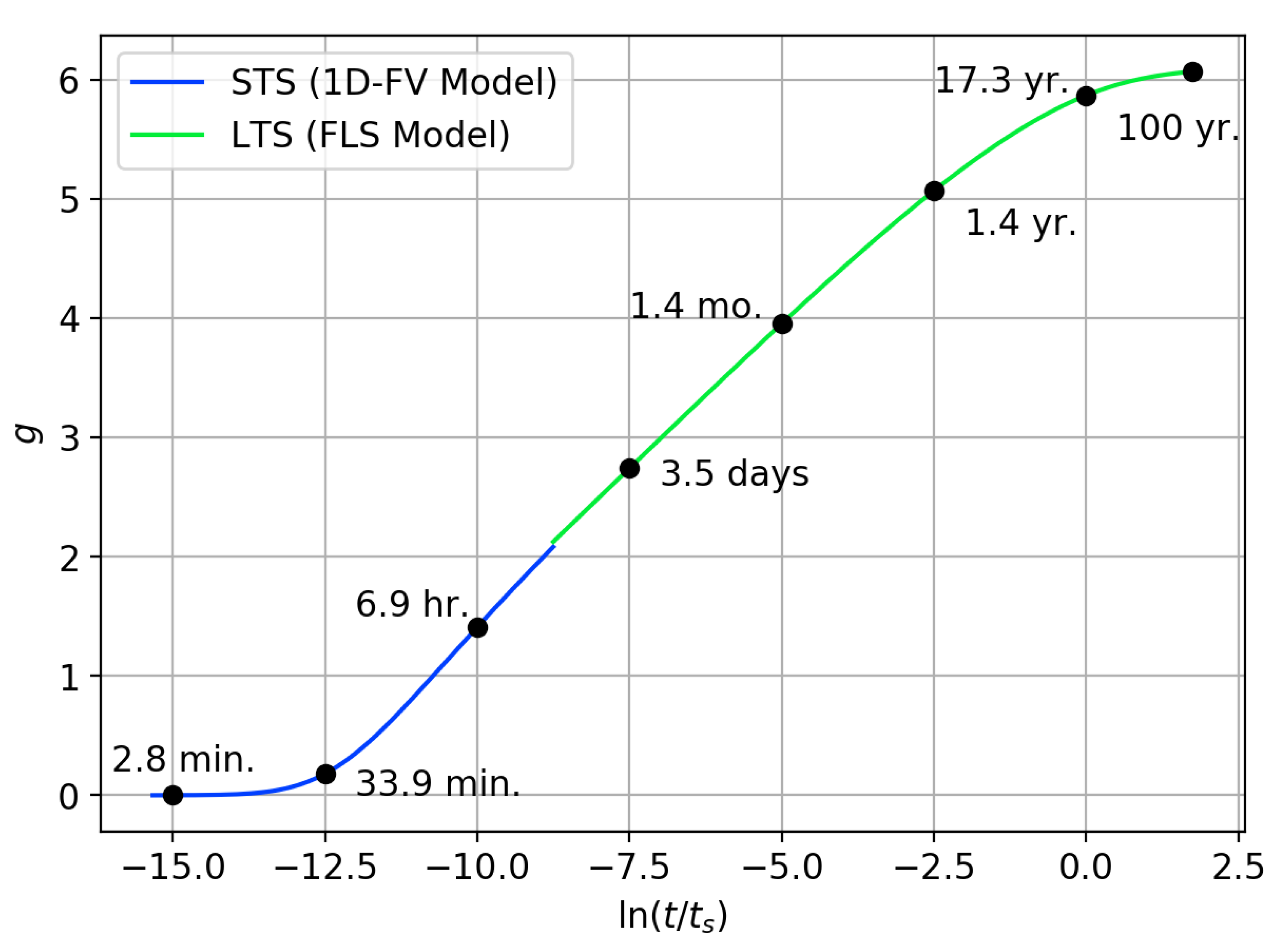
  • Long-timestep borehole wall temperature g-functions could be computed with any number of approaches outlined previously. In this work, an FLS approach was used by utilizing the pygfunction library by Cimmino [42]. No modifications are required to the methodology used to compute these g-functions. Cimmino has produced significant quantification regarding the speed of these methods [39] and has shown that for borefields with up to 64 boreholes—which is realistically expected to capture most of the WBES use cases—g-functions can be computed in times from a few seconds to a few minutes. Note that the code by Cimmino is written in Python; the computation time could likely be reduced to some extent after being implemented in a compiled programming language.
  • Short-timestep borehole wall temperature g-functions could also be computed using any accurate borehole model that captures the dynamic effects of the borehole thermal capacity on the borehole wall temperature. In this work, the model by Xu & Spitler [58] was used because it uses a simplified geometry that accounts for the borehole thermal capacity. In addition, it is a 1D, radial finite-volume model that can be solved rapidly using a tri-diagonal matrix formulation. Note that the original model has to be slightly modified to compute the temperature at the borehole wall, and not at the fluid. This model is highly efficient and can compute the short-timestep g-functions in a matter of seconds.
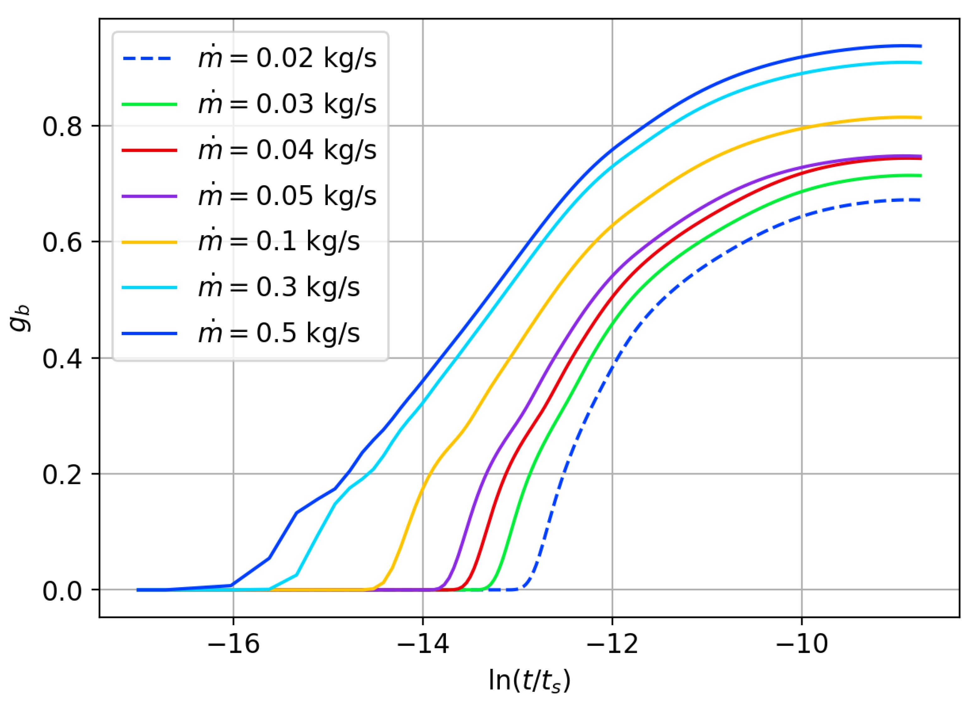
  • Exiting fluid temperatures g-functions are computed with a simplified dynamic borehole model that accounts for the transit delay of the circulation fluid via utilization of a transit delay pipe model. As before, the method presented in this paper does not rely on this specific dynamic GHE model; rather, any dynamic GHE model that accurately captures the transit delay effects of the borehole could be used, assuming that it is sufficiently fast and accurate. The borehole wall boundary temperature was updated by computing the heat flux at the borehole wall and then using that information to inform the original heat-input-formulated response factor model (Equation (4)). The borehole wall temperature resulting from that was then set as the borehole wall temperature boundary condition and updated at each timestep. Note that the short-timestep g-functions computed in the previous step are used here for determining the updated borehole wall boundary temperature. The dynamic model used here was able to compute the exiting fluid temperature g-functions for a single flow rate in 7.8 s , which is an acceptable time for WBES. Note that this should be repeated for different flow rates and that additional work should be done to determine how many different g b values are needed.
Though the method does require some computation time for the various required g-functions, these times are acceptable for WBES applications. Additionally, if the GHE configuration does not change, these values could be cached and stored for reuse during subsequent simulations. Provided that the GHE is not changed, these values do not need to be recomputed for each simulation.

4. Validation

The enhanced response factor model is validated using the MFRTRT data. Validation results for the high- and low-flow tests are presented in this section. For all cases, the experimental measurements for temperature and flow rate were used as the inlet conditions for the GHE model.

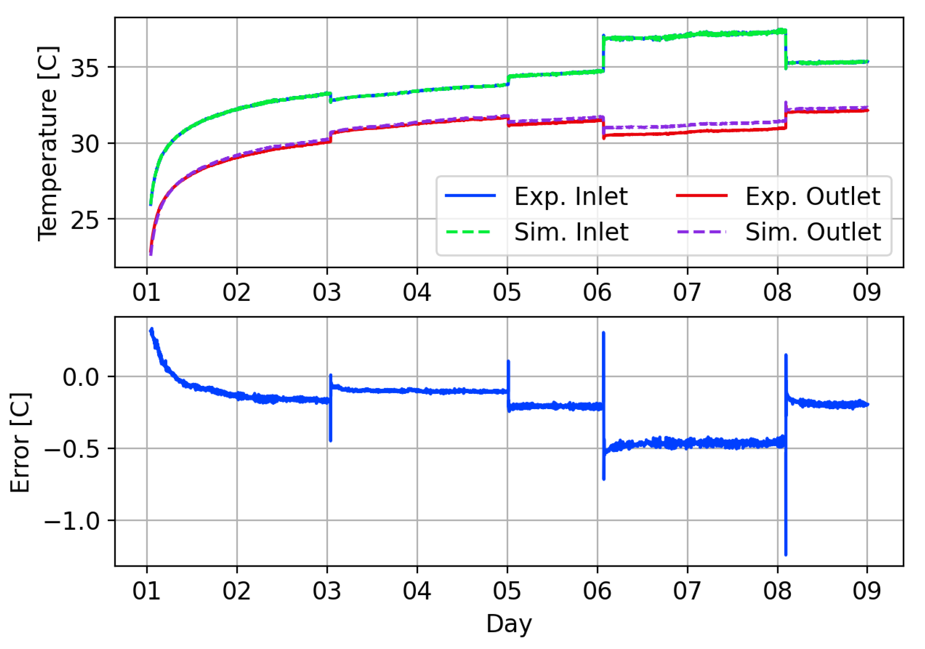
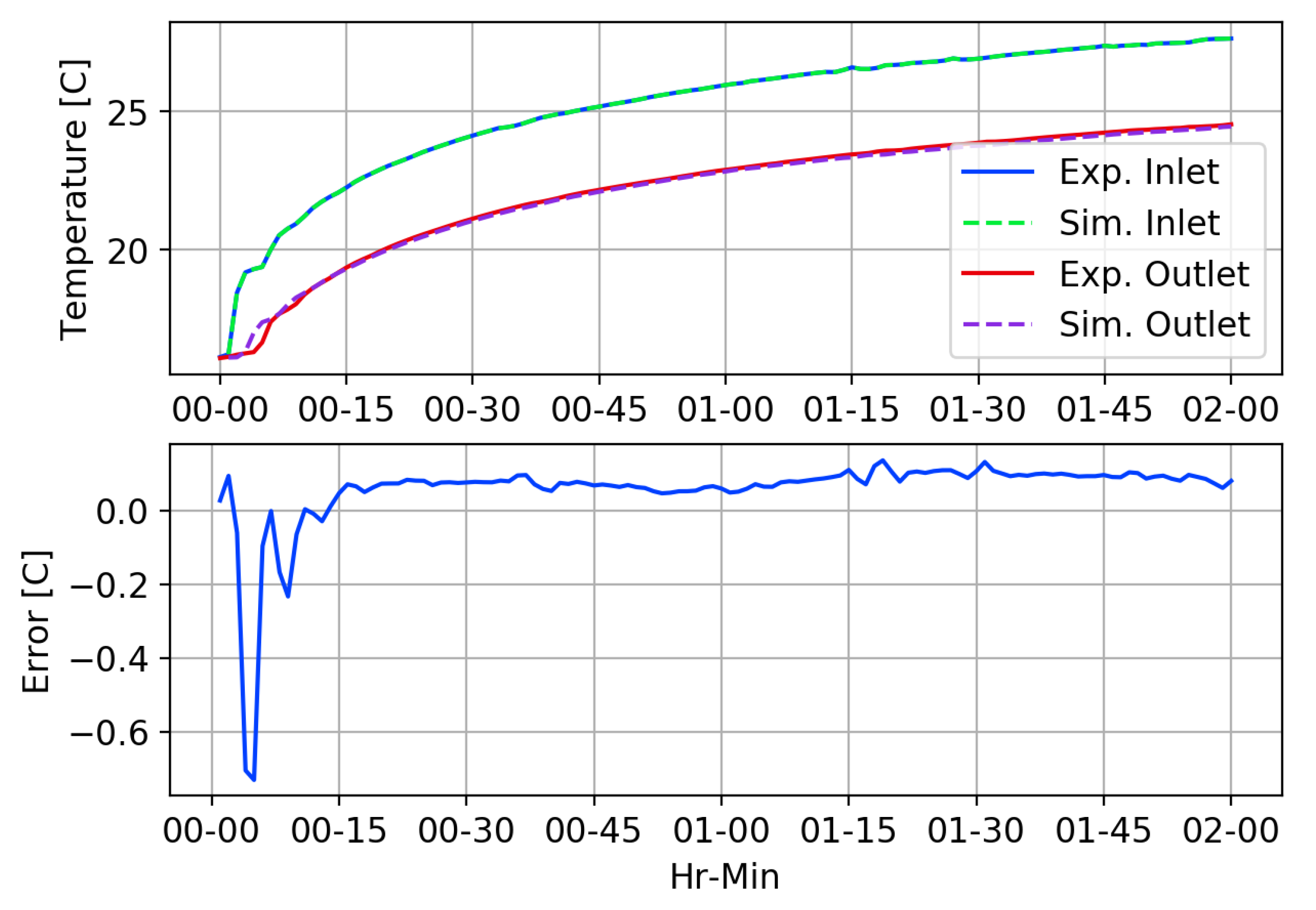
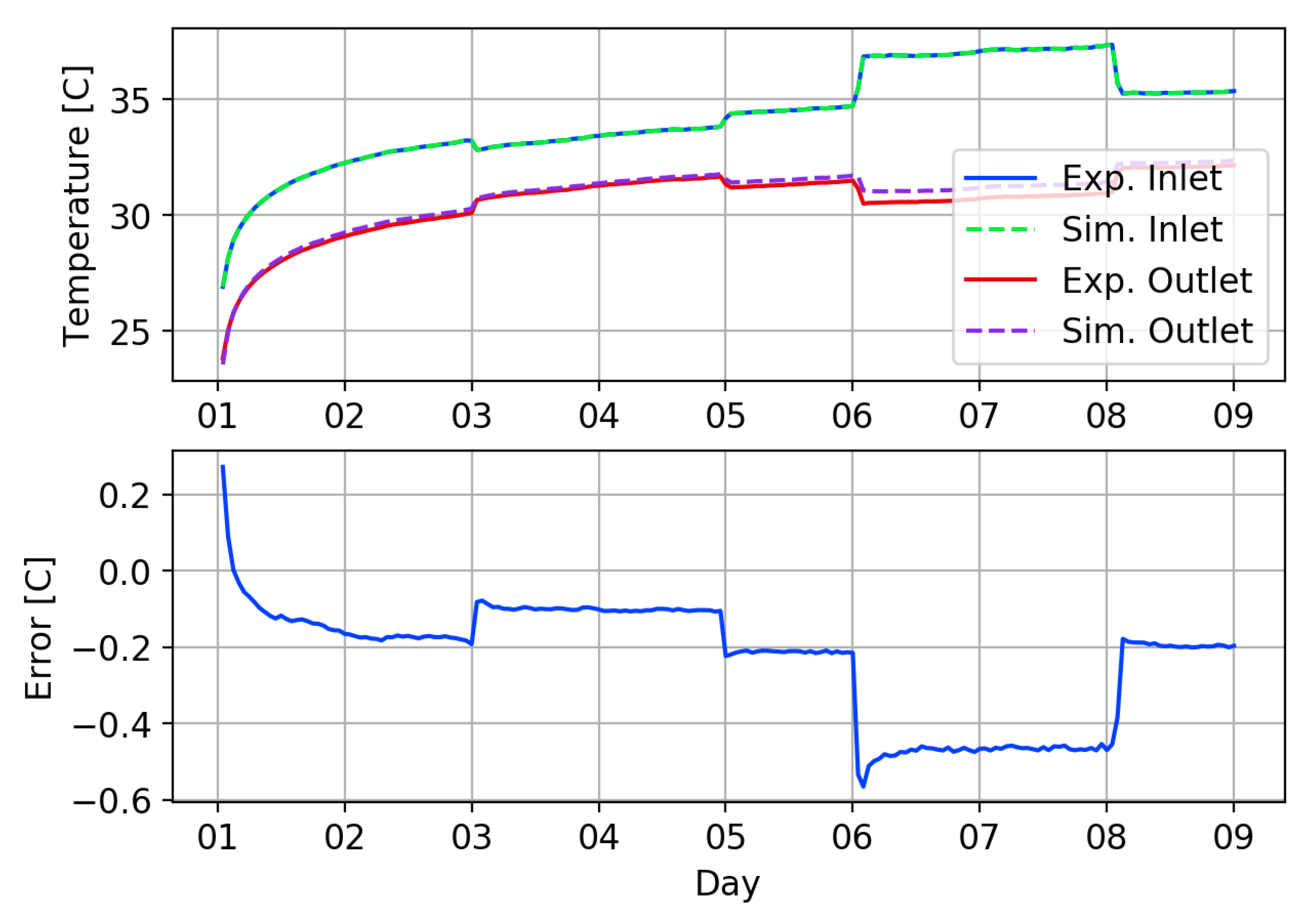
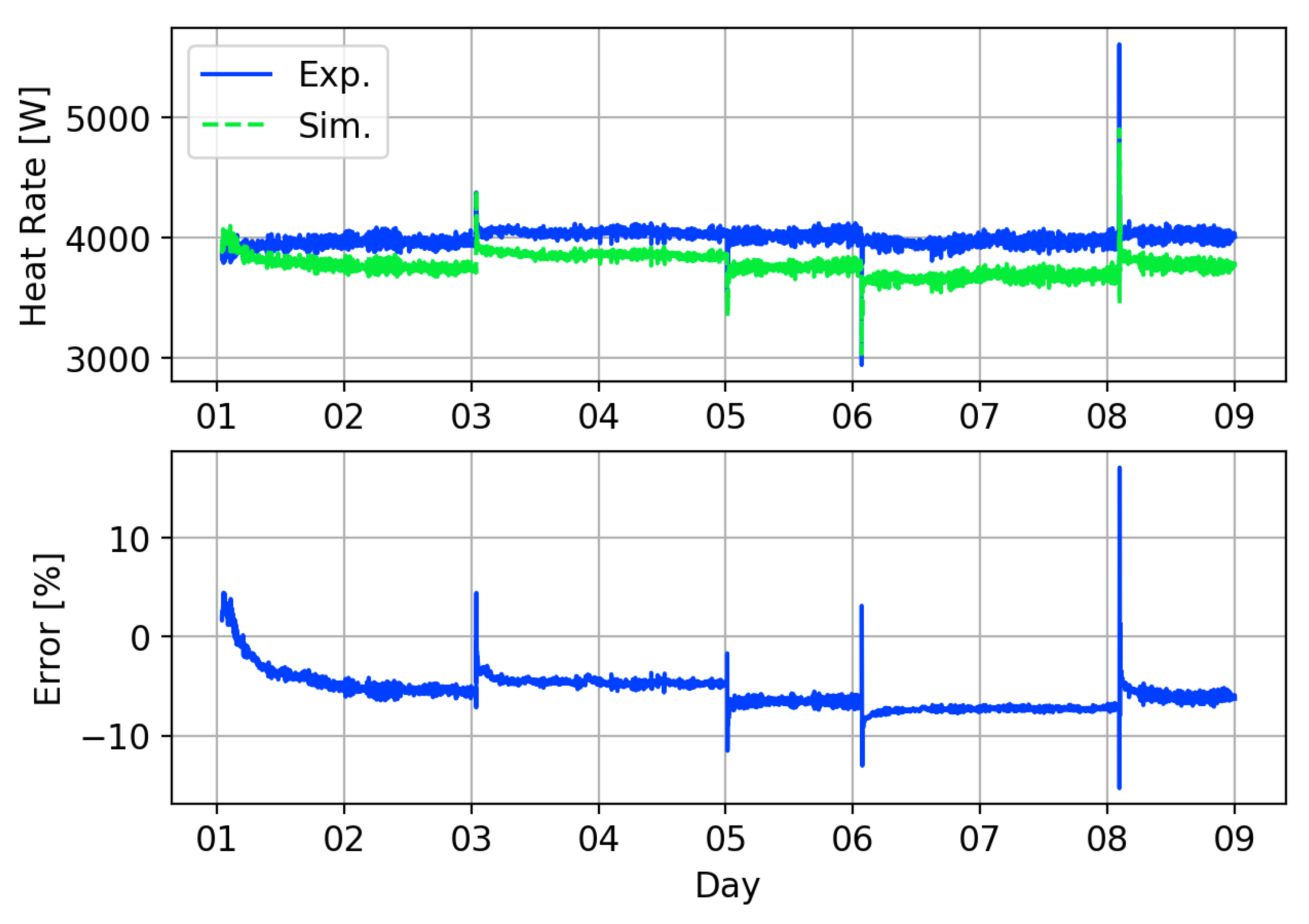
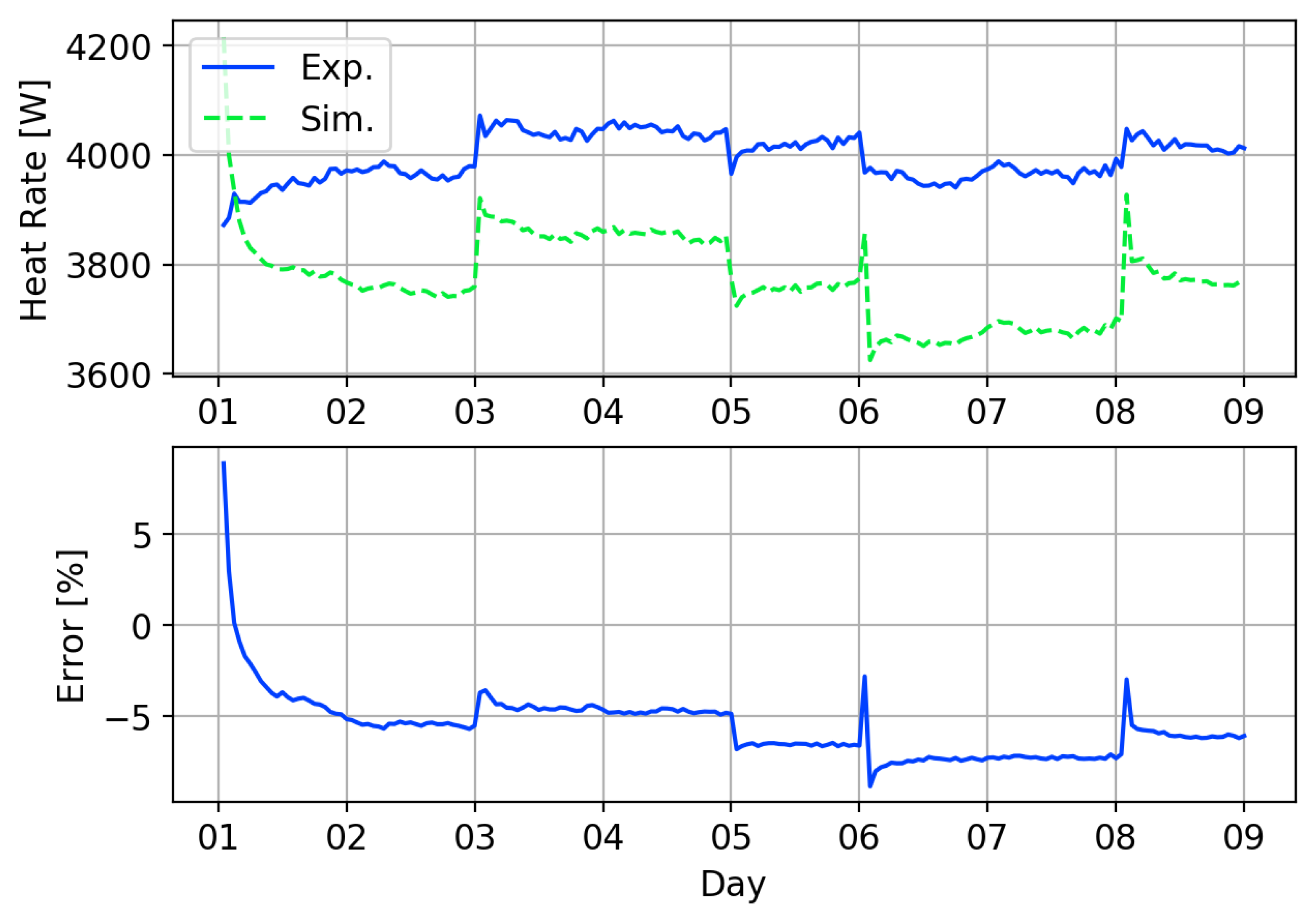
4.1. High-Flow MFRTRT

Figure 11 shows the temperature comparison for the first two hours of the high-flow MFRTRT. The simulation was run using a 60-s timestep. As occurred during the comparison of the dynamic borehole model, some transit delay errors are present during the first five minutes of the simulation, which result in some error in the temperature predicted. However, once the first few transit periods have passed, the model and experimental data agree quite well.
Figure 12 shows the temperature comparison for the first flow rate change using a 60-s timestep. During this period, the flow rate is changed from approximately 0.3 k g / s up to 0.45 k g / s , which results in a smaller temperature difference between the inlet and outlet of the GHE. The figure shows good a dynamic response compared to the experiment during this step change in flow, and the absolute outlet temperature error remains under 0.2 C .
Figure 13 and Figure 14 show the full high-flow MFRTRT data compared using the enhanced response factor model using 60-s and 1-h timesteps, respectively. Figure 13, as in previous plots, shows higher errors at times when the flow rate changes, but level off after that. Again, these errors are attributed to the errors in the transit time predicted using the dynamic borehole model. The overall temperature difference is generally under predicted by less than 0.5 C .
For the simulation using a 1-h timestep shown in Figure 14, these transit time errors are not present because a 1-h timestep is 10– 30 × the GHE transit time. The overall trend of the exiting fluid temperature error is consistent with the 60-s timestep simulation data.
Figure 15 and Figure 16 show the heat transfer error from the experimental data and the simulation, for a 60-s and 1-h timestep, respectively. In both cases, the heat transfer error is within 10%, except during flow changes, and near 5–6% for the test duration. Note that the experimental uncertainty in the heat transfer measurements is not shown here but is discussed in Beier et al. [70]. For the high-flow test, the heat transfer error is generally around ±3–7%, depending on flow rate. Additionally, note that the soil and grout parameters are estimated values, and that changes in these values can easily affect the results enough to affect the error predicted. Further optimization of the soil and grout parameter values could result in reductions to the overall error.

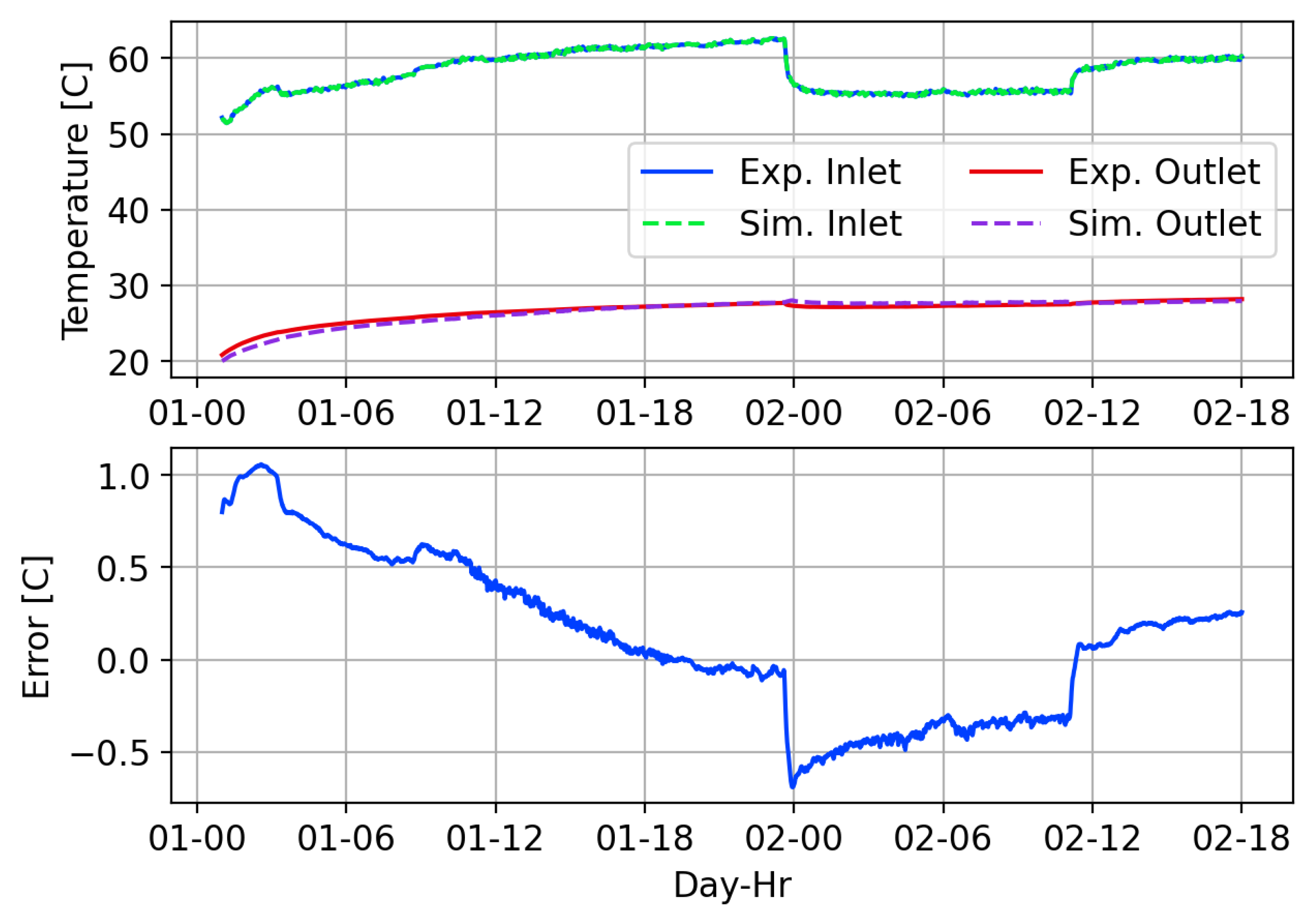
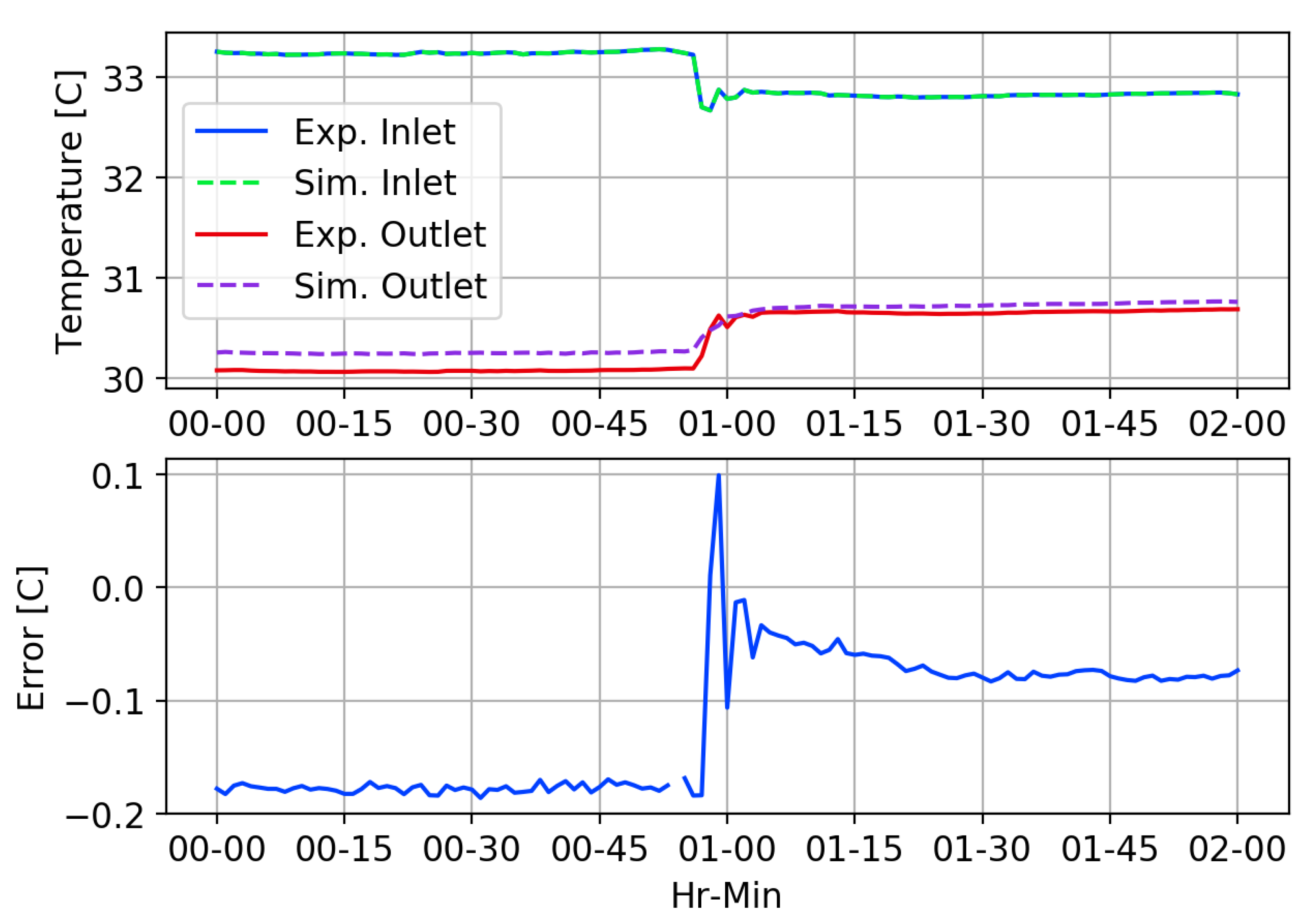
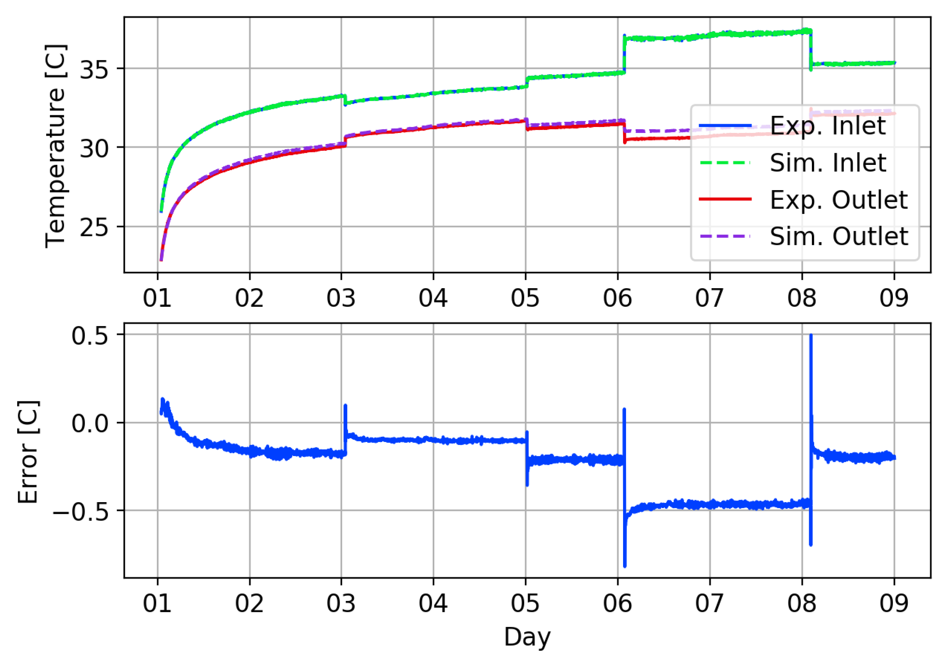
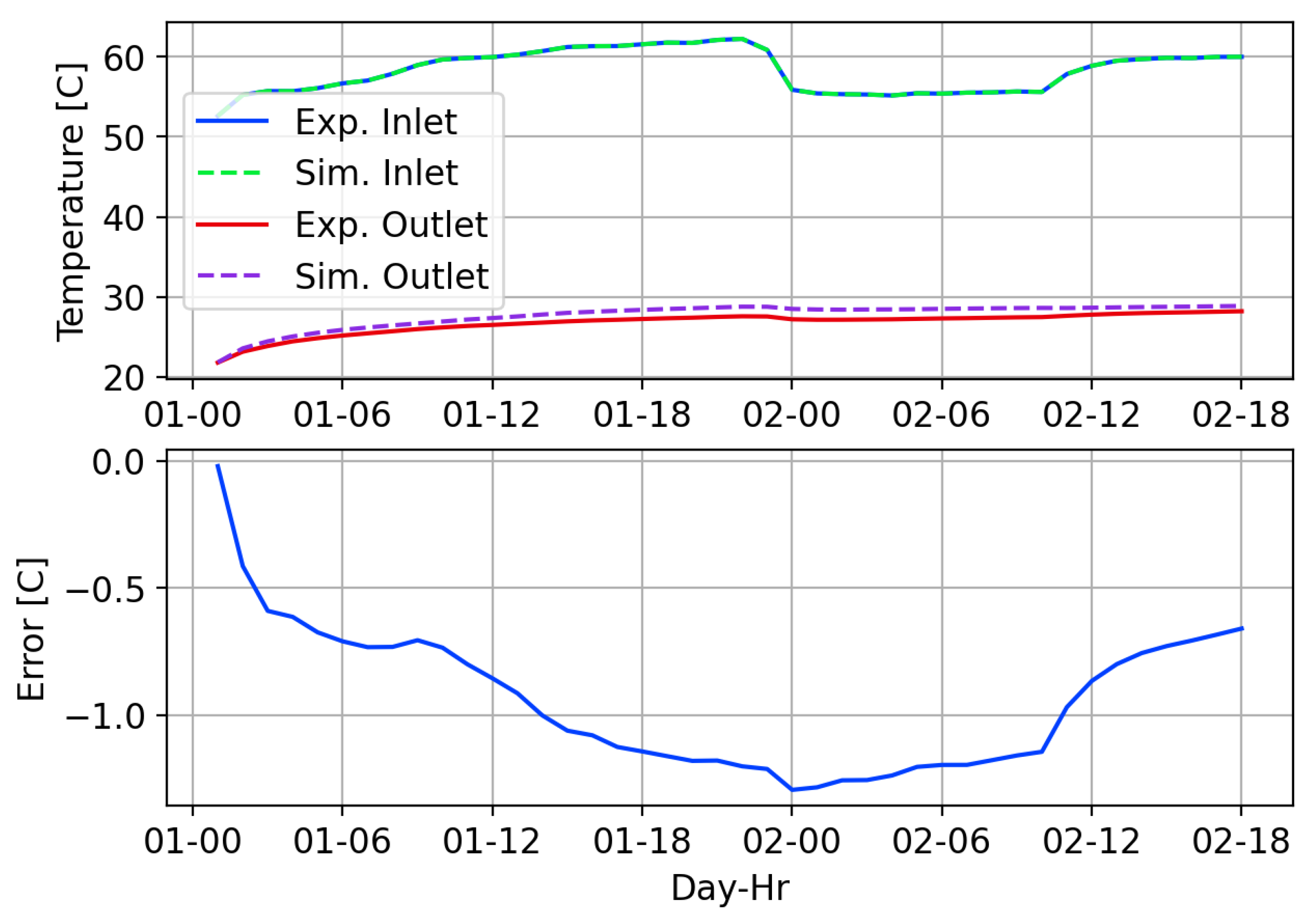
4.2. Low-Flow MFRTRT

Figure 17 shows the model compared to 68 h of data from the low-flow MFRTRT. The absolute exiting fluid temperature error is higher than the high-flow test, as the temperature difference is under predicted by about 1 C . As with the high-flow test, a similar error can be seen from in Figure 8 from the direct simulation using the dynamic borehole model. Again, this suggests that errors in the enhanced response factor method can be addressed by improving the accuracy of the dynamic borehole model used to generate the ExFT g-functions.
Figure 18 shows the heat transfer results for the low-flow test compared to the simulation. As before, the experimental heat transfer rate errors are not plotted, but, for this particular flow rate, they are around ±3%. Variations in soil properties will also affect the results, and in practice the inlet temperatures and heat transfer rates will be adjusted naturally during an overall system simulation.

5. Conclusions

This work describes an enhanced response factor model for use in whole-building energy simulation environments. This model combines long-timestep and short-timestep g-functions that give responses at the borehole wall, with the exiting fluid temperature g-functions proposed by Pasquier et al. [32]. Using the new model, our research has shown that accurate dynamic behavior can be simulated for GHE using response factor calculations. The results are shown to be accurate for timesteps that are shorter than the GHE transit time, as well as for long timesteps.
A simplified dynamic borehole model was also developed, which is used to generate exiting fluid temperature g-functions. A Pareto front analysis was performed to determine the optimized model parameters for speed and accuracy. Computation time for the exiting fluid temperature g-functions was shown to be computed in less than 8 s on a desktop PC while keeping the root mean squared error below 3 C . Inaccuracies in the enhanced response factor model were shown to be directly related to inaccuracies in the simplified dynamic borehole model, though the methods generally compare well against experimental MFRTRT measurements.
The new method requires computation of long-timestep, short-timestep, and exiting fluid temperature g-function values; however, the methods utilized here are efficient and are acceptable for WBES applications. Given some intelligent programming, the g-functions would only need to be computed one time for each unique GHE configuration. If the GHE configuration is not changed between simulations, the g-function values could be saved and reused during subsequent simulations.
Although this work has shown that the model is sufficiently fast and acceptably accurate, further research in these areas might improve accuracy, computational speed, and applicability to different ground heat exchanger types:
  • The pipe model currently used does not account for laminar flow; therefore, the pipe model should be enhanced to accurately account for these conditions.
  • Any dynamic borehole model could be used to generate ExFT g-functions; therefore, a study should be performed to assess this model along with other existing models for accuracy and performance.
  • The methods described here could also be used to model double U-tube or coaxial ground heat exchangers. Dynamic borehole models for these configurations would be needed in order to calculate the ExFT g-functions.

Author Contributions

Both authors contributed to this work as follows: Conceptualization, M.S.M. and J.D.S.; methodology, M.S.M. and J.D.S.; software, M.S.M; validation, M.S.M. and J.D.S.; formal analysis, M.S.M. and J.D.S.; investigation, M.S.M. and J.D.S.; resources, M.S.M. and J.D.S.; data curation, M.S.M. and J.D.S.; writing—original draft preparation, M.S.M. and J.D.S.; writing—review and editing, M.S.M. and J.D.S.; visualization, M.S.M. and J.D.S.; supervision, J.D.S.; project administration, M.S.M.; funding acquisition, M.S.M. All authors have read and agreed to the published version of the manuscript.

Funding

This work was authored in part by the National Renewable Energy Laboratory, operated by Alliance for Sustainable Energy, LLC, for the U.S. Department of Energy (DOE) under Contract No. DE-AC36-08GO28308. Funding was provided by the U.S. Department of Energy Office of Energy Efficiency and Renewable Energy Building Technologies Office. The views expressed in the article do not necessarily represent the views of the DOE or the U.S. Government. The U.S. Government retains and the publisher, by accepting the article for publication, acknowledges that the U.S. Government retains a nonexclusive, paid-up, irrevocable, worldwide license to publish or reproduce the published form of this work, or allow others to do so, for U.S. Government purposes. The work performed was partially supported under the National Renewable Energy Laboratory Task Order Agreement KAGN-4-42503-00.

Acknowledgments

The authors gratefully acknowledge Oklahoma State University and The National Renewable Energy Laboratory for supporting this work.

Conflicts of Interest

The authors declare no conflict of interest.

Abbreviations

The following abbreviations are used in this manuscript:
ExFTexiting fluid temperature
FLSfinite line source
GHEground heat exchanger
GSHPground-source heat pump
ICSinfinite cylinder source
ILSinfinite line source
MFRTRTmulti-flowrate thermal response test
TRCthermal resistance-capacitance
TRTthermal response test
WBESwhole-building energy simulation

References

  1. Crawley, D.B.; Lawrie, L.K.; Winkelmann, F.C.; Buhl, W.F.; Huang, Y.J.; Pedersen, C.O.; Strand, R.K.; Liesen, R.J.; Fisher, D.E.; Witte, M.J.; et al. EnergyPlus: Creating a new-generation building energy simulation program. Energy Build. 2001, 33, 319–331. [Google Scholar] [CrossRef]
  2. Klein, S.A.; Beckman, W.A.; Mitchell, J.W.; Duffie, J.A.; Duffie, N.A.; Freeman, T.; Mitchell, J.C.; Braun, J.E.; Evans, B.L.; Kummer, J.P.; et al. TRNSYS Manual: A Transient Simulation Program; Solar Engineering Laboratory; University of Wisconsin-Madison: Madison, WI, USA, 2016. [Google Scholar]
  3. Li, M.; Zhu, K.; Fang, Z. Analytical methods for thermal analysis of vertical ground heat exchangers. In Advances in Ground-Source Heat Pump Systems; Woodhead Publishing: Duxford, UK, 2016; pp. 157–185. [Google Scholar]
  4. Spitler, J.D.; Bernier, M.A. Vertical borehole ground heat exchanger design methods. In Advances in Ground-Source Heat Pump Systems; Woodhead Publishing: Duxford, UK, 2016; pp. 29–61. [Google Scholar]
  5. Thomson, W. Compendium of the Fourier Mathematics for the Conduction of Heat in Solids, and the Mathematically Allied Physical Subjects of Diffusion of Fluids, and Transmission of Electrical Signals Through Submarine Cables. In Article 72. Mathematical and Physical Papers; University Press: Cambridge, UK, 1884; pp. 41–60. [Google Scholar]
  6. Spitler, J.D.; Gehlin, S.E.A. Thermal response testing for ground source heat pump systems—An historical review. Renew. Sustain. Energy Rev. 2015, 50, 1125–1137. [Google Scholar] [CrossRef]
  7. Carslaw, H.S.; Jaeger, J.C. Conduction of Heat in Solids, 2nd ed.; Clarendon Press: London, UK, 1959. [Google Scholar]
  8. Hellström, G. Ground Heat Storage: Thermal Analysis of Duct Storage Systems. Ph.D. Thesis, University of Lund, Lund, Sweden, 1991. [Google Scholar]
  9. Mogensen, P. Fluid to duct wall heat transfer in dust system heat storages. In International Conference on Subsurface Heat Storage in Theory and Practice; Swedish Council for Building Research: Stockholm, Sweden, 1983. [Google Scholar]
  10. Bernier, M.A. Ground-coupled heat pump system simulation. ASHRAE Trans. 2001, 107, 605–616. [Google Scholar]
  11. Ingersoll, L.R.; Zobel, O.J.; Ingersoll, A.C. Heat Conduction: With Engineering and Geological Applications, 2nd ed.; McGraw-Hill: New York, NY, USA, 1954. [Google Scholar]
  12. Diao, N.R.; Li, Q.Y.; Fang, Z. Heat transfer in ground heat exchangers with ground water advection. Int. J. Therm. Sci. 2004, 43, 1203–1211. [Google Scholar] [CrossRef]
  13. Man, Y.; Yang, H.; Diao, N.R.; Liu, J.; Fang, Z.H. A new model and analytical solutions for borehole and pile ground heat exchangers. Int. J. Heat Mass Transf. 2010, 53, 2593–2601. [Google Scholar] [CrossRef]
  14. Li, M.; Lai, L.C.K. Heat-source solutions to heat conduction in anisotropic media with applications to pile and borehole ground heat exchangers. Appl. Energy 2012, 96, 451–458. [Google Scholar] [CrossRef]
  15. Marcotte, D.; Pasquier, P. The effect of borehole inclination on fluid and ground temperature for GLHE systems. Geothermics 2009, 38, 392–398. [Google Scholar] [CrossRef]
  16. Lamarche, L.; Beauchamp, B. A new contribution to the finite line-source model for geothermal boreholes. Energy Build. 2007, 39, 188–198. [Google Scholar] [CrossRef]
  17. Javed, S.; Claesson, J. New analytical and numerical solutions for the short-term analysis of vertical ground heat exchangers. ASHRAE Trans. 2011, 117, 3–12. [Google Scholar]
  18. Grundmann, R.M. Improved Design Methods for Ground Heat Exchangers. Master’s Thesis, Oklahoma State University, Stillwater, OK, USA, 2016. [Google Scholar]
  19. Spitler, J.D. GLHEPro—A design tool for commercial building ground loop heat exchangers. In Proceedings of the 4th International Heat Pump in Cold Climates Conference, Alymer, QC, Canada, 17–18 August 2000. [Google Scholar]
  20. Duhamel, M.J.M.C. Sur les equations générales de la propagation de la chaleur dan les corps solides dont la conductiblité n’est pas la même dan tous les sens. J. L’Ecole Polytech. 1828, 21, 356–399. [Google Scholar]
  21. Özişik, M.N. Boundary Value Problems of Heat Conduction; Dover Publications: New York, NY, USA, 2002. [Google Scholar]
  22. Claesson, J.; Dunand, A. Heat Extraction from the Ground by Horizontal Pipes—A Mathematical Analysis; Technical Report; Swedish Council for Building Research: Stockholm, Sweden, 1983. [Google Scholar]
  23. Eskilson, P. Thermal Analysis of Heat Extraction Boreholes. Ph.D. Thesis, University of Lund, Lund, Sweden, 1987. [Google Scholar]
  24. Claesson, J.; Eskilson, P. Conductive heat extraction to a deep borehole—Thermal analysis and dimensioning rules. Energy 1988, 13, 509–527. [Google Scholar] [CrossRef]
  25. Eskilson, P.; Claesson, J. Simulation model for thermally interacting heat extraction boreholes. Numer. Heat Transf. 1988, 13, 149–165. [Google Scholar] [CrossRef]
  26. Mitchell, M.S.; Spitler, J.D. Characterization, testing, and optimization of load aggregation methods for ground heat exchanger response-factor models. Sci. Technol. Built Environ. 2019, 8, 1036–1051. [Google Scholar] [CrossRef]
  27. Brussieux, Y.; Bernier, M. Universal short time g*-functions: Generation and application. Sci. Technol. Built Environ. 2019, 8, 993–1006. [Google Scholar] [CrossRef]
  28. Loveridge, F.; Powrie, W. Temperature response functions (G-functions) for single pile heat exchangers. Energy 2013, 57, 554–564. [Google Scholar] [CrossRef]
  29. Alberdi-Pagola, M. Design and Performance of Energy Pile Foundations. Ph.D. Thesis, Aalborg University, Aalborg, Denmark, 2018. [Google Scholar]
  30. Alberdi-Pagola, M.; Jensen, R.L.; Poulsen, S.; Erbs, S. Method to Obtain G-Functions for Multiple Precast Quadratic Pile Heat Exchangers; Technical Report 243; Aalborg University: Aalborg Øst, Denmark, 2018. [Google Scholar]
  31. Dusseault, B.; Pasquier, P. Efficient g-function approximation with artificial neural networks for a varying number of boreholes on a regular or irregular layout. Sci. Technol. Built Environ. 2019, 8, 1023–1035. [Google Scholar] [CrossRef]
  32. Pasquier, P.; Zarrella, A.; Labib, R. Application of artificial neural networks to near-instant construction of short-term g-functions. Appl. Therm. Eng. 2018, 143, 910–921. [Google Scholar] [CrossRef]
  33. Pasquier, P.; Marcotte, D. Short-term simulation of ground heat exchanger with an improved TRCM. Renew. Energy 2012, 46, 92–99. [Google Scholar] [CrossRef]
  34. Pasquier, P.; Marcotte, D. Joint use of quasi-3D response model and spectral method to simulate borehole heat exchanger. Geothermics 2014, 51, 281–299. [Google Scholar] [CrossRef]
  35. Cimmino, M.; Bernier, M. A semi-analytical method to generate g-functions for geothermal bore fields. Int. J. Heat Mass Transf. 2014, 70, 641–650. [Google Scholar] [CrossRef]
  36. Malayappan, V.; Spitler, J.D. Limitation of using uniform heat flux assumptions in sizing vertical borehole heat exchanger fields. In Proceedings of the CLIMA 2013, Prague, Czech Republic, 16–19 June 2013. [Google Scholar]
  37. Marcotte, D.; Pasquier, P. Unit-response function for ground heat exchanger with parallel, series or mixed borehole arrangement. Renew. Energy 2014, 68, 14–24. [Google Scholar] [CrossRef]
  38. Claesson, J.; Javed, S. An analytical method to compute borehole fluid temperatures for timescales from minutes to decades. ASHRAE Trans. 2011, 117, 279–288. [Google Scholar]
  39. Cimmino, M. Fast calculation of the g-functions of geothermal borehole fields using similarities in the evaluation of the finite line source solution. J. Build. Perform. Simul. 2018, 11, 655–668. [Google Scholar] [CrossRef] [Green Version]
  40. Cimmino, M. g-Functions for bore fields with mixed parallel and series connections considering axial fluid temperature variations. In Proceedings of the IGSHPA Research Conference Proceedings, IGSHPA, Stockholm, Sweden, 18–19 September 2018; pp. 262–271. [Google Scholar]
  41. Cimmino, M. Semi-analytical method for g-function calculation of bore fields with series- and parallel-connected boreholes. Sci. Technol. Built Environ. 2019, 25, 1007–1022. [Google Scholar] [CrossRef]
  42. Cimmino, M. pygfunction: An open-source toolbox for the evaluation of thermal response factors for geothermal borehole fields. In Proceedings of the eSim 2018, the 10th Conference of IBPSA-Canada, International Building Performance Simulation Association, Montréal, QC, Canada, 9 March 2018; pp. 492–501. [Google Scholar] [CrossRef]
  43. De Carli, M.; Tonon, M.; Zarrella, A.; Zecchin, R. A computational capacity resistance model (CaRM) for vertical ground-coupled heat exchangers. Renew. Energy 2010, 35, 1537–1550. [Google Scholar] [CrossRef]
  44. Zarrella, A.; Scarpa, M.; De Carli, M. Short time step analysis of vertical ground-coupled heat exchangers: The approach of CaRM. Renew. Energy 2011, 36, 2357–2367. [Google Scholar] [CrossRef]
  45. Bauer, D.; Heidemann, W.; Müller-Steinhagen, H.; Diersch, H.J.G. Thermal resistance and capacity models for borehole heat exchangers. Int. J. Energy Res. 2011, 35, 312–320. [Google Scholar] [CrossRef]
  46. Ruiz-Calvo, F.; De Rosa, M.; Acuña, J.; Corberán, J.M.; Montagud, C. Experimental validation of a short-term borehole-to-ground (B2G) dynamic model. Appl. Energy 2015, 140, 210–223. [Google Scholar] [CrossRef] [Green Version]
  47. Cazorla-Marín, A.; Montagud, C.; Montero, Á.; Martos, J.; Corberán, J.M. Influence of different ground thermal properties in a borehole heat exchanger’s performance using the B2G dynamic model. In Proceedings of the IGSHPA Research Conference, IGSHPA, Denver, CO, USA, 14–16 March 2017; pp. 192–200. [Google Scholar]
  48. Ruiz-Calvo, F.; De Rosa, M.; Monzó, P.; Montagud, C.; Corberán, J.M. Coupling short-term (B2G model) and long-term (g-function) models for ground source heat exchanger simulation in TRNSYS. Application in a real installation. Appl. Therm. Eng. 2016, 102, 720–732. [Google Scholar] [CrossRef]
  49. Al-Khoury, R. Spectral framework for geothermal borehole heat exchangers. Int. J. Numer. Methods Heat Fluid Flow 2010, 20, 773–793. [Google Scholar] [CrossRef]
  50. Shao, H.; Hein, P.; Sachse, A.; Kolditz, O. Geoenergy Modeling II: Shallow Geothermal Systems; Springer: Cham, Switzerland, 2016. [Google Scholar]
  51. Al-Khoury, R.; Bonnier, P.G.; Brinkgreve, R.B.J. Efficient finite element formulation for geothermal heating systems–Part I: Steady state. Int. J. Numer. Methods Eng. 2005, 63, 988–1013. [Google Scholar] [CrossRef]
  52. Al-Khoury, R.; Bonnier, P.G. Efficient finite element formulation for geothermal heating systems–Part II: Transient. Int. J. Numer. Methods Eng. 2006, 67, 725–745. [Google Scholar] [CrossRef]
  53. He, M.; Rees, S.; Shao, L. Simulation of a domestic ground source heat pump system using a three-dimensional numerical borehole heat exchanger model. J. Build. Perform. Simul. 2011, 4, 141–155. [Google Scholar] [CrossRef]
  54. Nabi, M.; Al-Khoury, R. An efficient finite volume model for shallow geothermal systems–Part I: Model formulation. Comput. Geosci. 2012, 49, 290–296. [Google Scholar] [CrossRef]
  55. Nabi, M.; Al-Khoury, R. An efficient finite volume model for shallow geothermal systems–Part II: Verification, validation and grid convergence. Comput. Geosci. 2012, 49, 297–307. [Google Scholar] [CrossRef]
  56. Fisher, D.E.; Rees, S.J.; Padhmanabhan, S.K.; Murugappan, A. Implementation and validation of ground-source heat pump system models in an integrated building and system simulation environment. HVAC&R Res. 2006, 12, 693–710. [Google Scholar] [CrossRef]
  57. Yavuzturk, C.; Spitler, J.D. A short time step response factor model for vertical ground loop heat exchangers. ASHRAE Trans. 1999, 105, 475–485. [Google Scholar]
  58. Xu, X.; Spitler, J.D. Modeling of vertical ground loop heat exchangers with variable convective resistance and thermal mass of the fluid. In Proceedings of the 10th International Conference on Thermal Energy Storage-EcoStock, Pomona, NJ, USA, 31 May–2 June 2006. [Google Scholar]
  59. Mitchell, M.S. An Enhanced Vertical Ground Heat Exchanger Model for Whole Building Energy Simulation. Ph.D. Thesis, Oklahoma State University, Stillwater, OK, USA, 2019. [Google Scholar]
  60. Loveridge, F. The Thermal Performance of Foundation Piles Used as Heat Exchangers in Ground Energy Systems. Ph.D. Thesis, University of Southampton, Southampton, UK, 2012. [Google Scholar]
  61. Bennet, J.; Claesson, J.; Helström, G. Multipole Method to Compute the Conductive Heat Flow to and between Pipes in a Composite Cylinder; Technical Report; University of Lund, Department of Building and Mathematical Physics: Lund, Sweden, 1987. [Google Scholar]
  62. Claesson, J. Multipole Method to Calculate Borehole Thermal Resistances: Mathematical Report; Technical Report 2012-06-20; Chalmers Technical University: Gothenburg, Sweden, 2011. [Google Scholar]
  63. Claesson, J.; Hellström, G. Multipole method to calculate borehole thermal resistances in a borehole heat exchanger. HVAC&R Res. 2011, 17, 895–911. [Google Scholar] [CrossRef]
  64. Javed, S.; Spitler, J.D. Accuracy of borehole thermal resistance calculation methods for grouted single u-tube ground heat exchangers. Appl. Energy 2017, 187, 790–806. [Google Scholar] [CrossRef]
  65. Javed, S.; Spitler, J.D. Chapter Calculation of Borehole Thermal Resistance. In Advances in Ground-Source Heat Pump Systems; Woodhead Publishing: Duxford, UK, 2016; pp. 63–95. [Google Scholar]
  66. Moin, P. Fundamentals of Engineering Numerical Analysis; Cambridge University Press: New York, NY, USA, 2010. [Google Scholar]
  67. Bischoff, K.B.; Levenspiel, O. Fluid dispersion—generalization and comparison of mathematical models—II comparison of models. Chem. Eng. Sci. 1962, 17, 257–264. [Google Scholar] [CrossRef]
  68. Skoglund, T.; Dejmek, P. A dynamic object-oriented model for efficient simulation of fluid dispersion in turbulent flow with varying fluid properties. Chem. Eng. Sci. 2007, 62, 2168–2178. [Google Scholar] [CrossRef] [Green Version]
  69. Rees, S.J. An extended two-dimensional borehole heat exchanger model for simulation of short and medium timescale thermal response. Renew. Energy 2015, 83, 518–526. [Google Scholar] [CrossRef] [Green Version]
  70. Beier, R.A.; Mitchell, M.S.; Spitler, J.D.; Javed, S. Validation of borehole heat exchanger models against multi-flow rate thermal response tests. Geothermics 2018, 71, 55–68. [Google Scholar] [CrossRef]
  71. Woodruff, M.J.; Herman, J. Pareto. 2018. Available online: https://github.com/matthewjwoodruff/pareto.py (accessed on 1 October 2018).
  72. Deb, K.; Pratap, A.; Agarwal, S.; Meyarivan, T. A fast and elitist multiobjective genetic algorithm: NSGA-II. IEEE Trans. Evol. Comput. 2002, 6, 182–197. [Google Scholar] [CrossRef] [Green Version]
  73. Bell, I.H.; Wronski, J.; Quoilin, S.; Lemort, V. Pure and pseudo-pure fluid thermophysical property evaluation and the open-source thermophysical property library CoolProp. Ind. Eng. Chem. Res. 2014, 53, 2498–2508. [Google Scholar] [CrossRef] [PubMed] [Green Version]
  74. Patankar, S.V. Computation of Conduction and Duct Flow Heat Transfer; Innovative Research, Inc.: Maple Grove, MN, USA, 1991. [Google Scholar]
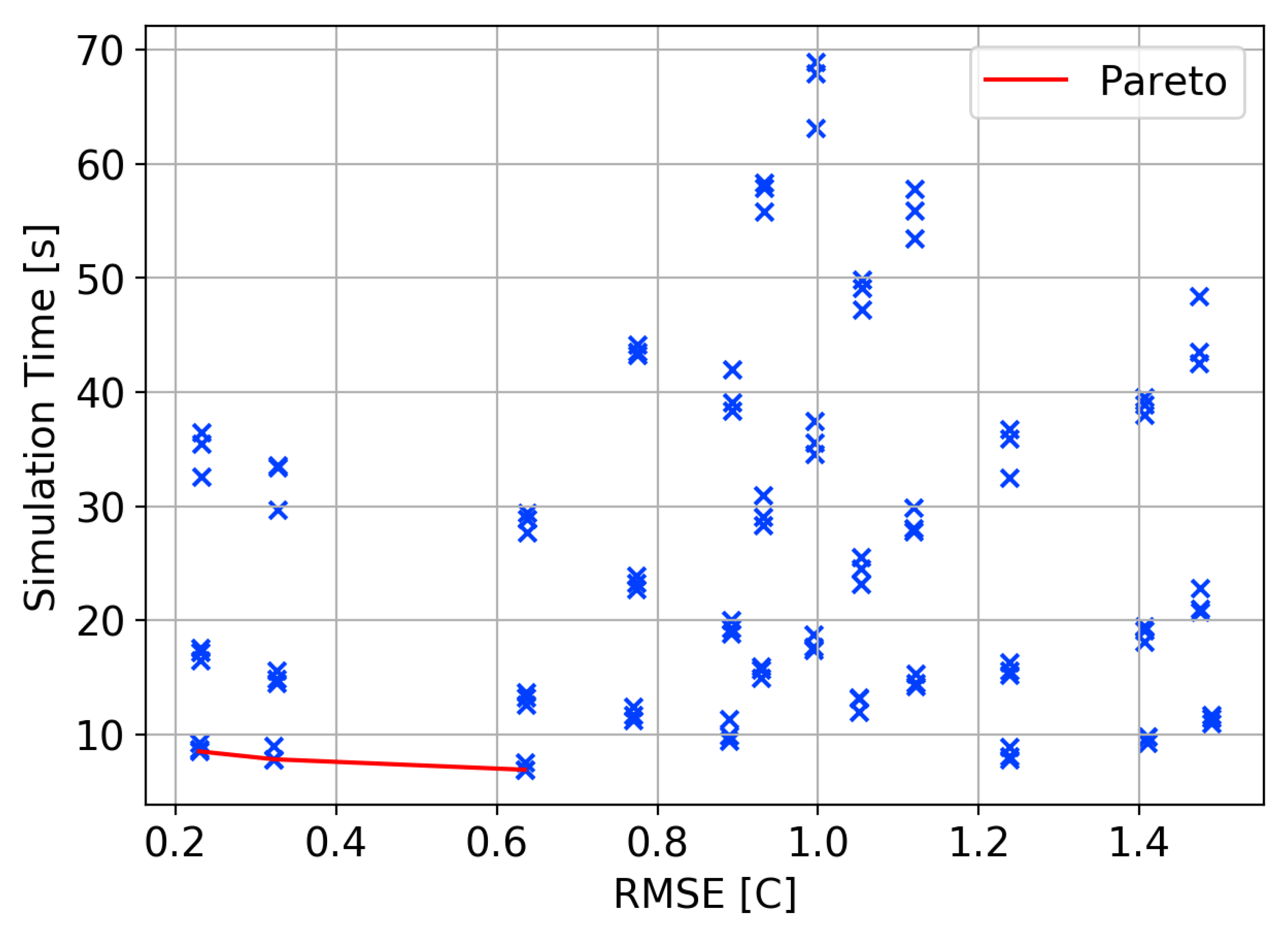
Figure 1. Example g-functions for a 3 × 2 rectangular GHE array.
Energies 13 04058 g001
Figure 2. RC-network geometrical representation.
Energies 13 04058 g002
Figure 3. Single U-tube borehole.
Energies 13 04058 g003
Figure 4. Dynamic model borehole schematic.
Energies 13 04058 g004
Figure 5. Simple TRC model.
Energies 13 04058 g005
Figure 6. Pareto values for variations in dynamic borehole model input parameters (note: RMSE = root mean squared error).
Energies 13 04058 g006
Figure 7. Dynamic borehole model compared to high-flow MFRTRT.
Energies 13 04058 g007
Figure 8. Dynamic borehole model compared to 2 days of low-flow MFRTRT.
Energies 13 04058 g008
Figure 9. g b vs. ln ( t / t s ) .
Energies 13 04058 g009
Figure 10. g vs. ln ( t / t s ) .
Energies 13 04058 g010
Figure 11. Enhanced model results for high-flow MFRTRT. First 2 h. 60-s timestep.
Energies 13 04058 g011
Figure 12. Enhanced model results for high-flow MFRTRT. First flow rate change. 60-s timestep.
Energies 13 04058 g012
Figure 13. Enhanced model results for high-flow MFRTRT. Full data set. 60-s timestep.
Energies 13 04058 g013
Figure 14. Enhanced model results for high-flow MFRTRT. Full data set. 1-hr timestep.
Energies 13 04058 g014
Figure 15. Enhanced model heat transfer results for high-flow MFRTRT. Full data set. 60-s timestep.
Energies 13 04058 g015
Figure 16. Enhanced model heat transfer results for high-flow MFRTRT. Full data set. 1-hr timestep.
Energies 13 04058 g016
Figure 17. Enhanced model temperature results for low-flow MFRTRT. Full data set. 1-hr timestep.
Energies 13 04058 g017
Figure 18. Enhanced model heat transfer results for low-flow MFRTRT. Full data set. 1-hr timestep.
Energies 13 04058 g018
Table 1. Dynamic borehole model Pareto data (note: MBE = mean bias error).
N it N seg Δ t f g RMSE [C]MBE [C]Time [s]
31600.750.229−0.0738.5
21600.50.322−0.1697.8
11600.50.634−0.4486.9
Table 2. Data from g b calculations taken at t = 24   h .
m ˙ f Re ln ( t / t s ) g b T out T b q f R b T out T b q f · R b
kg/s---°C°C(W/m)°C/(W/m)°C°C
0.021400−8.80.6718.8017.349.9890.2161.452.16
0.031967−8.80.7118.8917.359.9910.2171.552.16
0.042534−8.80.7418.9217.359.9930.2111.572.11
0.053079−8.80.7518.6217.359.9940.1691.271.69
0.15894−8.80.8118.6217.369.9960.1541.261.54
0.317,209−8.80.9118.7317.369.9960.1511.371.51
0.528,535−8.80.9418.7617.369.9940.1501.401.50

