Abstract
This paper focuses on the interdependent relationship of power generation, transportation and CO emissions to evaluate the impact of electric vehicle deployment on power generation and CO emissions. The value of this evaluation is in the employment of a large-scale, bottom-up, national energy modeling system that encompasses the complex relationships of producing, transforming, transmitting and supplying energy to meet the useful demand characteristics with great technological detail. One of such models employed in this analysis is the BUEMS model. The BUEMS model provides evidence of win-win policy options that lead to profitable decarbonization using Turkey’s data in BUEMS. Specifically, the result shows that a ban on diesel fueled vehicles reduces lifetime emissions as well as lifetime costs. Furthermore, model results highlight the cost-effective emission reduction potential of e-buses in urban transportation. More insights from the results indicate that the marginal cost of emission reduction through e-bus transportation is much lower than that through other policy measures such as carbon taxation in transport. This paper highlights the crucial role the electricity sector plays in the sustainability of e-mobility and the value of related policy prescriptions.
1. Introduction
Globally, the energy sector is the main contributor to CO emissions followed by transportation. For example, the International Energy Agency [1] indicates that global CO emissions from fuel combustion in 2017 were 32.8 Gt, growing from 32.3 Gt in 2016. The report highlights that electricity/heat generation and transport account for two-thirds of total CO emissions and were equally responsible for almost the entire global growth in emissions since 2010. Emissions from the transport sector account for approximately a quarter of energy-related CO emissions worldwide, while road vehicles account for nearly three-quarters of transport CO emissions. In the Fifth Assessment Report (AR5), the Intergovernmental Panel on Climate Change (IPCC) highlights that emissions from the transport sector have been increasing at a faster rate than any other energy end-use sector [2,3]. Emissions from transportation are on the rise, essentially due to greater overall volume of travel that outweighs improvements in the energy efficiency of vehicles.
Advancements in e-mobility technology with significant reductions in battery prices and increase in efficiencies expedite the diffusion prospects of plug-in electric vehicles. Similar advancements in hydrogen vehicles and vehicle to grid (V2G) technology brighten the future of e-mobility as a sustainable solution for the transport sector with zero emissions on the road. However, a systemic analysis is needed for understanding the overall implications on energy demand and CO emissions of electrification in transport. In particular, it becomes important how the additional electricity required is supplied. Switching from internal combustion vehicles to electric vehicles may not be sustainable if the increased electricity demand is generated in coal-fired power plants as the net effect on CO emissions would be a rise. While it is indeed true that plug-in electric vehicles do not directly emit greenhouse gas emissions, there are indirect emissions due to the electricity generated to recharge the vehicle batteries. The optimal configuration of the sources of electricity often result from the dynamics of the competition [4], state of technological progress [5] or responses to uncertainties in regulations [6] or reliability [7] of the technology portfolio. Some best practices for future grid emissions indicate that plug-in electric vehicles can reduce transportation emissions [8].
The composition of CO emission sources in Turkey resembles the global picture. The energy sector is responsible for 41% of total CO emissions while the transport sector accounts for 23% according to the latest National Inventory Submission [9]. Emissions from oil products, mainly used in the transport sector, account for 27%. Road transportation is responsible for 93% of CO emissions from the transport sector, containing 90% of all passenger transport and 89% of all freight transport. Considering newly registered vehicles, the share of diesel cars has strongly increased to 63% over the past decade. Road transportation contains 90% of all passenger transport and 89% of all freight; it dominates Turkey’s transport sector and is responsible for 93% of CO emissions from the transport sector. While rail transportation accounts for 4.4% of freight and 1% of passenger transport, maritime supplies 6% of freight transport. Considering newly registered vehicles in 2017, the share of diesel cars has strongly increased by 63% over the past decade.
Based upon this interdependent relationship of power generation, transportation and CO emissions, this study evaluates the impact of electric vehicle deployment on power generation and CO emissions in Turkey using the Bottom-Up Energy Modeling System (BUEMS), which is designed as a large-scale linear optimization model. The objective of this paper is to answer an integrated set of questions related to how the transportation sector, despite the advances in vehicular fuel efficiencies and through plug-in electric vehicles, influences overall energy demand, cost and CO emissions. This paper sheds light on the influence of electrifying transportation on the carbon footprints of the increased demand for electricity. The paper tests the central hypothesis that a transition to electric vehicles increases carbon emissions the higher the dependence of the aggregate electricity demand on fossil technologies. A contribution of the paper highlights the unintended and indirect consequences of increased transport electrification without considerations for grid decarbonization. While the extant literature on the topic has argued for reduced emissions, this paper deviates by underscoring that emissions may be higher depending on the carbon intensity of power generation and the underlying scenarios. More significantly, the implication for policy shows that the marginal cost of emission reduction through e-buses is much lower than through other policy measures like carbon taxation.
The rest of this paper proceeds with the description of the energy modeling applications in transportation. Section 2 presents an abridged summary of related literature within the context of energy modeling applications in transportation. Section 3 is focused on the underlying mathematical formulations that drive the BUEMS modeling structure. Section 4 presents an elaborate description of the reference energy model. Section 5 proceeds with the calibration of the model while Section 6 presents the results of the analysis. To understand the influence of specific differences in model parameters, Section 7 conducts a sensitivity analysis of the results from Section 6. Section 8 concludes.
2. Literature Review on Energy Modeling Applications in Transport
A recent study compares the transport sector in China with that of the USA from a decarbonization perspective by using the Integrated MARKAL-EFOM System (TIMES) model [10]. In the study, decarbonization characteristics and alternatives of transport in China and the USA for future years are modeled by carrying out carbon tax scenarios and analyses. Based on the scenarios and their results, biofuel will reduce the carbon emissions in the near-term, and substitute at least 20% of oil products in China and the USA by 2050. On the other hand, it is expected that electrification will help the decarbonization of the transport sector in the long-term, as long as less carbon-intensive power generation technologies become more economical.
In a model of light-duty plug-in electric vehicles for national energy and transportation planning in the USA, the switch from conventional gasoline vehicles (CVs) to hybrid electric vehicles (HEVs) and consequently to plug-in electric vehicles (PEVs) shows an increase in the capital cost and a decrease in the fuel cost [11]. The ideal composition of light-duty vehicles (LDVs) changes among groups due to a dependence of reduction in fuel cost on the travel pattern. With a stepped but aggressive introduction of PEVs combined with investments in renewable energy, cost from energy and transportation systems can be reduced by 5%, emissions from electricity generation and LDV tailpipes can be reduced by 10%, in a 40-year interval. When renewable sources are used for electricity generation instead of fossil fuels, cumulative GHG emissions can be decreased with a marginal cost increase. For instance, yearly GHG emissions can reach 50% of year-1 levels in year 40, cumulative GHG emissions can be decreased by 18.3% with only increasing the total system cost by 0.03%, checked against the case where the LDV fleet is provided electricity without any emission concern.
In evaluating the decarbonization of the Greek road transport sector using alternative technologies and fuels, [12] uses the Long-range Energy Alternatives Planning (LEAP) model. In the base scenario, targets for the development of renewable energies and the reduction of GHG emissions are also included. Hybrid vehicles, electric vehicles, fuel cell vehicles, biofuels and gas engine vehicles are defined under various scenarios. Results show that CO emissions can be reduced by 38% while energy consumption is decreased by 26% compared to the base scenario. The share of gasoline and diesel fuel (internal combustion engines and hybrids) decreases from 76% to 59% for LDV (light duty vehicle) while energy consumption reduces from 91% to 66% for HDV (heavy duty vehicle) compared to the base scenario by the year 2050.
In a recent study, five modeling teams converged to understand the impact of road transport in energy demand and emissions by developing baseline projections for India’s transportation sector [13]. The observations highlight key distinctions in the base-year data and future projections particularly on energy consumption by transport mode, and service demand for passenger and freight transport. The differences in regional locations are exacerbated by the economic composition of specific regions. For example, a study that examined transportation carbon emissions in 341 cities concludes that transport emissions were significantly lower in central and western cities than in eastern cities and the emissions per GDP contributed to policies aimed at reducing transport emissions [14].
These modeling initiatives underline not only the regional disparities, but also the commonalities in the interdependent behavior between electricity generation, transportation and CO emissions. A recent study employed the Global Change Assessment Model (GCAM) to understand the scenario of paths to meet the Paris Agreement [15] and between energy sources and technology options [16]. The variations observed inform the urgency to examine this interdependency in Turkey particularly with the lens of a data-rich calibrated model. This examination is predicated on a modeling platform that offers an adequate representation of the multiple cross-sectional dependencies across sectors of the Turkish economy.
3. The BUEMS Modeling Framework
In this study, the bottom-up energy modeling system BUEMS [17,18] has been calibrated using the most recent Turkish energy and transport sector data for Turkey. BUEMS is a bottom-up model that represents the energy sector in a technologically detailed way. All the complex relationships of producing, transforming, transmitting and supplying energy to meet the useful demand characteristics are represented with great technological detail. The objective is the minimization of total energy system cost. The levels and prices of the various energy sources are at equilibrium in each period, which guarantees that the net total cost of supplying all levels of energy services is minimized, while satisfying a number of constraints as detailed below.
The objective function minimizes the discounted total costs () of the country’s energy system, summed throughout the planning horizon (over all periods), i.e.,
where p is the period length (in years) between two successive time periods, d is the discount rate, is the annual total energy cost at time t, is the annualized investment cost per unit capacity of technology k at time t. and are the fixed (per unit capacity) and variable (per unit activity) operational and maintenance costs of technology k at time t. , , and represent respectively the investments in technology k, the capacity of technology k, and the activity level of technology k at time t. and are the unit supply prices of resource c according to its source of supply (if it is a mining source, ; if it is an import source, ). The index l stands for the type of mining facility. is the unit cost of a resource that is exported. is the tax amount for unit CO emissions if a CO tax applies. As can be acknowledged from these explanations, the objective function is designed to cover just about all costs in the system while featuring the assumption of linearity (i.e., all costs increase proportionally with the related amounts of investment, activity, capacity, etc.).
The objective function is optimized over a number of constraints including the balance of energy demands, capacities and activities and accounting for emissions, i.e.,
where is the demand for category d at time t, is the annual availability factor of technology k at time t, is the residual capacity of technology k. The residual capacities are considered already in place in the base year, is the level of energy resource/commodity c produced by a unit activity of technology k at time t, is the level of resource/commodity c processed by a unit activity of technology k at , is the CO2 emission factor, i.e., it defines emissions produced by unit activity of technology k. Both and change over time reflecting efficiency improvements. The reduction in over time reflects efficiency improvements in demand technologies while a reduction in is the result of an efficiency improvement in conversion technologies. Efficiency values for all technologies and improvements over time can be found in [18] These constraints ensure that:
- Demand is always satisfied by available capacity, total activity levels of energy utilization sectors as end-use technologies are always equal to or greater than the demand requirements;
- In each period, summation of investments (realized at current periods and at past periods but still last because of its lifetime) and capacities (installed in prior time and still have additional lifespan) equals to the available capacity by the way of capacity transfer constraints;
- The activity level of an energy conversion technology is always less than or equal to its available capacity by force of activity-capacity relation constraints;
- Cumulative supply limit ensures that total supply level of a supply (resource) technology is always less than or equal to its cumulative supply level;
- Total generation of multiple output technologies for each output equals to a fraction of total activity level for each output.
The linkages of some of the technologies can be followed from Figure 1 where each node represents a technology or demand and each link represents an energy source. The figure contains a small part of a single energy demand, road transportation. This demand can be satisfied by different end-use technologies using gasoline, diesel fuel, electricity, hydrogen and compressed natural gas. These energy sources are produced by other technologies like power plants and refineries, which receive fuel supply from imports and mining. Supply technologies provide energy sources to the system with a unit supply cost. On the other hand, process technologies like refineries and power plants generate secondary energy forms by using other primary energy sources. End-use demand technologies like space-heating technologies satisfy useful energy demand by using primary and/or secondary energy sources. All technologies have defined capacities to be activated, which are selected in a model run under the objective of overall cost minimization. Input requirements and efficiency of technologies also have significant contribution to technology penetration. It should be noted that Figure 1 is a highly simplified fictitious example of sample relationships defined in the model. Technology and energy source options are numerous in the application. For example, on the supply side, there are 10 natural gas import options and five different coal extraction methods. On the demand side, on the other hand, there are seven different electricity space heating options each having different cost characteristics. In addition, parameters like efficiency, life time, residual capacity, bounds on different system variables, and many others have significant impact on the optimization process as they affect levelized costs.
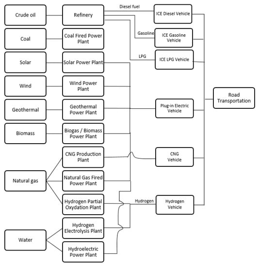
Figure 1.
Partial view of Bottom-Up Energy Modeling System’s (BUEMS’s) Reference Energy System.
As can be acknowledged from these explanations, the constraints of the model are designed to cover just about all energy related flows, interactions, limitations and requirements in the system, while featuring the critical, yet realistic linearity assumption.
4. Development of the Database and Reference Energy System
The study started with a scientific research project supported by the Scientific and Technical Research Council of Turkey [19] supported by the Ministry of Energy and Natural Resources. Several graduate theses were conducted as part of the project [18,20,21,22], through which an extensive database was developed. Data needs associated with the current situation (sub-sectoral energy demands, resource availabilities, technology and cost parameters, including capacities, vintages, economic lifetimes, efficiencies and utilization rates, investment costs, fixed/variable operational costs), as well as resource availability projections up to the end of the planning horizon, were compiled through publicly available data sources, questionnaires and expert interviews.
A compilation of demand projections at the sub-sectoral level, future prices of energy carriers and technology and cost parameters of future technologies (up to the year 2050) were problematic as even experts could not provide reliable estimates. Therefore, regarding sub-sectoral demands for future periods, it was decided to project each sub-sectoral energy demand into the future period by multiplying its current value by the estimate of the associated sectoral gross domestic product increase rate up to that period, obtained from the Turkish Statistical Institute. Official forecasts, as published under various publicly available reports, were analyzed to ensure the consistency of sectoral projections with economic and natural resource abilities and growth targets of Turkey. The consistency of sub-sectoral assumptions with overall economic growth patterns was verified by related public experts.
Regarding future prices of energy carriers, there exists a significant debate over how energy prices should be modeled. Despite a large body of empirical work, there is still much uncertainty regarding the true dynamics of energy price changes. In countries like Turkey where a major part of energy demand is met by imports, prices principally result from the interaction of world demand and supply. In 2018, 74.5% of Turkey’s primary energy supply was imported. Thereby, 88% of the country’s crude oil demand, 99.1% of its natural gas demand and 97.3% of its hard coal demand was brought into the country. In this study, price forecasts of the imported fossil fuels are based on IEA assumptions reported in the World Energy Outlook [23] whereas domestic fuels’ prices are based on the guess of experts. IEA trajectories were used to reflect expert elicitation together with the inputs from the Ministry of Energy and Natural Resources. A long-term leveling off of natural gas price growth is assumed in line with expectations for increased domestic production (shale gas from the Trace region and off-shore production from the Mediterranean) putting downward pressure on natural gas prices. Technology costs and technical characteristics that are used to compute levelized costs and a supply curve (which is stepwise because it is built up by discrete technologies). All technology parameters (efficiencies, lifetimes, investment and operating costs) are taken from the publicly available EPA (United States Environmental Protection Agency) database. The supply-side technologies are matched with energy service demands to select from each of the energy sources, carriers, and transformation technologies to produce the least-cost solution. These demand levels are modeled in this application as price insensitive, i.e., demand remains unchanged if the supply prices change and vice-versa. It was a necessary assumption for the current study as there was neither availability of information on price elasticities nor an explicit representation of the macroeconomy integrated in the employed modeling framework. This is a common approach for these kinds of bottom-up energy sector models, although presenting a weakness in terms of micro-economic foundations.
Figure 2 shows the simplified Reference Energy System. This overview provides an indication of the sectoral breakdown, together with energy flows from primary sources to final demand categories, thereby passing through various conversion, process and demand technologies. It is, however, a simplified representation as all the detail cannot be included due to size limitations: The model is comprised of 209 energy carriers, 99 demand categories and 1545 technologies.
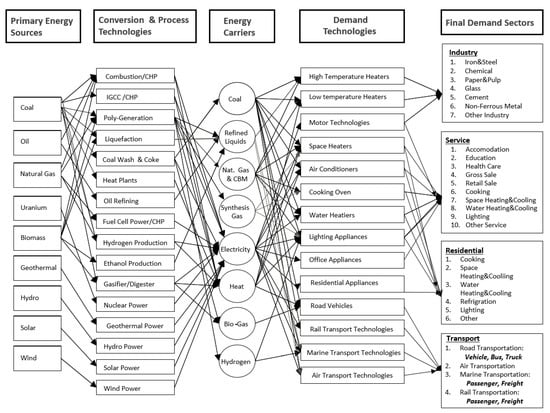
Figure 2.
The BUEMS simplified reference energy system.
In BUEMS, the transport sector is grouped into four major modes: air, maritime, rail and road transportation. These major modes are also divided into sub-modes, as shown in Figure 3.
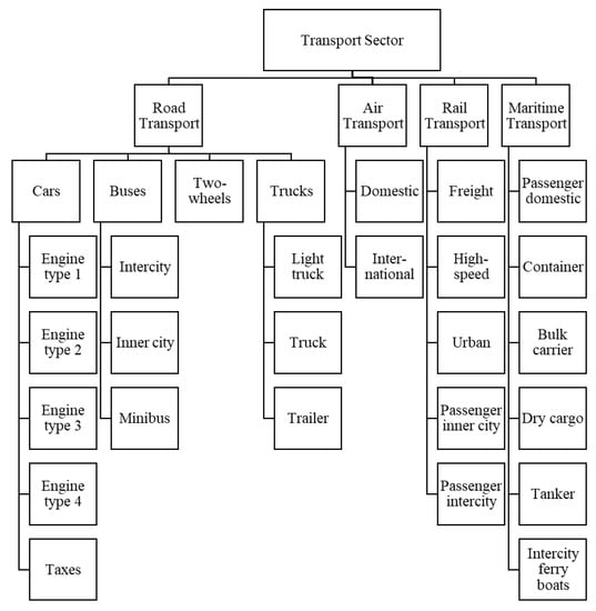
Figure 3.
Sub-modes of the transport sector in BUEMS.
For all twenty-five sub-modes, BUEMS requires total billion vehicle kilometers traveled per year as the sectoral demand data of the transport sector. This data is the most critical data for the transport sector when different policy scenarios are applied and scenario results are compared. Demand data, total billion vehicle kilometers traveled, is calculated as total distance independently of passenger number or freight amount carried on the vehicle.
Fuel efficiencies, fixed and variable operation and maintenance costs, lifetimes, residual capacities, capacity bounds, activity levels, availability factors, investment prices, investment bounds are other input requirements for transport sector technologies in BUEMS. All the data required by the model for the transport sector is compiled for the base year 2012 and year 2017 according to the gathered data. Then, data between 2017 and 2052 is estimated based on a strategic plan of MoTI (Ministry of Transport and Infrastructure) and expert consultation.
5. Model Calibration
BUEMS is calibrated according to the most recent publicly available energy and transport data for Turkey. Reference year and validation year are taken as 2012 and 2017, respectively, with model results in five-year time intervals from 2022 until 2052. The base scenario reflects the current energy flows in Turkey with its business-as-usual assumptions, together with a modest prediction for electric vehicles. The transport sector refinement, data update and calibration are based on a graduate study by [24] where further detail on model calibration can be found. Various electric vehicle diffusion and policy scenarios are carried out and results of these alternative scenarios are compared with the base scenario.
5.1. Data and Assumptions
This section describes demand data sources, their compilation and associated assumptions for the transport sector.
- Road Transport: Demand data, billion vehicle kilometers, for years 2012 and 2017 are compiled by using reports from the General Directorate of Highways (KGM) and statistics from the Statistical Institute of Turkey (TUIK) while demand data for future years are predicted based on expert consultation for all transport sub-modes in the transport sector.
- Air Transport: International flights with departures from Turkey are included in air transport demand data together with all domestic flights. Turkish Airlines Annual Reports are used to calculate total demand. In the calculation of international take-offs, only data for airlines based in Turkey were available.
- Rail Transport: Train kilometers except for rail urban are compiled from TUIK statistics and Turkish Railways Annual Statistics published by the Turkish State Railways. However, there exist no statistics related to rail urban sub-mode includes metro and tramway trains in the cities. Therefore, this information is gathered from the municipalities of the cities with metro and/or tramway infrastructure. Demand data for future years is estimated according to expert guess.
- Maritime Transport: Only domestic marine navigation is taken into consideration. Demand data for each sub-mode is calculated according to data obtained from the General Directorate of Maritime Affairs and TUIK. Demand data, billion vehicle kilometers, for future years is estimated according to expert guess.
A summary of the demand data by each of the transport modes for 2022 through to 2052, in five-year intervals, are presented in Table 1 below with details of their breakdowns in [24].

Table 1.
Demand data by mode of transportation, 2022–2052.
5.2. Electric Vehicles Consumption Data
Upper and lower bounds are set according to the prediction of consumption values for electric vehicles to obligate electric vehicles deployment in BUEMS. The behavior and effects on the energy system and emissions of electric vehicle deployment are observed under different diffusion and energy policy scenarios. Electric vehicles are differentiated into three categories: electric cars, electric buses and electric rail vehicles.
For the diffusion of electric cars, only lower bounds are used. Bounds for consumption levels of electric cars are based on expert survey results estimating 140,000 electric vehicles (EVs) to be on the road in Turkey by the year 2022—see Appendix A for the survey instrument. While this estimate is also expressed by the government, it does not appear to be realistic given the limited increase in EV charging stations and low EV sales. Also, the national electric vehicle manufacturing project has been progressing slower than anticipated. Hence, for the base scenario, the official estimate is reduced by 50%. In other words, it is assumed that there will be 70,000 EVs on the road in Turkey by the year 2022. Electricity consumption level predictions of electric cars are finalized according to the below assumptions:
- An increase of 19.1% per year in the number of electric cars.
- A consumption of 25 kWh of electricity per 100 km [25].
- An annual mileage of 15,000 km.
In consequence of the above assumptions, finalized numbers and electricity consumption levels of electric cars, which are included in BUEMS as lower bounds in the base case reference scenario (BASE), are provided together with the corresponding number of cars in Table 2 below.
Table 2.
BASE scenario electric cars’ lower electricity consumption bounds (PJ).
On the part of electric buses, both upper and lower bounds are used. To determine current numbers of electric buses, the municipalities are contacted one by one. As a result, the below assumptions and electricity consumption bounds are used for electric buses.
Assumptions for lower bounds:
- An estimation of 79 electric buses in 2022, increasing by 8% per year.
- A consumption of 135 kWh of electricity per 100 km [25].
- Annual mileage of 50,000 km.
Assumptions for upper bounds:
- An estimation of 99 electric buses in 2022, increasing by 16% per year.
- A consumption of 150 kWh of electricity per 100 km [25].
- Annual mileage of 50,000 km.
Finalized numbers and electricity consumption levels of electric buses that are included into BUEMS as upper and lower bounds are represented in Table 3 below.
Table 3.
BASE scenario electricity consumption bounds for Electric Buses (PJ).
For electric rail vehicles, upper and lower bounds are also prepared. Consumption levels of electric rail vehicles except for rail urban sub-mode are based on TCDD data. On the side of rail urban part, electricity consumption values of urban rail systems in Ankara is found from the municipality website. Then, electricity consumption calculations for other cities are obtained, as shown in Table 4.
Table 4.
BASE scenario electricity consumption bounds for Rail Vehicles (PJ).
5.3. Scenario Definitions
For the base scenario (“BASE”) definition, the current energy system of Turkey is represented with its business-as-usual assumptions, together with a modest prediction on minimal diffusion of EVs, as shown in Table 2, Table 3 and Table 4. In addition to BASE, various alternative scenarios are defined to evaluate the impacts of alternative policies. These are summarized in Table 5 and further described in detail as follows:
Table 5.
Scenario Summary.
MOREECAR: In addition to the BASE scenario, a more rapid distribution of EVs is assumed in the MOREECAR scenario, which—in line with official estimates—starts with 140 thousand electric cars in 2022. The assumption of 140 thousand e-cars in 2022 is based on the official declaration by the Minister of Industry and Technology [26]. In this scenario, the electricity consumption levels of electric cars, included in BUEMS as lower bounds, are as follows. All assumptions other than the lower bounds on electric cars, as depicted in Table 6, are the same as in the BASE scenario.
Table 6.
MOREECAR scenario electric cars’ lower electricity consumption bounds (PJ).
NONEWCOAL_E: In this scenario coal based electricity generation is limited starting from the year 2027 as no new coal fıred power plant is constructed after 2027. Thus it is made sure that the growing electricity demand due to the deployment of EVs is not coming from new coal-fired power plants. Accordingly, the electricity sector grows with renewables and natural gas fired power generation instead of coal. All assumptions other than the construction ban on coal fired power plants are the same as in the BASE scenario. The year 2027 has been chosen for a ban on new coal fired power generation as it is the first model year coming after 2023. The official power sector strategy is to utilize all domestic coal reserves by the year 2023 [27]. The utilization of indigenous coal reserves is part of the policy priority to reduce import dependence, and a ban on new coal-fired power generation is possible once domestic resources are exploited.
NODIESEL_T: A ban on new diesel cars is used as an alternative policy instrument to assure an accelerated diffusion of electric cars. The UK, for example, announced a ban on the sales of new diesel and gasoline powered cars in 2035. The impacts of such a policy on the diffusion of electric cars are explored under the NODIESEL scenario. The introduction of new diesel cars and buses is banned in this scenario starting from the year 2027, thereby restricting coal based electricity generation so as to direct the transport sector’s incremental electricity demand due to the ban towards less carbon-intensive energy sources. The ban on diesel fueled vehicles expanding rapidly in Europe is expected to affect Turkey gradually with a stop in the manufacturing of diesel cars by 2030 [28]. The scenario bans the introduction of new diesel vehicles in 2027, which is the latest model year before the expected stop of manufacturing. All assumptions other than the diesel ban on new cars and restriction of coal-fired power generation, as depicted in Table 7, are the same as in the BASE scenario.
Table 7.
Consumption bounds for coal-fired power generation in the NODIESEL_T scenario (PJ).
ISTBUS: This scenario is created on the consideration of what will happen if all the buses in Istanbul are electric vehicles by the year 2027. Therefore, according to the inner city bus transport data of Istanbul, the electric buses’ bounds are revised. It should be noted that the annual growth rate of electricity consumption bounds from 2027 until 2052 averages 15.4%, as shown in Table 8. The rate of increase in the number of buses gets slightly higher due to efficiency increase over time, reaching between 190,000 and 622,787 e-buses by 2052 with a 10–17% average annual increase. Also, coal fired power plants are restricted in the ISTBUS scenario to direct the growing electricity demand of electric buses to renewable energy. The restrictions on coal-fired power generation are the same as in the NODIESEL_T scenario, as shown in Table 9. The Istanbul Municipality has announced plans to convert all inner city bus transport to electricity by the year 2030 [29]. The scenario assumes all bus transport in Istanbul to become electric by 2027, which is the latest model year before the planned transformation.
Table 8.
Electricity consumption bounds for electric buses in the ISTBUS scenario (PJ).
Table 9.
Consumption bounds for coal-fired power generation in the ISTBUS scenario (PJ).
All assumptions other than the bounds on electric buses and coal-fired power generation as depicted in Table 8 and Table 9 are the same as in the BASE scenario.
It should be noted that when the lower bounds are binding, for example, Table 6, the presented results are the low bound results, while the results with the upper bounds significance, Table 7 and Table 9, we present the upper bound fixed results as such. Table 8 is the exception with the upper and lower bounds results presented.
In the following section, scenario results will show that with the increase in electric cars, CO emissions from electricity generation rise while transport sector emissions decrease. The rise in emissions is essentially due to increased coal-fired power generation. Therefore, in order to limit the growth of emissions, various scenarios restricting coal use were defined along with scenarios with CO bounds and CO taxes. The carbon tax (50$/ton CO) is applied on the transport sector and electricity sector both individually and simultaneously under alternative scenarios.
CO2TAX50_T: In this scenario, an emission tax of $50 per ton of CO is introduced in transportation starting from the year 2032. The tax is applied on all modes of transportation, yet applied on the transport sector only. The tax amount of $50 per ton of CO is pretty much in line with assumptions and findings in the scientific literature. For example, a fixed tax trajectory was set such that the tax begins in 2020 at either $25 or $50 and rises at either 1% or 5% per year [30]. Starting at the $50 level without further escalation is assumed in this scenario. All assumptions other than the emission tax are the same as in the BASE scenario.
CO2TAX50_E: In this scenario, an emission tax of $50 per ton of CO is introduced in power generation starting from the year 2032. The tax is applied in the electricity sector only. The tax amount of $50 per ton of CO is in line with assumptions and findings in the scientific literature as mentioned in the previous scenario description. All assumptions other than the emission tax are the same as in the BASE scenario.
6. Model Results
The total energy consumption of transportation includes electricity, petroleum, diesel, biodiesel, hydrogen, jet fuel, CNG, LPG, ethanol and methanol as fuel types, as shown in Figure 4. According to the results of the base scenario, diesel fuel is the dominant fuel from the beginning of the planning horizon, 56.4% in 2012 and 53.4% in 2017. However, its share in total transport energy consumption decreases over time, reducing to 31.5% in 2047 and 22.5% in 2052 being essentially substituted by gasoline fueled vehicles and EVs. The increase in the use of petroleum use is a result of the substitution of gasoline for diesel fueled vehicles and the increase in the demand of residual fuel oil used in ships, together with the rapid increase in overall transport demand. Its rising share indicates the long-run price competitiveness of petroleum. Electricity consumption in transportation gradually increases because of electric car deployment with a share of 0.3% in 2012, 0.5% in 2017, 6.3% in 2047 and 13.8% in 2052. Hydrogen fuel, which has no incentive in the model like plug-in EVs, gets involved at the end of the planning horizon only with a consumption of 1.6 PJ in 2052. While jet fuel and petroleum consumption continue to grow depending on the increase of transport demand, methanol consumption decreases for each period. Lastly, LPG, which is being used because of economic reasons in Turkey as it is cheaper than other alternatives being subsidized, drops over time from a considerable share of 15.49% in 2012, becoming zero by the year 2047 due to a considerable increase in electric cars.
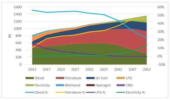
Figure 4.
Energy consumption of the transport sector by fuel type: BASE scenario.
The electricity consumption of the transport sector is dominated by electric cars. While it is negligibly small in 2012 and only 0.1 PJ in 2017, it reaches 75.2 PJ in 2047 and 180.6 PJ in 2052, as shown in Figure 5.
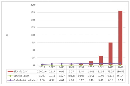
Figure 5.
Electricity consumption of the transport sector by vehicle type: BASE scenario.
CO emissions are increasing in all scenarios; total emissions of the BASE scenario skyrocketed from 359,280 kton in 2017 to 1,408,500 kton in 2052, which is almost quadruple. Transport sector emissions are increasing from 65.6 kton in 2017 to 83.1 kton in 2052 implying a 26.7% increase. Most interestingly, the more EVs are deployed, the higher the total emissions, as can be observed by comparing the MOREECAR and BASE scenarios in Figure 6. This is because of increased coal usage for power generation; therefore it is essential to limit the expansion of coal. That is why all other scenarios have a limitation or policy in place to reduce coal usage. When the results of these scenarios are investigated it is seen that emissions decrease by 0.4%, 4%, 11%, 29% and 51% in 2052 for the CO2TAX50_E, ISTBUS, MOREECAR, NODIESEL_T and CO2TAX50_T scenarios, respectively, in comparison to the BASE scenario.
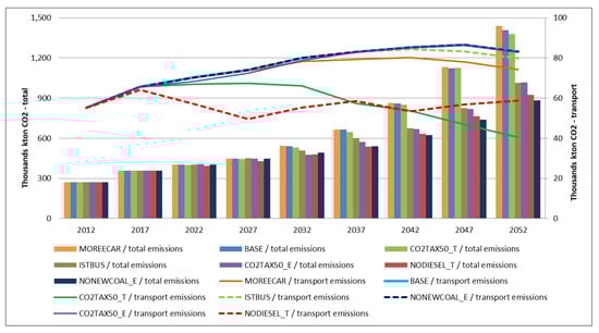
Figure 6.
Total and transport sector emissions by scenario.
Turkey’s skyrocketing total emissions are almost proportional to the change in coal-fired power generation, as can be observed from Figure 7. Total emissions increase by 1049 Mton (from 359 Mton in 2017 to 1408 Mton in 2052), of which 49.5% comes from increased coal-fired power generation. In 2052, coal-fired power generation amounts to 3721 PJ in the BASE and 3939 PJ in the MOREECAR scenario. It reduces to 1520 PJ, 708 PJ and 440 PJ in the CO2TAX50_E, ISTBUS and NONEWCOAL_E scenarios, respectively. Accordingly, in terms of emission reduction, the most effective policy options, ordered by reduction amount, are (i) banning new investment in coal-fired power plants, (ii) making bus transportation in Istanbul electric, and (iii) introducing a carbon tax on electricity generation. However, are these options cost-effective? The next section compares the system-wide cost implications of the scenarios.
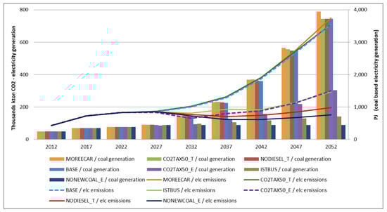
Figure 7.
Emissions from electricity generation and coal-based electricity generation levels by scenario.
Lifetime emissions and lifetime cost values, discounted to the year 2019, are depicted in Figure 8. It can be seen that all alternative scenarios have lower total emissions than the BASE scenario except for MOREECAR. Also, all of them have higher total system cost compared to the BASE scenario except for NODIESEL_T. In other words, the NODIESEL_T scenario has lower lifetime emissions and lower lifetime costs—a profitable decarbonization option pointed out by the model. It should be noted that the BASE scenario includes lower bounds for diesel vehicles so as to yield the most likely reference path under business-as-usual conditions. Obviously, this business-as-usual pathway with increasing diesel vehicles is not the cheapest one as a lower cost pathway emerges when there is a ban on new diesel fueled vehicles. The diesel consumption in the transport sector reduces drastically as a result of the ban on new vehicles, yet does not vanish until the end of the lifetime of the existing diesel-fueled vehicle stock. The diesel gap between the BASE scenario and NODIESEL_T reduces over time as the share of diesel fuel declines in the long term in the BASE scenario anyway. The diesel consumption of the transport sector in the year 2027 is 573.48 PJ in the BASE scenario versus 215.69 PJ in the NODIESEL_T scenario. Then, in year 2052, diesel consumption gets 306.05 PJ in scenario BASE and 113.17 PJ in the NODIESEL_T scenario.
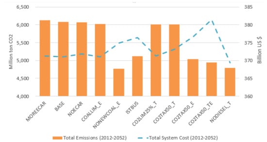
Figure 8.
Total emissions and total system cost by scenario throughout the planning horizon.
While NODIESEL_T offers a win-win opportunity, the MOREECAR scenario indicates a lose-lose option: it has a higher total system cost and higher total emissions than the BASE scenario. This is because the growing electricity demand due to increased e-mobility is met by coal-fired electricity generation. Therefore, in the absence of decarbonization in electricity generation, the diffusion of e-mobility is not sustainable. It helps only to reduce emissions on the road while that reduction is offset by increased emissions from electricity generation.
The ratio of lifetime cost changes to lifetime CO changes, referred to as marginal abatement cost, is shown in Table 10. The win-win NODIESEL_T scenario indicates a profit of 1.29$ per ton CO reduced. The lose-lose MOREECAR scenario on the other hand has no marginal abatement cost because its emissions are higher than in the BASE scenario, hence no abatement.
Table 10.
Lifetime Marginal Abatement Costs (cost increase/emission savings).
When scenarios are ranked according to lifetime marginal abatement cost, the lowest cost options are associated with the electricity sector (NONEWCOAL_E and CO2TAX50_E), followed by urban e-bus (ISTBUS). Carbon taxation in transportation (CO2TAX50_T) appears to be the least cost-effective policy option.
Table 11 presents the periodical breakdown of the abatement cost figures for each scenario. It can be observed that the abatement declines over time in all scenarios except the win-win scenario NODIESEL_T where profit declines. In the NODIESEL_T scenario there is an adaptation process for shifting away from diesel vehicles, which is highly profitable in the short run as explained previously, and diminishes in the longer term when the shift is completed. In the other scenarios, the initial investments into low-carbon technologies induce high up-front costs but lower operating and maintenance costs, essentially due to renewables, results in savings in the longer term. It can be seen that a CO tax on electricity generation (CO2TAX50_E) is initially profitable as well, has an abatement cost of 30.66 $/ton CO in 2032 (the year when carbon tax is launched), which gradually decreases thereafter.
Table 11.
Overall CO abatement costs by scenario.
The primary energy supply mix composition of energy technologies for the BASE and alternative scenarios are depicted in Figure 9 and Figure 10, respectively.
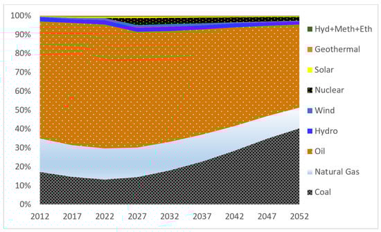
Figure 9.
Primary energy supply mix in the BASE scenario.
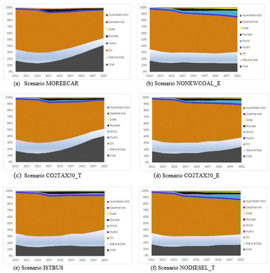
Figure 10.
Primary energy supply mix in the alternative scenarios.
7. Sensitivity Analysis
Transport sector demand data and the cost of EVs are among the most important parameters affecting scenario results in this study. Therefore, the sensitivity analysis focuses on these two parameters, thereby elaborating on their impacts on CO emissions and energy system costs. It is found that the results are much more sensitive to demand than to the cost of EVs. According to Figure 11, a 20% rise in transport sector demand causes a 0.7% increase in total emissions while 20% rise in EV cost causes less than 0.1% increase. On the other hand, a 20% fall in EV cost reduces emissions by 0.2% while a 20% fall in transport sector demand provides a 0.7% decrease.
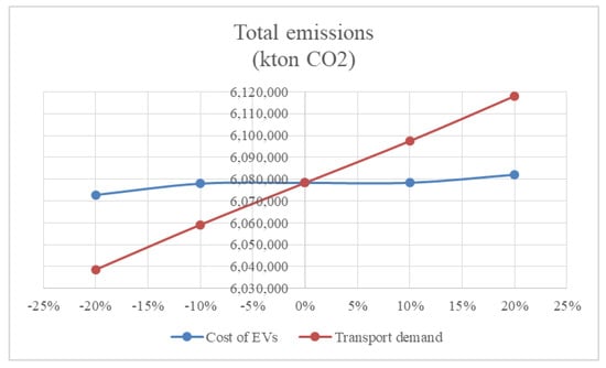
Figure 11.
Total emissions change with different data for transport sector demand and cost of electric vehicles (EVs) in the base scenario.
As can be seen from Figure 12, a 20% rise in transport sector demand causes a 1.5% increase on total system cost while a 20% rise in EV cost causes a 0.13% increase. On the other hand, 20% fall in EV cost provides a 1.47% decrease in total system cost while a 20% fall in transport sector demand leads to a 0.17% decrease.
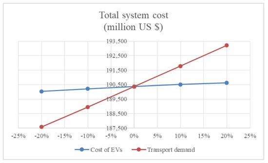
Figure 12.
Total system cost change with different data for transport sector demand and cost of EVs in the base scenario.
8. Conclusions
Evaluation of electric vehicle deployment with respect to energy and environmental impacts is a multilateral task in need of a technologically detailed multisectoral analysis. To evaluate the long-term impacts of alternative policies, the bottom-up model BUEMS has been used and calibrated under various scenarios according to the most recent Turkish energy and transport sector data. All the complex relationships of producing, transforming, transmitting and/or supplying energy sources according to the useful demand characteristics are represented with great technological detail.
Model results highlight win-win policy options that lead to profitable decarbonization. In particular, it is found that a ban of diesel fueled vehicles reduces lifetime emissions as well as lifetime costs. Hence, the diesel ban scenario results in negative abatement costs over the planning horizon. This finding is in support of all the urban policies being implemented worldwide to get rid of diesel fueled vehicles in the cities, which has become very popular especially after the Dieselgate scandal in 2015. German cities started introducing bans on older diesel vehicles with the court several years ago. Major cities like Paris and London are now following this trend, which leads to profitable decarbonization in Turkey. Therefore, while there still is no such agenda, Turkish municipalities should consider introducing a ban on diesel fueled vehicles to exploit the profitable emission reduction potential. Besides banning diesel fueled vehicles, Turkish municipalities should also consider introducing electric buses for public transportation as pointed out by model results. The marginal cost of emission reduction through e-buses is much lower than through other policy measures like carbon taxation in transport.
It should be noted that the electricity sector plays a crucial role on the sustainability of e-mobility. It is found that the elimination of emissions on the road through e-mobility is more offset by emissions from power plants if electricity is generated by coal. This is a particularly important finding for a country like Turkey, which has both ambitious e-mobility diffusion plans as well as policy priority goals on the utilization of domestic coal reserves for electricity generation. From a sustainability point of view, these two do not go hand in hand as pointed out by the scenario results. Decarbonization of electricity generation is therefore of primary importance for electrification of transportation. It is found that a ban on new coal-fired power generation is a cost-effective way for reducing emissions in the electricity sector. Introducing an emission tax in the electricity sector is about five-fold more cost effective than introducing an emission tax in transportation (5.47 $/ton CO in electricity vs. 27.37 $/ton CO in transport for 50 $/ton CO emission tax).
For further research, model resolution can be increased so as to introduce a daily load duration curve and allow for optimization of instantaneous charging needs with network supply/demand balance. Also, the model can be developed into a price-elastic version to reflect the impact of price changes on the demand for electricity, other energy sources and technology choices. Furthermore, the storage potential of renewable power generation or their intermittent nature [31] can be explored in more detail using a stochastic model extension.
Author Contributions
Conceptualization, G.K. and C.C.; methodology, G.K. and E.S.; validation, J.D. and E.S.; resources, J.D. and E.S.; data curation, G.K. and C.C.; writing–original draft preparation, G.K. and C.C.; writing–review and editing, J.D. and E.S.; project administration, G.K., J.D. and E.S.; funding acquisition, G.K. and E.S. All authors have read and agreed to the published version of the manuscript.
Funding
This research was funded by the Scientific and Technical Research Council of Turkey under Scientific Research Project #104M348. This research was also partially funded by the United States National Science Foundation under Award No. 1847077.
Acknowledgments
The authors would like to acknowledge the support from Bogazici University under Scientific Research Project BAP12281, as well as the Fulbright Commission under Grant #FY-2019-TR-SS-17 for featuring the international collaboration.
Conflicts of Interest
The authors declare no conflict of interest. The funders had no role in the design of the study; in the collection, analyses, or interpretation of data; in the writing of the manuscript, or in the decision to publish the results.
Abbreviations
The following abbreviations are used in this manuscript:
| CO | Carbon dioxide |
| USA | United States of America |
| EV | Electric Vehicle |
| BUEMS | Bottom-Up Energy Modeling System |
| IEA | International Energy Agency |
| IPCC | Intergovernmental Panel on Climate Change |
| V2G | Vehicle to Grid |
| CV | Conventional gasoline Vehicle |
| HEV | Hybrid Electric Vehicle |
| PEV | Plug-in Electric Vehicle |
| LDV | Light-Duty Vehicle |
| GCAM | Global Change Assessment Model |
| TIMES | The Integrated MARKAL-EFOM System |
| LEAP | Long-range Energy Alternatives Planning model |
Appendix A. Survey Instrument

Figure A1.
Electric vehicle deployment projection survey in Turkey.
Figure A1.
Electric vehicle deployment projection survey in Turkey.

References
- IEA. CO2 Emission from Fuel Combustion, Statistics Report. Technical Report. 2019. Available online: https://www.iea.org/reports/co2-emissions-from-fuel-combustion-2019 (accessed on 30 July 2020).
- Pachauri, R.K.; Allen, M.R.; Barros, V.R.; Broome, J.; Cramer, W.; Christ, R.; Church, J.A.; Clarke, L.; Dahe, Q.; Dasgupta, P.; et al. Climate Change 2014: Synthesis Report. Contribution of Working Groups I, II and III to the Fifth Assessment Report of the Intergovernmental Panel on Climate Change; World Meteorological Organization (WMO): Geneva, Switzerland, 2014; Available online: https://epic.awi.de/id/eprint/37530/1/IPCC_AR5_SYR_Final.pdf (accessed on 30 July 2020).
- IPCC. Climate Change 2014, Mitigation of Climate Change. Contribution of IPCC AR5 WG3 2014: Working Group III to the Fifth Assessment Report of the Intergovernmental Panel on Climate Change; Cambridge University Press: Cambridge, UK; New York, NY, USA, 2014. [Google Scholar]
- Shittu, E.; Parker, G.; Jiang, X. Energy technology investments in competitive and regulatory environments. Environ. Syst. Decis. 2015, 35, 453–471. [Google Scholar] [CrossRef]
- Shittu, E. Energy technological change and capacity under uncertainty in learning. IEEE Trans. Eng. Manag. 2013, 61, 406–418. [Google Scholar] [CrossRef]
- Kamdem, B.G.; Shittu, E. Optimal commitment strategies for distributed generation systems under regulation and multiple uncertainties. Renew. Sustain. Energy Rev. 2017, 80, 1597–1612. [Google Scholar] [CrossRef]
- Deluque, I.; Shittu, E.; Deason, J. Evaluating the reliability of efficient energy technology portfolios. EURO J. Decis. Process. 2018, 6, 115–138. [Google Scholar] [CrossRef]
- Alexander, M.; Tonachel, L. Projected Greenhouse Gas Emissions for Plug-in Electric Vehicles. World Electr. Veh. J. 2016, 8, 987–995. [Google Scholar] [CrossRef]
- UNFCCC. National Inventory Report Turkey. 2019. Available online: https://unfccc.int/documents/19481 (accessed on 4 August 2020).
- Zhang, H.; Chen, W.; Huang, W. TIMES modelling of transport sector in China and USA: Comparisons from a decarbonization perspective. Appl. Energy 2016, 162, 1505–1514. [Google Scholar] [CrossRef]
- Wu, D.; Aliprantis, D.C. Modeling light-duty plug-in electric vehicles for national energy and transportation planning. Energy Policy 2013, 63, 419–432. [Google Scholar] [CrossRef]
- Tsita, K.G.; Pilavachi, P.A. Decarbonizing the Greek road transport sector using alternative technologies and fuels. Therm. Sci. Eng. Prog. 2017, 1, 15–24. [Google Scholar] [CrossRef]
- Paladugula, A.L.; Kholod, N.; Chaturvedi, V.; Ghosh, P.P.; Pal, S.; Clarke, L.; Evans, M.; Kyle, P.; Koti, P.N.; Parikh, K.; et al. A multi-model assessment of energy and emissions for India’s transportation sector through 2050. Energy Policy 2018, 116, 10–18. [Google Scholar] [CrossRef]
- Li, F.; Cai, B.; Ye, Z.; Wang, Z.; Zhang, W.; Zhou, P.; Chen, J. Changing patterns and determinants of transportation carbon emissions in Chinese cities. Energy 2019, 174, 562–575. [Google Scholar] [CrossRef]
- Lazarou, S.; Christodoulou, C.; Vita, V. Global Change Assessment Model (GCAM) considerations of the primary sources energy mix for an energetic scenario that could meet Paris agreement. In Proceedings of the 2019 54th International Universities Power Engineering Conference (UPEC), Bucharest, Romania, 3–6 September 2019; pp. 1–5. [Google Scholar]
- Lazarou, S.; Markovic, F.; Dagoumas, A. Energy and climate policy with the GCAM model: Assessing energy sources and technology options. Int. J. Renew. Energy Res. (IJRER) 2018, 8, 2299–2309. [Google Scholar]
- Karali, N. Design and Development of a Large-Scale Energy Model. Ph.D. Thesis, Bogazici University, Istanbul, Turkey, 2012. [Google Scholar]
- Işık, M. Energy, Economy and Environment Integrated Large-Scale Modeling and Analysis of the Turkish Energy System. Ph.D. Thesis, Bogazici University, Istanbul, Turkey, 2016. [Google Scholar]
- Tubitak. Development of the Boğaziçi University Energy Modeling System and Evaluation of Greenhouse Gas Emission Restrictions on the Turkish Economy; Technical Report; Scientific and Technical Research Council of Turkey: Istanbul, Turkey, 2018. [Google Scholar]
- Tetik, E. Turkish Electricity Sector: A Bottom-Up Approach. Master’s Thesis, Isik University, Istanbul, Turkey, 2017. [Google Scholar]
- Günel, G. Analysis of CO2 Emission Reduction, Energy and Economy Interactions in Turkey Using BUEMS-MACRO. Master’s Thesis, Boğaziçi University, Istanbul, Turkey, 2018. [Google Scholar]
- Yıldırım, I. Energy Policy Analysis with the Boğaziçi University Energy Modeling System BUEMS: Prospects for the Diffusion of Renewable Energy Tecnologies and Utilization of Domestic Coal Reserves in Turkey. Master’s Thesis, Boğaziçi University, Istanbul, Turkey, 2019. [Google Scholar]
- IEA. World Energy Outlook 2009. Available online: http://large.stanford.edu/courses/2013/ph241/roberts2/docs/WEO2009.pdf (accessed on 30 July 2020).
- Canaz, C. Transport Sector Energy Use, Electric Vehicle Deployment and CO2 Emissions in Turkey: An Evaluation Using the Boğaziçi University Energy Modeling System. Master’s Thesis, Boğaziçi University, Istanbul, Turkey, 2019. [Google Scholar]
- IEA. Global EV Outlook 2018: Towards Cross-Modal Electrification. Technical Report. 2018. Available online: https://www.oecd.org/publications/global-ev-outlook-2018-9789264302365-en.htm (accessed on 30 July 2020).
- Erdem, U. Varank’a Göre 2022’de 140 bin Elektrikli Araç Yollara çıkacak. 2019. Available online: https://www.hurriyet.com.tr/ekonomi/varanka-gore-2022de-140-bin-elektrikli-arac-yollara-cikacak-41109629 (accessed on 30 July 2020).
- MENR. Electric Energy Markets and Supply Security Strategy Document. 2009. Available online: https://www.enerji.gov.tr/File/?path=ROOT (accessed on 30 July 2020).
- Soczu. Avrupa’daki dizel Yasakları Türkiye’yi de Etkileyecek. 2020. Available online: https://www.sozcu.com.tr/2020/otomotiv/avrupadaki-dizel-yasaklari-turkiyeyi-de-etkileyecek-5566743/ (accessed on 30 July 2020).
- Milliyet. Istanbul Otobusleri ’Elektrik’lenecek. 2016. Available online: https://www.milliyet.com.tr/gundem/istanbul-otobusleri-elektrik-lenecek-2355216 (accessed on 30 July 2020).
- Barron, A.R.; Fawcett, A.A.; Hafstead, M.A.; McFarland, J.R.; Morris, A.C. Policy insights from the EMF 32 study on US carbon tax scenarios. Clim. Chang. Econ. 2018, 9, 1840003. [Google Scholar] [CrossRef] [PubMed]
- Jiang, X.; Parker, G.; Shittu, E. Envelope modeling of renewable resource variability and capacity. Comput. Oper. Res. 2016, 66, 272–283. [Google Scholar] [CrossRef]


© 2020 by the authors. Licensee MDPI, Basel, Switzerland. This article is an open access article distributed under the terms and conditions of the Creative Commons Attribution (CC BY) license (http://creativecommons.org/licenses/by/4.0/).