Abstract
Voids that are formed by gas injection in a packed bed play an important role in metallurgical and chemical furnaces. Herein, two-phase gas–solid flow in a two-dimensional packed bed during blast injection was simulated numerically. The results indicate that the void stability was dynamic, and the void shape and size fluctuated within a certain range. To determine the void morphology quantitatively, a probabilistic method was proposed. By statistically analyzing the white probability of each pixel in binary images at multiple times, the void boundaries that correspond to different probability ranges were obtained. The boundary that was most appropriate with the simulation result was selected and defined as the well-matched void boundary. Based on this method, the morphologies of voids that formed at different gas velocities were simulated and compared. The method can help us to express the morphological characteristics of the dynamically stable voids in a numerical simulation.
1. Introduction
Voids that are formed by gas injection in a packed bed are critical in various applications, such as moving-bed coal gasifiers [1], blast furnaces [2] and COREX melting gasifiers [3]. For example, the tuyere raceway in the lower part of the blast furnace is exactly the void that is formed by a high-pressure air blast, which provides heat and a reducing gas for reaction in the upper part. The void morphology (i.e., shape and size) is believed to be an important factor to determine the distribution of the reducing gases and heat [4]. Therefore, an exploration of the void morphology has important implications for controlling the gas distribution and reactions [5].
In past decades, void formation has been investigated extensively by different experimental techniques and by numerical simulation [4,6,7,8,9]. For example, based on a dimensional analysis, Rajneesh et al. [10,11] established a cold model experiment and proposed two void correlations to determine the void depth and height. X-ray computed tomography (CT) was used by Nogami et al. [12] to measure the three-dimensional (3D) shape and structure of the void by evaluating the differences between two successive CT images. Di et al. [13,14] established a semicircle model with a 1:20 scale according to the prototype of one factory, and derived the formula to determine the void surface area on the basis of fractal theory and coke particle velocity contour. Lu et al. [15] used an optical method to study the void formation in a 3D packed bed, and concluded that the void was closer to an ellipsoid.
Because of experimental limitations in terms of high construction costs, a numerical simulation that uses a continuum approach or a discrete-element method (DEM) has become necessary to study the void formation process for realistic processes in advance. In the continuum approach, the fluid and particle phases are considered continuous media. Rangarajan et al. [16] used a two-fluid modeling method to study the void formation, and reported that the gas velocity influences the void size. In general, the continuum approach is suitable for large-scale computations, but finds it difficult to obtain detailed microscopic dynamic information on the void. The discrete-based approach can solve this difficulty. For example, Tsuji et al. [17,18,19] proposed a coupling method using DEM and a continuum approach to study plug conveying in a pipe. Xu et al. [20] used combined continuum and discrete modeling to simulate gas–solid flow in packed beds by establishing a two-dimensional (2D) slot model. Miao et al. [21] coupled computational fluid dynamics (CFD) and DEM to investigate the formation of voids in a full-scale 2D slot model, and found that three void types formed at different gas velocities, such as a clockwise circulating void (at a low gas velocity), an anti-clockwise circulating void (at a medium gas velocity) and a plumelike void (at a high gas velocity). With CFD–DEM, Sun et al. [3] studied the void formation in COREX by analyzing the movement and phase volume fraction of particles, and reported that it took 4 s for the void to reach a steady state.
Previously, the void morphology was usually determined as a static instantaneous value in literature [22]. In reality, however, the morphology of void changes with time. Umekage et al. [23] reported that the void morphology changed before steady state was reached. Santana et al. [24] observed that the void oscillated alternately from t = 1.3 s to t = 3 s, and stabilized after t = 4.0 s macroscopically for a 2D rectangular geometry model. Although the void tended to be stable macroscopically after a period, the void is likely to fluctuate and maintain a dynamic stability. However, the void morphology during the macroscopic stable stage remains unclear.
In this work, we established a 2D two-phase gas–solid flow model based on CFD–DEM to simulate void formation in a packed bed. A cold experiment was conducted to verify the modeling. In the simulation, we found that the void morphology was under a dynamically stable condition even after the macroscopically stable stage from our simulation results. We proposed a probabilistic method to determine the exact void morphology by analyzing each pixel in the obtained simulation images with time. To analyze the feasibility of this probabilistic method, the voids that formed for a series of gas velocities were studied. This work provides an important strategy for determining the void morphology in various applications.
2. Materials and Methods
2.1. Modeling
2.1.1. Particle Movements Described in DEM
Particle movement in the packed bed was simulated by DEM (EDEMTM, version 2018, DEM solutions, Edinburgh, UK), and the collision between particles was considered with the soft ball model that was proposed by Cundall [25]. The governing equations for translational and rotational motion of particle i are [26],
where mi, vi, ωi and R are the mass, translational velocities, rotational velocities and radius of particle i, respectively. Fpf,i, Fcn,ij, Fct,ij, Fdn,ij, Fdt,ij and mig are the particle fluid interaction force, normal contact force, normal damping force, tangential contact force, tangential damping force and gravitational force of particle i, respectively. Ii is the moment of inertia of particle i. The torque acting on particle i includes two components: torque by tangential forces Mt,ij and rolling friction torque Mn,ij [26]. The detailed information of the forces and torques acting on particle i can be found in Appendix A.
2.1.2. Governing Equations for Gas Phase in CFD
For the gas phase, the CFD method (FLUENT) is used to determine the flow field. The gas flow is described by Navier–Stokes equations, including the standard k-ε turbulence model [27], which can be written as,
where ε is the void fraction, ρ, u, μ and p represent the bulk density, velocity vector, viscosity and pressure of the fluid, respectively; Vi represents the volume of particle I; Vcell represents the volume of a CFD mesh cells and S is the momentum sink, which is the sum of all gas drag forces in the grid.
2.1.3. The Coupling of Particle and Gas
The CFD–DEM coupling module was used to couple the DEM simulation with CFD. At each time step, the DEM transmits information to the CFD model, including the volume fraction, position and velocity of the individual particles. In the CFD simulation, the momentum sink S (the sum of all gas drag forces in the grid) is added to each of the mesh cells to represent the effect of momentum transfer from the DEM particles. The momentum sink can be expressed as:
where FD is the force on particle i in an iteration from the fluid and n is the number of particles in a single CFD mesh cell.
Momentum coupling would lead to an additional gas drag force on the particles. The drag force on particles (FD) was calculated according to Ergun [28] and Wen & Yu [29] in the simulation,
where vi denotes the solid velocity vectors and β is described by,
where CD is the resistance coefficient, which can be determined based on the Reynolds number Re.
2.1.4. Simulation Conditions and Procedure
A 2D slot model was used to simulate the void formation in a packed bed via the CFD–DEM approach. As shown in Figure 1, the 2D slot model is composed of a rectangular solid slot and a tube at the left wall (i.e., the tuyere, which is simplified as a square tube here). The cell size is 44.3 mm. The 88.6 mm × 88.6 mm square tube with a depth of 300 mm was inserted as a gas entrance.
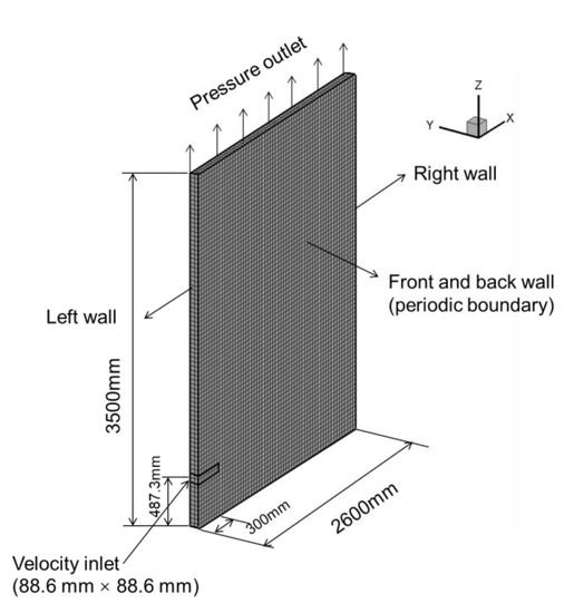
Figure 1.
Two-dimensional slot model.
During the simulation, a certain number of 40-mm-diameter spherical particles was pre-charged first from the top of the model. The particle/cell size ratio is about 1.1/1, and the particle size is slightly smaller than the cell size. The density, material shear modulus and Poisson’s ratio of the particle were 1000 kg/m3, 0.1 GPa and 0.21, respectively. Other parameters that were used in the simulation are shown in Table 1. When all pre-charged particles had settled, the gas with a density of 0.716 kg/m3 and a viscosity of 1.88 × 10⁻⁵ kg/(m·s) was injected into the packed bed at a constant 232 m/s. The gas outlet at the top was set as the boundary condition of the pressure outlet. The front and rear walls were set with periodic boundary conditions. The left and right walls were solid walls. In the CFD-DEM simulation, the time steps is 5 × 10⁻⁵ s in DEM solution and 4 × 10⁻⁵ s in CFD solution.

Table 1.
Parameters used in the simulation.
2.2. Experiment to Verify Mathematical Modeling
A cold experiment was conducted to verify the modeling. The experimental designs were based on the similarity principle, including the geometry, and flow similarity for the Froude number [30]: and . On the basis of a geometry similarity principle, a slot experimental model was designed with a 1:10 scale compared with the 2D slot model that was used in the simulation. Based on the flow similarity principle, the gas with a density of 1.23 kg/m3 and a dynamic viscosity of 1.78 × 10⁻⁵ kg/(m·s) was injected into the tuyere at 20 m3/h. Polymethyl methacrylate (PMMA) particles with a stacking angle of 35–45° and a bulk density of 1000 kg/m3 were used as the model particles. The equivalent diameter of the PMMA particles ranged from 3 to 4 mm. Detailed experimental information is provided in Appendix B.
2.3. Probabilistic Method to Determine Void Morphology
Based on the above CFD–DEM approach, void formation in a packed bed can be evaluated by simulation. We propose a new approach to determine the void morphology based on a probabilistic method by analyzing each pixel in the obtained simulation images of the void. As shown in step 1 of Figure 2, at a certain time t = 2.55 s, the simulation images were converted to gray images using the ‘Rgb2gray’ function by MATLAB. Subsequently, the gray images were changed to binary images using the ‘graythesh’ function by finding an appropriate threshold value of the image based on the Otsu method [31].
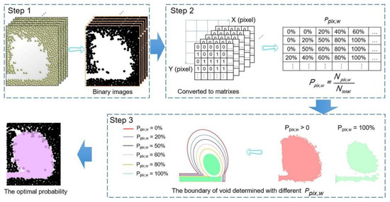
Figure 2.
Probability method steps.
Because the original image is intercepted according to the resolution of 1280 × 960 of DEM derived image, the derived matrix is 1280 × 960. In these binary images, the black and white areas represent particles and voids, respectively. Afterwards, as shown in step 2, these binary images are exported as matrixes, and contain 0 (black) or 1 (white). Then, the number of 1 (white) at each element in all the matrixes is determined, and the probabilities of the white (Ppix,w) for each pixel in the images is calculated by,
where Npix,w and Ntotal are the number of whites at each pixel and the total number of samples, respectively.
As shown in step 3, when the images with Ppix,w matched well with the void that was obtained in the simulation, this probability can be used to determine the void size. To verify the probability method, the voids that formed under various gas velocities (i.e., 168 m/s, 184 m/s, 200 m/s, 216 m/s) were studied.
3. Results
3.1. Verification of the Modeling
A mathematical model was verified by a cold experiment. Figure 3 shows the void formation in the simulation (Figure 3a) and experiment (Figure 3b) under the same conditions. As shown in Figure 3a, after gas injection, a void with a plume-like shape (the void height was greater than its depth) formed, which is consistent with previous studies [21]. The packed bed, particle and blast properties were all checked. The blast velocity was more than 1 m/s, and the pore size was more than 0.5 mm. Because the pressure drop and the void morphology can be affected by the conditions of packed bed and flow parameters [32,33], the simulation results need to be verified with the experimental results. Figure 3b shows that a similar plume-like void that formed in the cold experiments under the same conditions. This result indicates that the established mathematical model is suitable for simulating the void formation under realistic conditions.
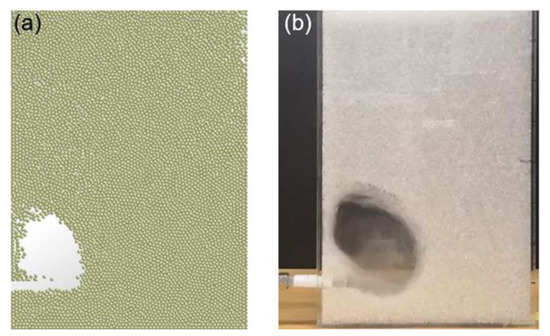
Figure 3.
Void formation obtained in simulation (a) and experiment (b) under the same conditions.
3.2. Dynamic Stability Characteristics of Void
The void morphologies from 2.55 s to 3.55 s in Figure 4a–f show that the morphology changed with time, and the images were obtained per 0.02 s. The particle positions (i.e., blue, red, green, magenta and dark cyan) move along the void boundary with time, which shows the dynamic stable characteristics of the void. To analyze the boundary change of the void quantitatively, we extracted the particle position at the void boundary when t was 2.55 s, 3.15 s and 3.35 s. As shown in Figure 4g, particles at the left and bottom boundaries were located almost in the same position, whereas for those at the top and right boundaries, the distance deviation was 100 mm and 70 mm, void morphology was not static even after the macroscopically stable stage, that is, the void morphology is in a dynamic stable state with time. Therefore, it may be inaccurate to use the transient morphology of the void as the result during the dynamic stable process.
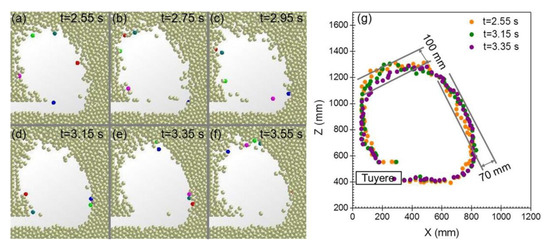
Figure 4.
Void obtained in vinlet = 168 m/s at different times, i.e., (a) t = 2.55 s, (b) t = 2.75 s, (c) t = 2.95 s; (d) t = 3.15 s; (e) t = 3.35 s; (f) t = 3.55 s. (g) Particle position at the void boundary at t = 2.55 s, t = 3.15 s, t = 3.55 s.
3.3. Determination of Dynamically Steady Void Morphology
In this work, a mathematic method was proposed to determine the morphology of a dynamically steady void based on the probabilistic method. Figure 5(a1–a7) show an overlay of the binary image and Ppix,w (e.g., Ppix,w > 0%, Ppix,w > 20%, Ppix,w > 40%, Ppix,w > 50%, Ppix,w > 60%, Ppix,w > 80% and Ppix,w = 100%) at t = 2.95 s. The void area that was obtained by this probabilistic method decreased with an increase in Ppix,w and the void area was smaller than that of binary image when Ppix,w was 100%. We also found that when Ppix,w > 50%, the void area matched the void that was obtained in simulation at t = 2.95 s, as shown in Figure 5(a4).
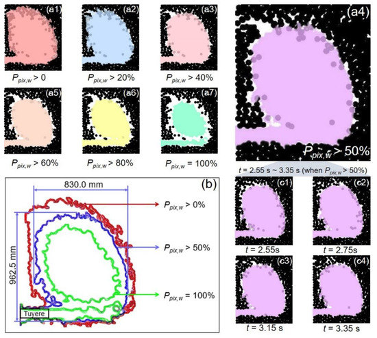
Figure 5.
(a1–a7) In vinlet = 168 m/s, the comparisons between binary image of the void when t = 2.95 s and images for which Ppix,w > 0%, Ppix,w > 20%, Ppix,w > 40%, Ppix,w > 50%, Ppix,w > 60%, Ppix,w > 80% and Ppix,w = 100%, respectively. (b) Boundary and void area size when Ppix,w > 0, Ppix,w > 50% and Ppix,w = 100%. (c1–c4) Comparison of determined void area (Ppix,w > 50%) with DEM results obtained at t = 2.55 s, 2.75 s, 3.15 s and 3.35 s.
To analyze the morphology of the void areas obtained with different Ppix,w (i.e., Ppix,w > 0% (red), Ppix,w > 50% (purple) and Ppix,w = 100% (green)), the probability boundaries were overlaid in Figure 5b. The region outside the boundary of Ppix,w > 0% with only black samples was denoted as a fixed bed, whereas the region inside the boundary of Ppix,w = 100% with only white samples was denoted as an absolute cavity. The area in the middle was denoted as a particle-transition region. The area obtained at Ppix,w > 50% matched the simulated void, therefore, the boundary from Ppix,w > 50% can be defined as the best matching boundary of the void, with a depth and height of 830 mm and 962.5 mm, respectively. Please refer to Appendix C for details.
To verify that the area obtained at Ppix,w > 50% was suitable for determining the void morphology that formed during the dynamic stability process, we compared voids that were obtained in the simulation at t = 2.55 s, 2.75 s, 3.15 s and 3.35 s with the area from Ppix,w > 50%. As shown in Figure 5(c1–c4), the area of Ppix,w > 50% matched the simulation images at different times well, i.e., 42 images. Hence, Ppix,w > 50% can be applied as the well-matched void boundary. Detailed information on the comparisons between the binary images of the void during the dynamic stable process and images at different probabilities is discussed in Appendix C.
3.4. Void Morphology Formed under a Series of Gas Velocities
Previous studies have reported that the void size increases with an increase in gas velocity [15,20,21,34,35]. Various gas velocities were simulated and compared to verify the reliability of our probabilistic method. Figure 6 shows the void morphology formed for five gas velocities, i.e., 168 m/s, 184 m/s, 200 m/s, 216 m/s and 232 m/s, which were determined by using the probabilistic method with Ppix,w > 50%. When the gas velocities were 168 m/s and 184 m/s, the spherical void was formed near the tuyere, with a 200-mm diameter. When the gas velocity increases to 200 m/s, the void height and depth increased to ~450 mm. Therefore, a positive relationship exists between the gas velocity and the void size.
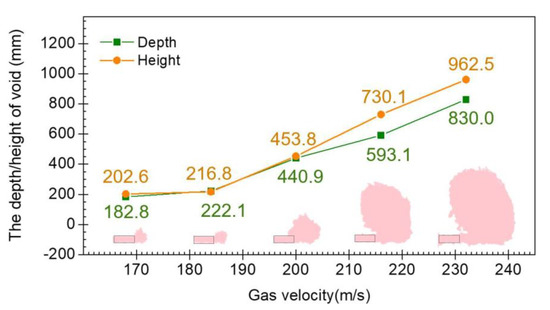
Figure 6.
Void size and shape formed at different gas velocities, determined using the probabilistic method.
Figure 6 shows that the void morphology became a plume-like area when the gas velocity increased (i.e., 216 m/s and 232 m/s), and the void size increased visibly. The void height and depth that formed at 232 m/s increased to 962.5 mm and 830.0 mm, respectively. Because the gas velocity influences the blast kinetic energy, the particle penetration depth in the void changes accordingly. Overall, the void height and depth increase with an increase in gas velocity, which is consistent with the results by Santana et al. [26].
Therefore, the probabilistic method is an effective approach to determine the void morphology. The void boundary that was determined by the probabilistic method was continuous but not smooth, which differed from the previous definition of a void boundary. The method provides an effective strategy to solve the deficiency of DEM results, that is, the transience of the DEM results cannot describe the void change during the dynamic stable process, which is important for theoretical and mathematical modeling of the two-phase gas–solid flow and chemical reaction in and around the void.
4. Conclusions
A 2D two-phase gas–solid flow model in a packed bed was established to simulate the void morphology numerically. Using the CFD–DEM numerical simulation, we discovered that the macroscopically stable voids are dynamically stable because of the particle movement around the boundary. We propose a probabilistic method to determine the void morphology during a dynamic stable process. The boundary at Ppix,w > 50% was selected and defined as the well-matched void boundary. The void morphology that formed at different gas velocities was simulated and compared based on this method to verify the reliability of our probabilistic method. With an increase in gas velocity, the void morphology changes from a small circle around the tuyere to a large, tall and thin ellipse.
Author Contributions
Data curation, Y.L. and S.L.; Funding acquisition, X.Z., Z.J. and D.E.; Supervision, X.Z.; Writing—original draft, Y.L. and S.L.; Writing—review & editing, Y.L., X.Z. and Z.J. All authors have read and agreed to the published version of the manuscript.
Funding
This work was supported by the National Key Research and Development Program of China (2018YFB0605903), the Fundamental Research Funds for the Central Universities (No. FRF–BD–20–09A), and the Key Project of Jiangxi Provincial Research and Development (20192BBHL80016).
Conflicts of Interest
The authors declare no conflict of interest.
Appendix A. Mode Detailed Equations of Drag Force Calculation
Table A1.
Forces and torques acting on particle i.
Table A1.
Forces and torques acting on particle i.
| Forces or Torque | Symbols | Equation |
|---|---|---|
| Normal contact force | Fcn,ij | |
| Normal damping force | Fcd,ij | |
| Tangential contact force | Fct,ij | |
| Tangential damping force | Fdt,ij | |
| Coulomb friction force | Ft,ij | |
| Torque by tangential forces | Mt,ij | |
| Rolling friction torque | Mn,ij |
Table A1 describes the forces and torques acting on particle i, where , ,, , ,, , , , , and , .
, , , , , and e mean the equivalent Young’s modulus, normal amount of overlap, equivalent mass, equivalent radius of the particles, coefficient of restitution, equivalent shear modulus, and tangential stiffness of particles, respectively.
Appendix B. Experiment

Figure A1.
Schematic diagram of the cold physical model. ①—Air compressor; ②—Valve; ③—Rotor flow meter; ④—Cold model; ⑤—Data acquisition system.
Figure A1.
Schematic diagram of the cold physical model. ①—Air compressor; ②—Valve; ③—Rotor flow meter; ④—Cold model; ⑤—Data acquisition system.

Figure A1 shows the experimental facility, the experimental facilities consist of the air compressor, the valve, the rotor flow meter, the cold model and the data acquisition system.
Experimental procedure:
- Connect the experimental equipment;
- Open air compressor and close after checking for air leakage;
- Pour particles into the model for a certain height, and make the surface horizontal;
- Open the air compressor and increase the flow rate to the experimental condition;
- Take photos after the void is stabilized;
- Using software to calculate the void size.
Table A2.
Materials properties and parameters used in the experiment.
Table A2.
Materials properties and parameters used in the experiment.
| Properties | Value | Properties | Value |
|---|---|---|---|
| Length (mm) | 260 | Gas density (kg/m3) | 1.23 |
| Height (mm) | 600 | Gas viscosity (kg/(m·s)) | 1.78 × 10⁻⁵ |
| Thickness (mm) | 17.7 | Gas flow rate (m3/h) | 16 |
| Tuyere diameter (mm) | 10 | Particle materials | PMMA |
| Tuyere depth (mm) | 30 | Particle diameter (mm) | 3–4 |
| Tuyere center height (mm) | 50 | Particle bulk density (kg/m3) | 1000 |
| Packed bed height (mm) | 350 | Particle angle of repose (°) | 35–45 |
Table A2 shows the materials properties and parameters used in the experiment. All these parameters are determined by the similarity principle. Figure A2 shows the experimental result. There is a layer of transition zone at the void boundary.

Figure A2.
The void depth and height in the experiment.
Figure A2.
The void depth and height in the experiment.

The void depth in experiment is 105.1 mm, the void height is 120 mm, the ratio of height and depth is 1.14. The void depth in simulation is 830 mm, the void height is 962.5 mm, the ratio of height and depth is 1.16. The shape of the void in simulation is similar to the experiment, which proves that the mathematical model is accurate.
Appendix C. Probabilistic Statistical Method
The Graythesh function was used to analyze each pixel in the gray images obtained by DEM results. The gray image corresponds to a two-dimensional data matrix. Each element in the matrix represents the gray value of the corresponding pixel, where 0 represents black and 255 represents white. Image binarization can be carried out according to the following formula:
where G(x,y) is the gray value of the pixel, and k is the gray threshold. According to this algorithm, the image was transformed into a binary image and processed.
In the Otsu method, supposing that there are N pixels and L gray levels in the image, the pixel number of gray level i is ni, then the probability distribution is . For the single threshold segmentation, the image is divided into two classes: (C0) and (C1), then the probability of occurrence of C0 and C1 is and , respectively, and the average gray level is μ0 and μ1, respectively. The is the total mean level of the original picture. The between-cluster variance can be determined by,
When the reaches the maximum k, it is defined as the optimal segmentation threshold.

Figure A3.
The comparisons between the binary image of the void when t = 2.55 s, 2.75 s, 2.95 s, 3.15 s, 3.35 s, and 3.55 s and the images of which Ppix,w > 0%, Ppix,w > 20%, Ppix,w > 40%, Ppix,w > 50%, Ppix,w > 60%, Ppix,w > 80% and Ppix,w = 100%, respectively.
Figure A3.
The comparisons between the binary image of the void when t = 2.55 s, 2.75 s, 2.95 s, 3.15 s, 3.35 s, and 3.55 s and the images of which Ppix,w > 0%, Ppix,w > 20%, Ppix,w > 40%, Ppix,w > 50%, Ppix,w > 60%, Ppix,w > 80% and Ppix,w = 100%, respectively.

Figure A3 shows the comparisons between the binary images of the void during the dynamic stability process and the images at different probability. The results show that the probability image with probability ≥ 50% is in good agreement with the void morphology at six different times, which can prove the stability of the void in 2.55–3.55 s. By using the probability method, the morphology of the probability image with the probability of Ppix,w > 50% can be defined as the shape of the void in the dynamic stability process. The void boundary obtained by the probabilistic statistical method is continuous, which solves the shortcomings of the DEM result, i.e., the boundary formed by the discreteness of particles is discrete. The instantaneous character of the DEM result cannot express the dynamic stability of the void. The results of the probabilistic statistical method are in good agreement with the DEM results and the experimental results. This method provides an effective means to study the morphology of voids.
References
- Xu, J.; Yu, S.; Wang, N.; Chen, M.; Shen, Y. Characterization of high-turbulence zone in slowly moving bed slagging coal gasifier by a 3D mathematical model. Powder Technol. 2017, 314, 524–531. [Google Scholar] [CrossRef]
- Wei, G.; Zhang, H.; An, X.; Xiong, B.; Jiang, S. CFD-DEM study on heat transfer characteristics and microstructure of the blast furnace raceway with ellipsoidal particles. Powder Technol. 2019, 346, 350–362. [Google Scholar] [CrossRef]
- Sun, J.; Luo, Z.; Zou, Z. Numerical simulation of raceway phenomena in a COREX melter-gasifier. Powder Technol. 2015, 281, 159–166. [Google Scholar] [CrossRef]
- Flint, P.J.; Burgess, J.M. A fundamental study of raceway size in two dimensions. Metall. Trans. B 1992, 23, 267–283. [Google Scholar] [CrossRef]
- Macdonald, J.F.; Bridgwater, J. Void formation in stationary and moving beds. Chem. Eng. Sci. 1997, 52, 677–691. [Google Scholar] [CrossRef]
- Gupta, G.S.; Litster, J.D.; Rudolph, V.; White, E.T.; Domanti, A. Model Studies of Liquid Flow in the Blast Furnace Lower Zone. ISIJ Int. 1996, 36, 32–39. [Google Scholar] [CrossRef]
- Wagstaff, J.B.; Holman, W.H. Comparison of blast furnace penetration with model studies. Jom 1957, 9, 370–376. [Google Scholar] [CrossRef]
- Szekely, J.; Poveromo, J.J. A mathematical and physical representation of the raceway region in the iron blast furnace. Metall. Mater. Trans. B 1975, 6, 119–130. [Google Scholar] [CrossRef]
- Sarkar, S.; Gupta, G.S.; Kitamura, S.-Y. Prediction of Raceway Shape and Size. ISIJ Int. 2007, 47, 1738–1744. [Google Scholar] [CrossRef][Green Version]
- Rajneesh, S.; Gupta, G.S. Importance of frictional forces on the formation of cavity in a packed bed under cross flow of gas. Powder Technol. 2003, 134, 72–85. [Google Scholar] [CrossRef]
- Gupta, G.S.; Rajneesh, S.; Singh, V.; Sarkar, S.; Rudolph, V.; Litster, J.D. Mechanics of raceway hysteresis in a packed bed. Metall. Mater. Trans. B 2005, 36, 755–764. [Google Scholar] [CrossRef]
- Nogami, H.; Kawai, H.; Yagi, J.-I. Measurement of Three-Dimensional Raceway Structure in Small Scale Cold Model by X-ray Computed Tomography. Tetsu-to-Hagane 2014, 100, 256–261. [Google Scholar] [CrossRef]
- Luo, Z.G.; Sun, Y.; Liu, H.H.; Zou, Z.S. Determination of raceway boundary with particle velocity contour. Chin. J. Process. Eng. 2009, 9, 228–232. [Google Scholar]
- Di, Z.; Luo, Z.; Han, Y.; Zou, Z.; Li, L. Fractal Study on Raceway Boundary. J. Iron Steel Res. Int. 2011, 18, 16–19. [Google Scholar] [CrossRef]
- Lu, Y.; Jiang, Z.; Zhang, X.; Liu, S.; Wang, J.; Zhang, X. Determination of void boundary in a packed bed by laser attenuation measurement. Particuology 2020, 51, 72–79. [Google Scholar] [CrossRef]
- Rangarajan, D.; Shiozawa, T.; Shen, Y.; Curtis, J.S.; Yu, A. Influence of Operating Parameters on Raceway Properties in a Model Blast Furnace Using a Two-Fluid Model. Ind. Eng. Chem. Res. 2014, 53, 4983–4990. [Google Scholar] [CrossRef]
- Kawaguchi, T.; Tanaka, T.; Tsuji, Y. Numerical simulation of two-dimensional fluidized beds using the discrete element method (comparison between the two- and three-dimensional models). Powder Technol. 1998, 96, 129–138. [Google Scholar] [CrossRef]
- Tsuji, Y.; Kawaguchi, T.; Tanaka, T. Discrete particle simulation of two-dimensional fluidized bed. Powder Technol. 1993, 77, 79–87. [Google Scholar] [CrossRef]
- Tsuji, Y.; Tanaka, T.; Ishida, T. Lagrangian numerical simulation of plug flow of cohesionless particles in a horizontal pipe. Powder Technol. 1992, 71, 239–250. [Google Scholar] [CrossRef]
- Xu, B.H.; Yu, A.B.; Chew, S.J.; Zulli, P. Numerical simulation of the gas-solid flow in a bed with lateral gas blasting. Powder Technol. 2000, 109, 13–26. [Google Scholar] [CrossRef]
- Miao, Z.; Zhou, Z.; Yu, A.; Shen, Y.J.P.T. CFD-DEM simulation of raceway formation in an ironmaking blast furnace. Powder Technol. 2017, 314, 542–549. [Google Scholar] [CrossRef]
- Guo, J.; Cheng, S.; Zhao, H.; Pan, H.; Du, P.; Teng, Z. A Mechanism Model for Raceway Formation and Variation in a Blast Furnace. Metall. Mater. Trans. Part B. 2013, 44, 487–494. [Google Scholar] [CrossRef]
- Umekage, T.; Yuu, S.; Kadowaki, M.J.I.I. Numerical Simulation of Blast Furnace Raceway Depth and Height, and Effect of Wall Cohesive Matter on Gas and Coke Particle Flows. ISIJ Int. 2005, 45, 1416–1425. [Google Scholar] [CrossRef]
- Santana, E.R.; Pozzetti, G.; Peters, B. Application of a dual-grid multiscale CFD-DEM coupling method to model the raceway dynamics in packed bed reactors. Chem. Eng. Sci. 2019, 205, 46–57. [Google Scholar] [CrossRef]
- Cundall, P.A.; Strack, O.D.L. Discussion: A discrete numerical model for granular assemblies. Geotechnique 1980, 30, 331–336. [Google Scholar] [CrossRef]
- Mindlin, R.D.; Deresiewicz, H. Elastic Spheres in Contact under Varying Oblique Forces. J. Appl. Mech-T ASME 1953, 20, 327–344. [Google Scholar]
- Dong, Z.; Wang, J.; Liu, J.; She, X.; Xue, Q.; Lin, L. Gas-Solid Flow and Injected Gas Distribution in OBF Analyzed by DEM-CFD. In CFD Modeling and Simulation in Materials Processing 2016; Springer LLC: Synergy Flavors, OH, USA, 2016; pp. 229–237. [Google Scholar]
- Ergun, S. Fluid Flow through Packed Column. Chem. Eng. Prog. 1952, 48, 89–94. [Google Scholar]
- Wen, C.Y.; Yu, Y.H. Mechanics of Fluidization. Chem. Eng. Prog. Symp. Ser. 1966, 62, 100–111. [Google Scholar]
- Zhou, Z.; Zhu, H.; Wright, B.; Yu, A.; Zulli, P. Gas–solid flow in an ironmaking blast furnace-II: Discrete particle simulation. Powder Technol. 2011, 208, 72–85. [Google Scholar] [CrossRef]
- Otsu, N. A Threshold Selection Method from Gray-Level Histograms. IEEE Trans. Syst. Man Cybern. 1979, 9, 62–66. [Google Scholar] [CrossRef]
- Pashchenko, D. Flow dynamic in a packed bed filled with Ni-Al2O3 porous catalyst: Experimental and numerical approach. AIChE 2019, 65, e16558. [Google Scholar] [CrossRef]
- Pashchenko, D.; Karpilov, I.; Mustafin, R. Numerical calculation with experimental validation of pressure drop in a fixed-bed reactor filled with the porous elements. AIChE 2020, 66, e16937. [Google Scholar] [CrossRef]
- Hilton, J.E.; Cleary, P.W. Raceway formation in laterally gas-driven particle beds. Chem. Eng. Sci. 2012, 80, 306–316. [Google Scholar] [CrossRef]
- Cui, J.; Hou, Q.; Shen, Y. CFD-DEM study of coke combustion in the raceway cavity of an ironmaking blast furnace. Powder Technol. 2020, 362, 539–549. [Google Scholar] [CrossRef]


© 2020 by the authors. Licensee MDPI, Basel, Switzerland. This article is an open access article distributed under the terms and conditions of the Creative Commons Attribution (CC BY) license (http://creativecommons.org/licenses/by/4.0/).