MMC-Based PV Single-Phase System with Distributed MPPT

Abstract

The presence and evolution of static power converters in electric grids are growing on a daily basis. Starting from the most used voltage source converter (VSC), passing through the use of multilevel converters, the most recent configuration is the so-called modular multilevel converter (MMC). Because of its intrinsic advantages, it is used not only in high-voltage systems but also in low- and medium-voltage ones to interface renewable energy sources such as photovoltaic (PV) panels. Several configurations and maximum power point tracker (MPPT) algorithms have been proposed and analyzed for MMC-PV-based systems. However, when using distributed MPPTs, partial shading conditions cause a problem. The PV panel can be directly connected to the MMC using its dc link or submodule. Based on this configuration, this paper proposes a novel control strategy that tracks both the ac grid current and ac circulating current for a single-phase low-voltage system to obtain the maximum power under any irradiance condition. The effectiveness of the proposed control strategy is demonstrated through time-domain simulation results.

1. Introduction

Static power converters are one of the most interesting and promising technologies still under evolution. Their uses are manifold, and their presence in electric networks is growing. In fact, they can be used as electrical drives, active filters, interfaces for joining different electric grids, connection devices for energy storage devices, such as batteries and supercapacitors, and renewable energy sources, such as photovoltaic (PV) panels and wind turbines. The latter are spreading in the entire electric network (high-, medium-, and low-voltage systems). Moreover, they are used to form the well-known micro-grids, which can work either in the island mode or grid-connected mode simply through the use of power converters.

One of the most employed power converters is the voltage source converter (VSC). It is typically composed of insulated-gain-bipolar-transistors (IGBTs), through which two different grids (ac/dc) can be connected to each other. Two- or three-level VSCs are usually employed for low- and medium-voltage systems. On the other hand, in high-voltage systems, because of the limited maximum rated voltage of IGBTs, the use of a traditional multilevel VSC becomes complicated. To overcome this issue, one solution is to use more IGBTs in series to reconstruct the single switches composing the VSC. However, this makes the device more complex and much more expensive with respect to the intrinsic advantages of such a configuration. In recent years, modular multilevel converters (MMCs) represent a novel technology able to overcome the issues related to a high-voltage system while simultaneously presenting other intrinsic advantages. MMCs present a reduced harmonic content, modularity, and more control degrees of freedom. Although MMCs are suitable for high-voltage systems, their other intrinsic advantages can make them suitable for other applications in both medium- and low-voltage systems. In particular, PV panels are usually interfaced with the electric network through voltage source inverters (VSIs) and dc/dc boost converters [1]. The latter are usually employed to extract the maximum power using one of the maximum power point tracking (MPPT) algorithms. In most cases, numerous PV cells are connected in series and parallel to each other to form the PV modules. Several modules can be connected in series to form a string. Different strings can then be connected in parallel to form an array. In the centralized MPPT (CMPPT) configuration, the whole array is usually connected to the ac grid through a single VSI with or without a dc/dc converter and/or a galvanic transformer [2,3,4]. Although this kind of configuration is quite simple, it has a large power loss in the case of partial shading. Indeed, the MPPs of PV modules have different voltage and current values when differently radiated. For this reason, it is not possible, with a single tracker, to make each PV panel work at its MPP [5,6]. In general, the different panels in one PV string could lead to the presence of more than one local maximum in the power–voltage characteristic curve of the equivalent series PV module. This could be a problem for the CMPPT algorithm [7]. In [8,9,10,11,12,13,14], the authors assessed several strategies to find the global maximum power point of that curve. In [15], the authors proposed to change the electrical connections of the PV panels to maximize the configuration under shading conditions. The main drawback of this method is the need for several switches. Another strategy to solve this issue is the use of a distributed MPPT (DMPPT). In the literature, it is possible to find several kinds of DMPPTs. Nevertheless, two main families can be recognized. The first one is the DMPPT at the string level, in which each string of the array is controlled separately to allow each of them to reach its own maximum power point. It is possible to use as many VSIs as strings or only one centralized VSI and a dc/dc converter for each PV string [16,17]. The problem of the partial shading of modules of the same string is still present, and the presence of bypass diodes brings to zero the power produced by the shaded modules. The second family is the DMPPT at the module level. In this way, each PV module is separately controlled by the acting MPPT for each module. This family includes module-integrated parallel inverters (also called PV micro-inverters) [18], module-integrated parallel converters [19,20], module-integrated series converters [21,22], and module-integrated differential power processors [23]. In this way, under any shading condition, each PV module can extract its maximum power. On the other hand, the high number of converters (VSI and or dc/dc converters) yields a very expensive solution.

In recent years, the use of the MMC for PV interfacing has started to be analyzed. The authors in [24] used the MMC to interface PV panels with the grid. In this case, the PV panels were connected to the dc side of the MMC, not allowing the implementation of a DMPPT. A very interesting improvement was made in [25,26], where the authors connected each PV module to each submodule (SM) of the MMC through a boost converter. This method was similar to the one proposed in [18] with several micro-VSIs, and it can be considered to be a DMPPT at the module level solution. However, the high number of boost converters prevents this solution from being optimal. Instead, in [27], a novel and interesting idea was to connect each PV module directly to the capacitor of each SM of the MMC. Therefore, the system is much less expensive but more difficult to control. In fact, in order to extract the maximum power from each PV module, in the case of partial shading, each voltage of each SM capacitor should be controlled at the MPP of the related PV module. This solution presents all the advantages of the structure in which each PV panel is controlled separately, as in [18], with neither the problem of the multi-local power points of the PV strings nor the high number of other converters. Furthermore, all the advantages of the MMC can be used instead of the classical VSI. Nevertheless, in the solution proposed in [27], tests were performed using an MMC structure with only two levels per arm. Moreover, they used one supplemental redundancy module per arm to adjust the dc voltage in the case of shading. Finally, their control strategy fixed the dc voltage of the MMC to a given reference value. In every case, the structure of the converters could be designed for a general number of phases. Although the three-phase structure is the most common, even single-phase and multi-phase structures (with more than three) are used. Focusing on the MMCs, while the three-phase and multi-phase configurations do not need a real dc link, the single-phase MMC, in order to provide the current return path, needs a real dc link with the middle-point accessible [28,29].

In the present work, a structure similar to the one proposed in [27] was proposed and tested, using different simulations. The main contribution of the present work is a method to control the MMC to avoid the use of redundancy modules and directly generate the dc voltage reference using the MPPT algorithm of each PV module. Moreover, the dc voltage reference is not kept constant but depends on the shading conditions. Of course, the dc voltage value is in a working range suitable for producing the required ac voltage. Therefore, the PV panels have to be opportunely sized based on both the number of MMC levels and grid characteristics.

Although most of the connections are performed through three-phase systems, nevertheless, in low-voltage electric networks, even single-phase appliances can be of interest. Moreover, this study can be used as the basis for a future extension in three-phase systems. For this reason, in this work, an MMC structure was investigated for a low-voltage single-phase system with a rated power of 6 kW. This meant that, unlike the structure proposed in [27], in which a three-phase MMC was employed, here a single-phase MMC composed of only two arms and a real dc link with the central point accessible was used.

2. Converter Topology

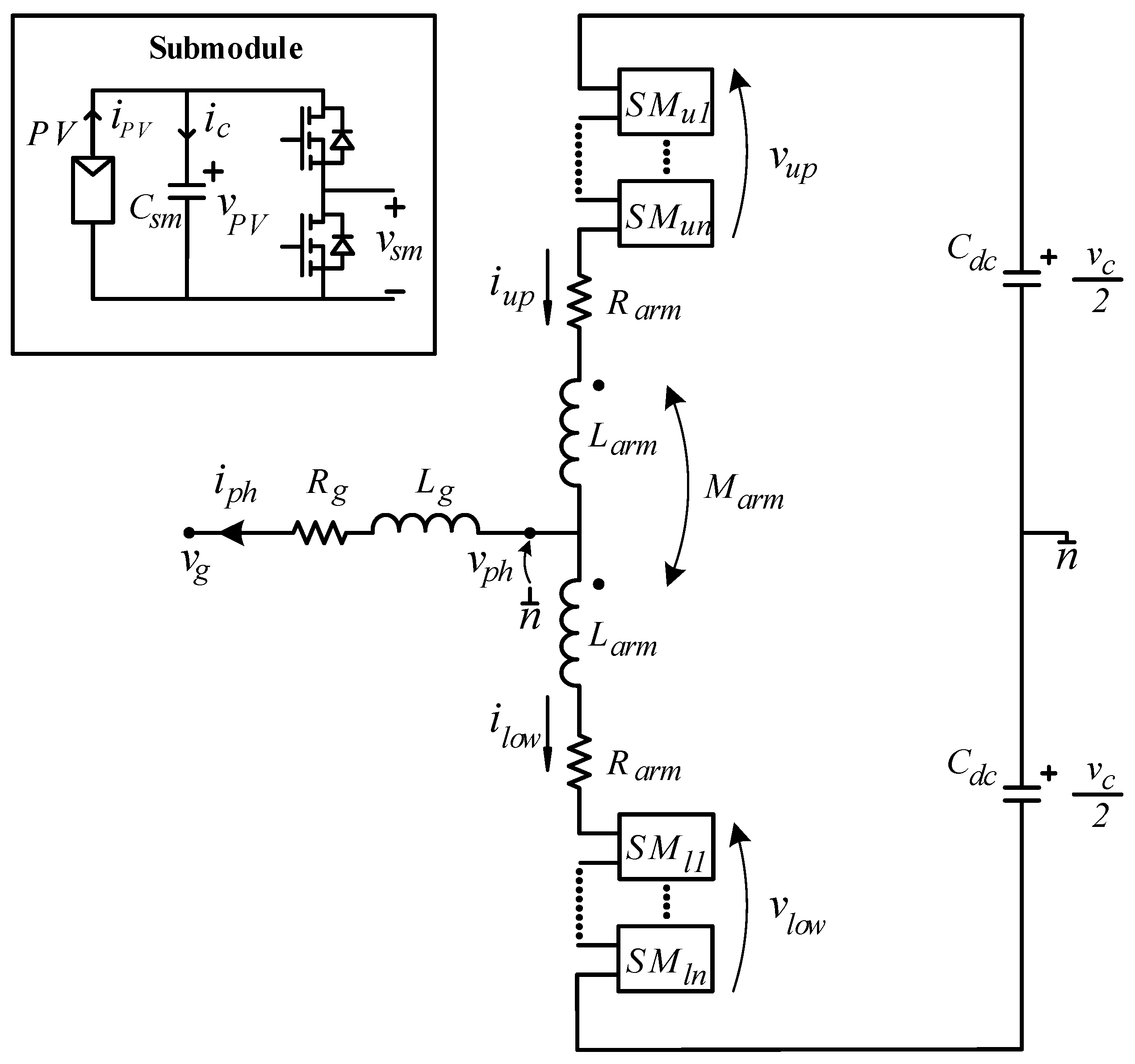
Figure 1 shows the circuit configuration of the proposed single-phase MMC. It is composed of two arms, referred to as the upper and lower arms, whose mid-point is connected to the grid voltage through its resistance R_g and inductance L_g. Each arm of the MMC is composed of a series arrangement of SMs whose switching is coordinated to generate a quasi-sinusoidal output voltage. Moreover, a single coupled arm inductor is used in order to obtain a weight reduction and less influence on the output voltage. Finally, the dc side of the MMC is composed of the two capacitors, C_dc, needed to create the central point for the neutral connection of the grid.

Considering Figure 1, according to Kirchoff’s voltage law, the following expressions can be derived:

$$\{\begin{array}{l}{v}_{ph}=\frac{v_c}{2}-v_{up}-R_{arm}{i}_{up}-L_{arm}\frac{d{i}_{up}}{dt}-M_{arm}\frac{d{i}_{low}}{dt}\\ v_{ph}=-\frac{v_c}{2}+v_{low}+R_{arm}{i}_{low}+L_{arm}\frac{d{i}_{low}}{dt}+M_{arm}\frac{d{i}_{up}}{dt}\end{array}$$

(1)

where v_ph is the output phase voltage of the MMC; v_up and v_low are the voltages applied by the upper and lower arms, respectively; v_c is the voltage of the dc bus; R_arm is the arm resistance; L_arm is the arm inductance, and M_arm is the mutual coupling of the arm inductances. Finally, i_up and i_low are the upper and lower arm currents, respectively. Let us define grid current i_ph and circulating current i_circ as follows:

$$\{\begin{array}{l}{i}_{ph}=i_{up}-i_{low}\\ i_{circ}=\frac{i_{up}+i_{low}}{2}\end{array}$$

(2)

Furthermore, we can define the circulating voltage as follows:

$$v_{circ}=v_{low}+v_{up}$$

Therefore, according to (1) and (2), the output phase voltage can be expressed as follows:

$$v_{ph}=\frac{v_{low}-v_{up}}{2}-\frac{R_{arm}}{2}{i}_{ph}-\frac{L_{arm}}{2}\frac{d{i}_{ph}}{dt}+\frac{M_{arm}}{2}\frac{d{i}_{ph}}{dt}$$

(3)

and the output circulating voltage is

$$v_{circ}=-\left(2R_{arm}{i}_{circ}+2L_{arm}\frac{d{i}_{circ}}{dt}+2M_{arm}\frac{d{i}_{circ}}{dt}\right)+v_c$$

(4)

The voltage of the dc bus is supported by the two C_dc capacitors. Thus, it can be obtained as follows:

$$v_c(t)=-\frac{2}{C_{dc}}{\displaystyle \underset{0}{\overset{t}{\int }}{i}_{circ}d\tau }+v_c(0)$$

(5)

where v_c(0) is the initial voltage value of the dc bus.

Under normal working conditions, the output phase voltage contains only the fundamental ac component, while the circulating voltage has to contain a dc component as well. In fact, the MMC needs an opportune dc voltage to work correctly. The latter is the dc voltage that charges the two C_dc capacitors to the dc voltage. This means that under a steady state condition, the dc component of the circulating voltage does not produce any dc component in the circulating current. Thus, the integral term in (5) will have a zero average value. On the other hand, during transients, the circulating current contains a dc component that charges or discharges the C_dc capacitors.

Moreover, looking at (3), by using coupled arm inductors with a unitary coupling coefficient, the output phase voltage, v_ph, does not depend on the arm inductance but only on the difference between the voltages applied by the upper and lower arms. In light of the above, the output phase voltage (with only the ac component) is related to the powers exchanged (active and reactive) with the grid, while the ac component of the circulating voltage is related to the portioning of those powers between the two arms. In fact, in a case where the two arms had the same solar irradiances, the total power exchanged with the grid would be equally divided between the two arms themselves. Therefore, the circulating current would be nil. On the other hand, if the available powers in the two arms were different from each other, the circulating current would no longer be nil. This is a crucial aspect for our controller because to extract the maximum power from each PV module under any irradiance condition, it should provide an opportune value for the circulating current.

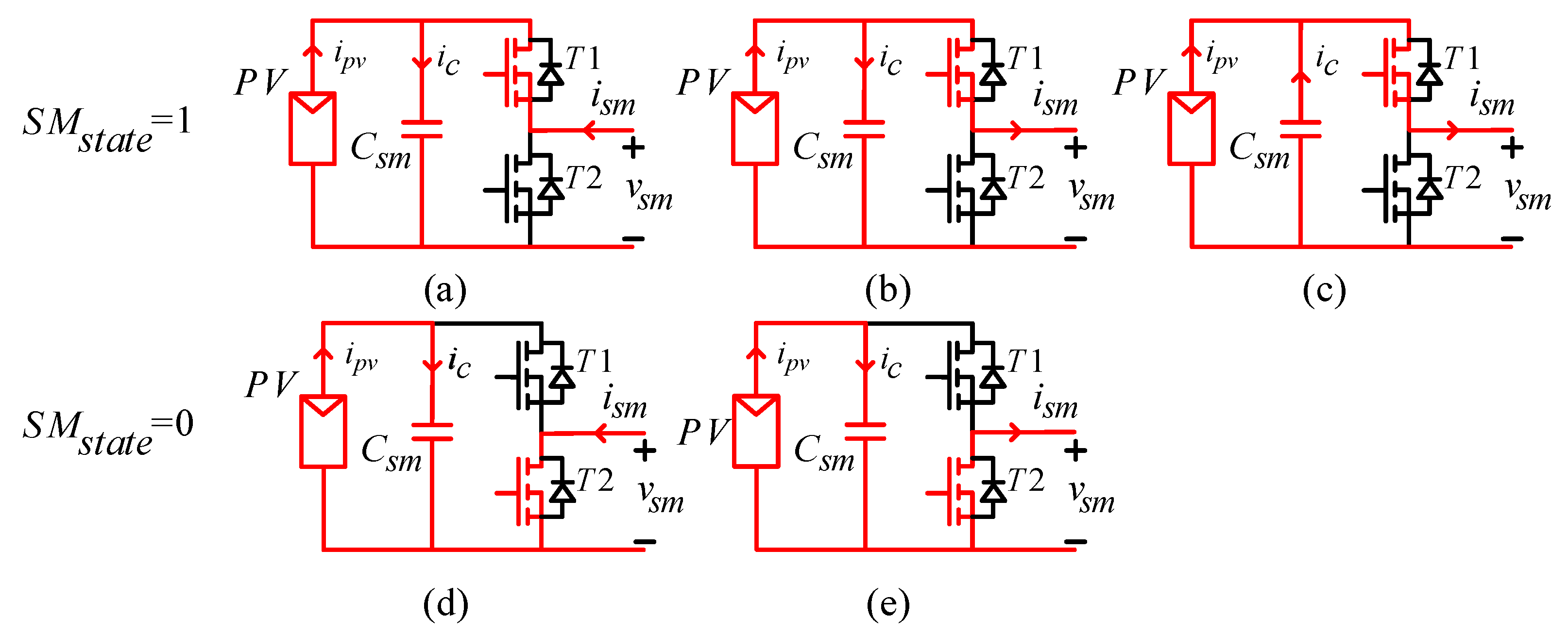
The two arms are composed of a series of a certain number of SMs. Each SM is composed of a half-bridge converter connected to cell capacitor C_sm and a PV module. Considering that the two switch states are always complementary to each other, the possible SM states are as follows:

• SM_state = 1
  When the SM is in state 1, whether arm current i_sm is positive or negative, switch T1 is in the conduction mode. Under the condition shown in Figure 2a, the current that flows through the capacitor, the sum of i_pv and i_sm, charges it. If the arm current is negative and less than i_pv in magnitude, the current that flows through the capacitor will charge it (Figure 2b). Instead, if the arm current is negative but higher than i_pv in magnitude, the capacitor will discharge (Figure 2c).
• SM_state = 0
  When the SM is in state 0, whether arm current i_sm is positive or negative, switch T2 is in the conduction mode. In both cases, only the PV current will flow through the capacitor charging it.

3. Converter Sizing

The circuit parameters can be designed starting from grid voltage v_g and the power ratings. The minimum operational dc voltage, taking into account that the converter should provide active and reactive power, is defined as follows:

$$v_{dc\_min}=2k{v}_{g\_peak}$$

(6)

where k is a correction factor needed for power regulation, and v_{g_peak} is the peak of the rated grid voltage.

Then, the number of SMs is defined according to different requirements such as the total harmonic distortion, converter power losses, and power and voltage ratings of the semiconductor devices.

Moreover, the PV modules embedded in each SM of the MMC are composed of the series and parallel connections of several PV sub-modules. The number of series PV sub-modules can be derived as follows:

$$n_{pv\_series}=\frac{v_{dc\_min}}{n_{sm}{V}_{mppt\_min}}$$

(7)

where n_sm is the number of sub-modules and V_{mppt_min} is the minimum optimal operative PV voltage determined at the minimum irradiance at which the system should work. In this way, the proper operation of the system at irradiances different from the maximum one is guaranteed.

Then, in order to reach the desired power rating, the number of parallel PV sub-modules is defined as follows:

$$n_{pv\_parallel}=\frac{P_{rated}}{n_{arm}{n}_{sm}{n}_{pv\_series}{P}_{pv}}$$

(8)

where P_rated is the rated plant power, n_arm is the number of arms (i.e., two in the single-phase MMC), and P_pv is the rated power of a single PV sub-module.

4. Proposed Control Strategy

The proposed control strategy is designed in order to generate the following voltage references for the upper and lower arms:

$$\{\begin{array}{l}{v}_{up}^{*}=-v_{ph}^{*}+\frac{v_{circ}^{*}}{2}\\ v_{low}^{*}=v_{ph}^{*}+\frac{v_{circ}^{*}}{2}\end{array}$$

(9)

where $v_{ph}^{*}$ is the output phase voltage reference that contains only the ac component, and $v_{circ}^{*}$ is the circulated voltage reference defined as follows:

$$v_{circ}^{*}=v_{circ,ac}^{*}+V_{dc}^{*}.$$

(10)

As previously stated, the dc component of the circulating voltage, V_dc, is the dc voltage of the MMC, while the ac component is controlled to extract the maximum power from each arm under any irradiance conditions.

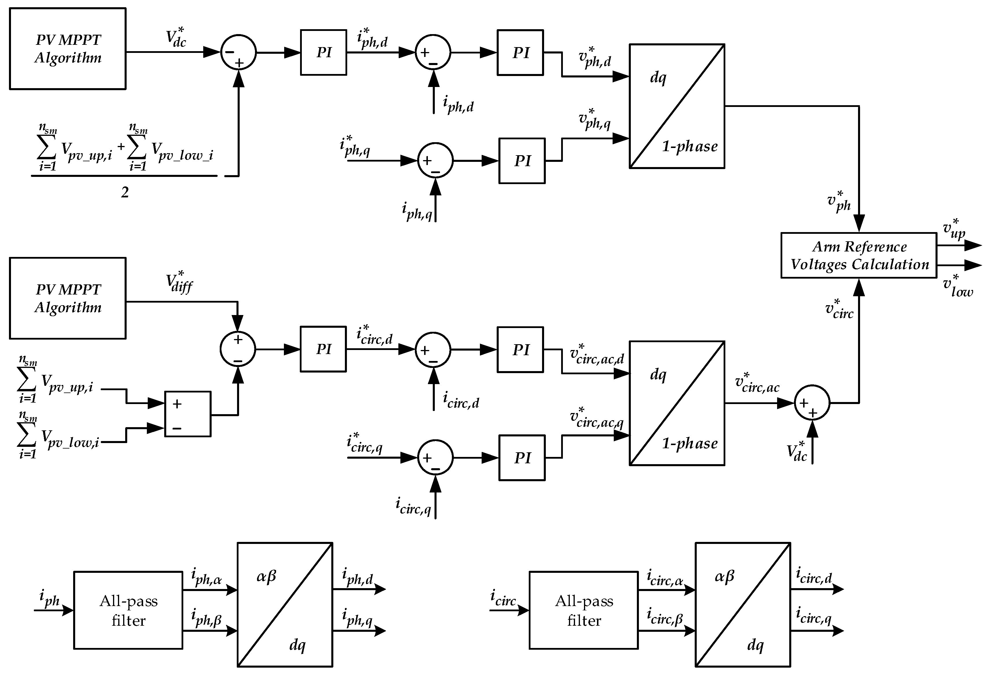
Figure 3 shows the scheme of the proposed control strategy. This can be divided into three main controllers: the MPPT control system, power management system, and modulation technique. The MPPT control system defines the optimal voltage references of all the PV modules. These reference signals, through the power management system, define the reference dc voltage, $V_{dc}^{*}$, and the reference voltages of the SM capacitors, i.e., the voltages of the PV modules, V_{pv_up,i} and V_{pv_low,i}, in order to extract the maximum power at a given solar irradiance. Therefore, this controller gives the related output phase and circulating voltage references, which according to (9), generate the output upper and lower arm voltage references. Finally, these references are synthesized through the MMC by implementing the phase disposition pulse width modulation technique (PD-PWM) [30]. Its operating principle is to compare the reference with multiple carriers placed at different levels having the same amplitude, frequency, and phase angle.

4.1. MPPT Control System

The MPPT control system is a crucial part of the PV system. Indeed, its aim is to define both the total dc voltage, V^*_dc, at which the MMC should operate and the voltages of each PV module, V_{pv_up,i} and V_{pv_low,i}, to obtain their maximum power under a given solar irradiance.

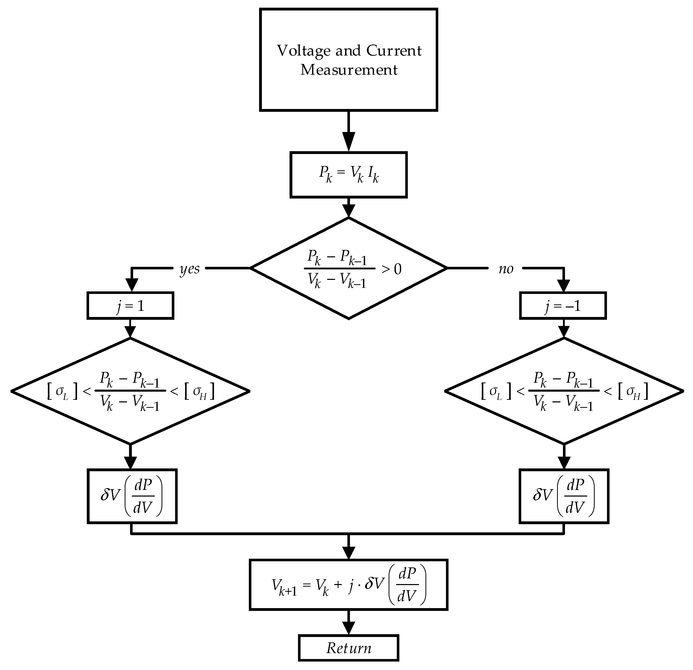
Several methods to estimate the maximum power point have been proposed in the literature, including the hill climbing, perturb and observe (P&O), incremental conductance, fractional short circuit current, fractional open circuit voltage, fuzzy logic, neural network, and other methods reviewed in [31]. In the present study, the P&O method was selected because it is a more straightforward and diffused method that induces a perturbation in the operating voltage of the PV system. In particular, an adaptive P&O algorithm was implemented. The main difference with the traditional P&O algorithm was the fact that the perturbation applied was not a fixed value but changed with the dP/dV ratio. Defining certain thresholds, a larger dP/dV ratio led to a greater perturbation value being applied and vice versa. In this way, a good dynamic performance and stability at a steady state were ensured.

In the proposed control strategy, the MPPT algorithm (Figure 4) is applied to each PV module, and it can be summarized in the following two steps. (i) The currents, i_{pv_up,i} and i_{pv_low,i}, and voltages, V_{pv_up,i} and V_{pv_low,i}, of each PV module of the two arms, are measured, and thus, the power produced is obtained; (ii) A positive or negative voltage perturbation is applied until the algorithm reaches the maximum power point, which is when the ratio of dP/dV is ideally equal to 0. The absolute value of the perturbation, δV, applied depends on the distance from the real maximum power point according to different thresholds implemented in the controller:

$$\left[{\sigma }_L\right]<\frac{P_k-P_{k-1}}{V_k-V_{k-1}}<\left[{\sigma }_H\right];P_k=V_k{I}_k$$

where $\left[{\sigma }_L\right]$ and $\left[{\sigma }_H\right]$ are vectors composed of N thresholds as follows:

$$\begin{array}{l}\left[{\sigma }_L\right]=[0{\sigma }_1{\sigma }_2\dots {\sigma }_{N-1}]\\ \left[{\sigma }_H\right]=[{\sigma }_1{\sigma }_2\dots {\sigma }_{N-1}\infty ].\end{array}$$

V_k, I_k, and P_k are, respectively, the voltage, current and power of the PV modules at time instant k. The outputs of the MPPT controller are all the optimal voltages of each PV module of the two arms, V_{pv_mppt_up,i} and V_{pv_mppt_low,i}.

4.2. Power Management System

Because a single-phase system was analyzed, we decided to use one of the orthogonal signal techniques [32,33] and dq transformations, which made it possible to implement the control system in a synchronous reference frame [34]. The orthogonal signal generation techniques needed to create a fictitious imaginary component of the real electric quantity. We chose to use an all-pass filter that could easily approximate the Hilbert transformation [32]. The latter, from a mathematical point of view, can provide a signal that in the Fourier domain has the same harmonic content of the transformed signal with all the components shifted by −90°. The all-pass filter was synthesized by the following Laplace function:

$$H(s)=\frac{{\omega }_f-s}{{\omega }_f+s}$$

(11)

where ω_f is the fundamental angular frequency, and s is the Laplace variable.

The αβ coordinates of the system can be obtained using the Hilbert transformation. In particular, the β component turned out to lag by 90° with respect to the fundamental one. Then, the dq transformation from a rotating to stationary frame is given by the following:

$$\left[\begin{array}{l}{x}_d(t)\\ x_q(t)\end{array}\right]=\left[\begin{array}{cc}cos(\theta )& sin(\theta )\\ -sin(\theta )& cos(\theta )\end{array}\right]\left[\begin{array}{l}{x}_{\alpha }(t)\\ x_{\beta }(t)\end{array}\right]$$

(12)

where θ represents the electrical voltage angle.

In order to ensure the maximum power produced by the PV systems, a control system oriented on the grid voltage was used, as shown in Figure 3. This controller generated the output phase voltage and circulating voltage references as functions of the voltage references provided by the MPPT controller.

The power management system could be subdivided into two subsystems: the grid and circulating controllers. Each of these two controllers was composed of two inner PI regulators and one outer PI regulator.

4.2.1. Grid Controller

The outer control loop of the grid controller tracked the dc bus voltage to the reference one. The latter was defined according to the mean value of the MPPT reference voltages as in the following equation:

$$V_{dc}^{*}=\frac{{\displaystyle \sum _{i=1}^{n_{sm}}{V}_{pv\_mppt\_up,i}+}{\displaystyle \sum _{i=1}^{n_{sm}}{V}_{pv\_mppt\_low,i}}}{2}.$$

(13)

It is worth noting that, unlike the control proposed in [27], in the present work, the dc voltage reference was not fixed and could change as a function of the irradiance. Therefore, from the outer PI regulator, the direct component of the current reference, $i_{ph,d}^{*}$, proportional to the maximum active achievable power, was obtained. Instead, the quadrature component of current reference $i_{ph,q}^{*}$ made it possible to regulate the desired reactive power. For the sake of simplicity, its reference was assumed to be equal to 0 in order to exchange the rated active power at a unitary power factor.

The inner control loop regulated the direct and quadrature components of the grid current and reference voltages $v_{ph,d}^{*}$ and $v_{ph,q}^{*}$ were generated by means of two inner PI controllers. Moreover, the feed-forward terms could be used to improve the dynamic response. The inverse dq transform yielded the output grid voltage reference, $v_{ph}^{*}$, which corresponded to the α component.

4.2.2. Circulating Controller

The direct component of the circulating current reference, $i_{circ,d}^{*}$, similar to that of the grid current reference, was generated through a PI controller that tracked the difference between the upper and lower optimal voltages as follows:

$$V_{diff}^{*}={\displaystyle \sum _{i=1}^{n_{sm}}{V}_{pv\_mppt\_up,i}-}{\displaystyle \sum _{i=1}^{n_{sm}}{V}_{pv\_mppt\_low,i}}.$$

(14)

This controller was implemented in order to guarantee that each arm could operate at its own optimal average voltage providing its maximum active power. Therefore, the direct component of the circulating current was zero only if the two arms had the same average irradiance. Otherwise, if the two arms had different average irradiances, this circulating current component had to be different from zero to allow a power imbalance between the two arms. The quadrature component of reference circulating current $i_{circ,q}^{*}$ was set equal to 0. In this way, the reactive power exchanged by the two arms was proportional to the direct component. In fact, the voltages of the two arms were not in phase with the grid voltage. This was obvious because the active power was exchanged with the grid through an inductive line. This displacement was the load angle. Therefore, even if the reactive power exchanged with the grid was zero (unity power factor), the reactive power needed to charge the inductors was given by the MMC.

The inner control loop regulated the direct and quadrature components of the circulating current and, by means of two inner PI controllers, reference voltages $v_{circ,ac,d}^{*}$ and $v_{circ,ac,q}^{*}$ were generated. Moreover, the feed-forward terms could be used to improve the dynamic response. The inverse dq transform yielded the output circulating voltage reference, $v_{circ,ac}^{*}$, which corresponded to the α component.

Finally, the upper and lower arm voltage references could be calculated according to (9) and (10).

It is worth noting that each sum of (13) and (14) represents the maximum voltage that can be obtained by each arm when all the SMs are activated (maximum arm voltage). According to (9) and (10), in addition to the ac components, each arm has to be able to synthesize half of the dc voltage reference given by (13). In case of equal irradiance conditions between the two arms, the dc voltage reference coincides with the maximum arm voltages. In this way, the ac voltage components can be synthesized using all the SM voltage levels of the arms. Conversely, in case of different irradiance conditions between them, the dc voltage reference deviates from the two maximum arm voltages according to (14), thus, the ac voltage components can be synthesized only using a subpart of the SM voltage levels of the arms. Since the irradiance conditions slightly affect the MPPT voltages, taking it into account in the sizing procedure through the correction factor of (6), it is possible to make the MMC work even for significant irradiance differences between the arms.

4.3. Submodule Sorting

To follow the maximum power peak point and exploit the power produced by the PV systems, the following balance algorithm was defined:

• If the arm current is positive, it charges the capacitors; the SM with the farthest capacitor voltage from its theoretical optimal voltage and on the left side of the MPP is activated first to produce the desired output voltage.
• If the arm current is negative, it discharges the capacitors; the SM with the farthest capacitor voltage from its theoretical optimal voltage and on the right side of the MPP is activated first to produce the desired output voltage.

Therefore, with the proposed sorting algorithm, each PV input voltage is compared with its own theoretical optimal voltage and, in this way, it can work continuously around its maximum power point.

5. Results

The effectiveness and powerfulness of the proposed DMPPT at the module level were demonstrated through simulations performed in Matlab Simulink^®. As reported in the previous section, the ac circulating current component was controlled to guarantee the management of the power mismatch between the two arms of the MMC. Moreover, the submodule sorting based on the DMPPT made each PV module work at its own maximum power point. A comparison of the proposed DMPPT controller with the CMPPT one was performed. The latter was simply obtained by using the traditional submodule sorting [35] (instead of the one proposed in Section 4.3) and keeping the average voltage arms equal. This meant that (14) was equal to zero. The traditional SM sorting algorithm ordered them based on the increasing/decreasing values of the voltages of the SM capacitors, while the zeroing of (14) allowed the whole system to work at the maximum point of the equivalent PV array. Moreover, two different solar irradiation scenarios were considered for the comparison. The main parameters of the used MMC-PV system are summarized in

Table 1. Main MMC-PV system parameters.

Parameters	Value	Units
Rated plant power Prated	6	kW
Rated grid voltage (rms) vg	230	V
Grid resistance Rg	140	mΩ
Grid inductance Lg	3.9	mH
Arm resistance Rarm	1	mΩ
Arm inductance Larm	1	mH
Mutual arm inductance Marm	0.99	mH
SM capacitor Csm	10	mF
dc bus capacitor Cdc	2	mF
Correction factor for power regulation k	1.1	-
Minimum operational dc voltage vdc,min	715.6	V
Number of SMs per arm nsm	10	-

.

Moreover, each PV power module, P_{pv_i}, was modeled as follows [36]:

$$P_{pv\_i}=(2.06\cdot G_i-1.58\times {10}^{-8}-1.58\times {10}^{-8}\cdot e^{\left(0.72\cdot V_{pv\_i}/n_{pv\_series}\right)})\cdot n_{pv\_parallel}\cdot V_{pv\_i}$$

(15)

where G_i and V_{pv_i} are the solar irradiation and voltage of the i-th PV module, respectively. The parameters of the PV modules are listed in

Table 2. PV module parameters.

Parameters	Value	Units
Rated power Ppv	42.53	W
Minimum operative irradiance Gmin	200	W/m2
Minimum optimal operative PV voltage Vmppt,min	19.9	V
Number of series PV sub-module npv_series	2	-
Number of parallel PV sub-module npv_parallel	4	-

. For the sake of simplicity, all the simulations were performed considering the PV temperature fixed at 25 °C. For this reason, the (15) contains the constant parameters calculated for that temperature. This is because a change in the temperature leads to a different maximum power point without changing the shape of the PV characteristic.

5.1. Scenario 1. Partial Shading Conditions in One Arm

In this case, a partial shading condition between the two arms was analyzed. Initially, both the arms were irradiated at the maximum value, i.e., 1000 W/m². Then, after 7 s, the solar irradiance fell to 300 W/m² for all the PV modules embedded in the lower arm (

Table 3. Scenario 1. Different partial shading conditions in one arm.

Submodule	Upper Arm		Lower Arm
	G(W/m2)
	t = 0–7 s	t = 7–16 s	t = 0–7 s	t = 7–16 s
SM1	1000	1000	1000	300
SM2	1000	1000	1000	300
SM3	1000	1000	1000	300
SM4	1000	1000	1000	300
SM5	1000	1000	1000	300
SM6	1000	1000	1000	300
SM7	1000	1000	1000	300
SM8	1000	1000	1000	300
SM9	1000	1000	1000	300
SM10	1000	1000	1000	300

). The simulation results for the two control strategies are reported in Figure 5, Figure 6 and Figure 7.

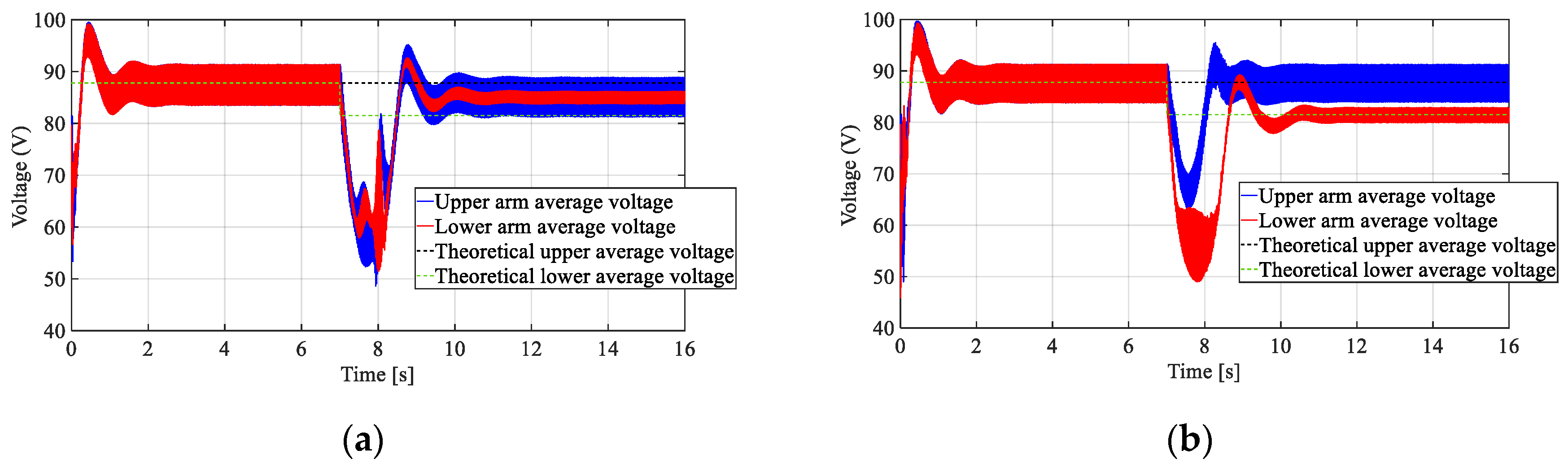
Looking at Figure 5, it is possible to recognize the different behaviors of the arm voltages for the two control strategies. In particular, in the time interval of 0–7 s, both of them practically give the same results in terms of both the powers and voltages of the PV modules. This is because the solar irradiation is the same for all the PV modules embedded in the arms. 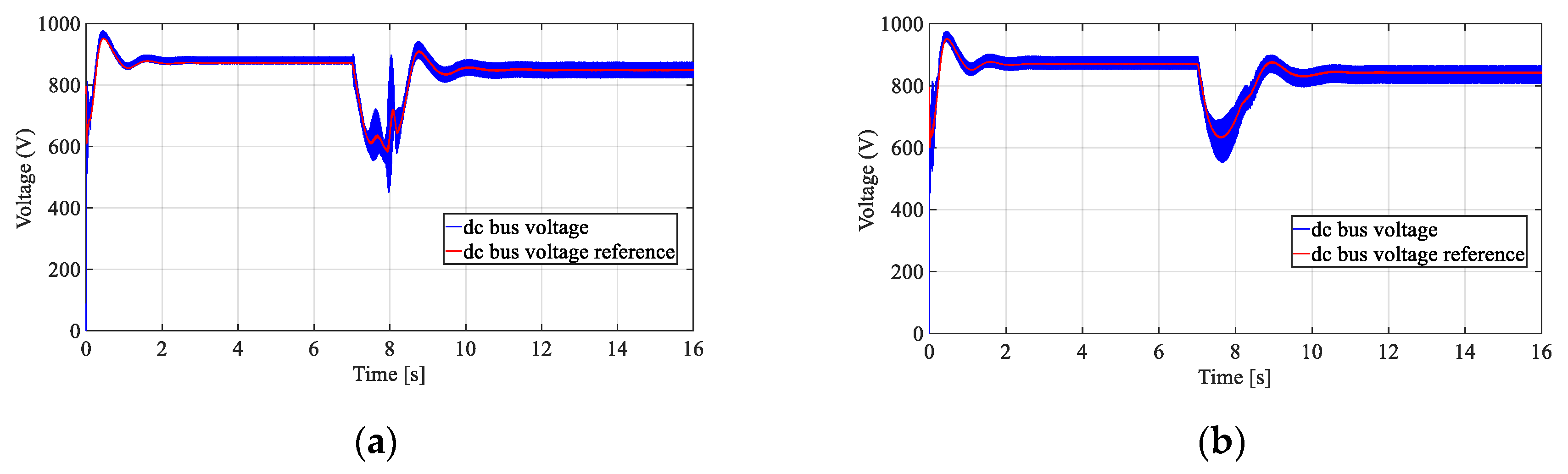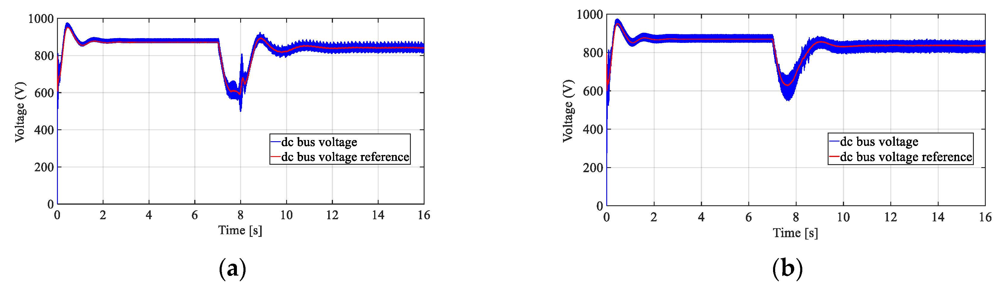On the other hand, in the time interval of 7–16 s, where the solar irradiation of all the PV modules of the lower arm falls to 300 W/m², the behaviors of the two controllers yield different results. In fact, the CMPPT controller forces the two arm voltages (upper and lower) to be equal because the difference between them is controlled to be zero. In the DMPPT controller, the arm voltages are instead free to follow their own theoretical voltages. In both cases, the dc bus voltage changes the steady state value based on the different irradiance conditions, as reported in Figure 6. 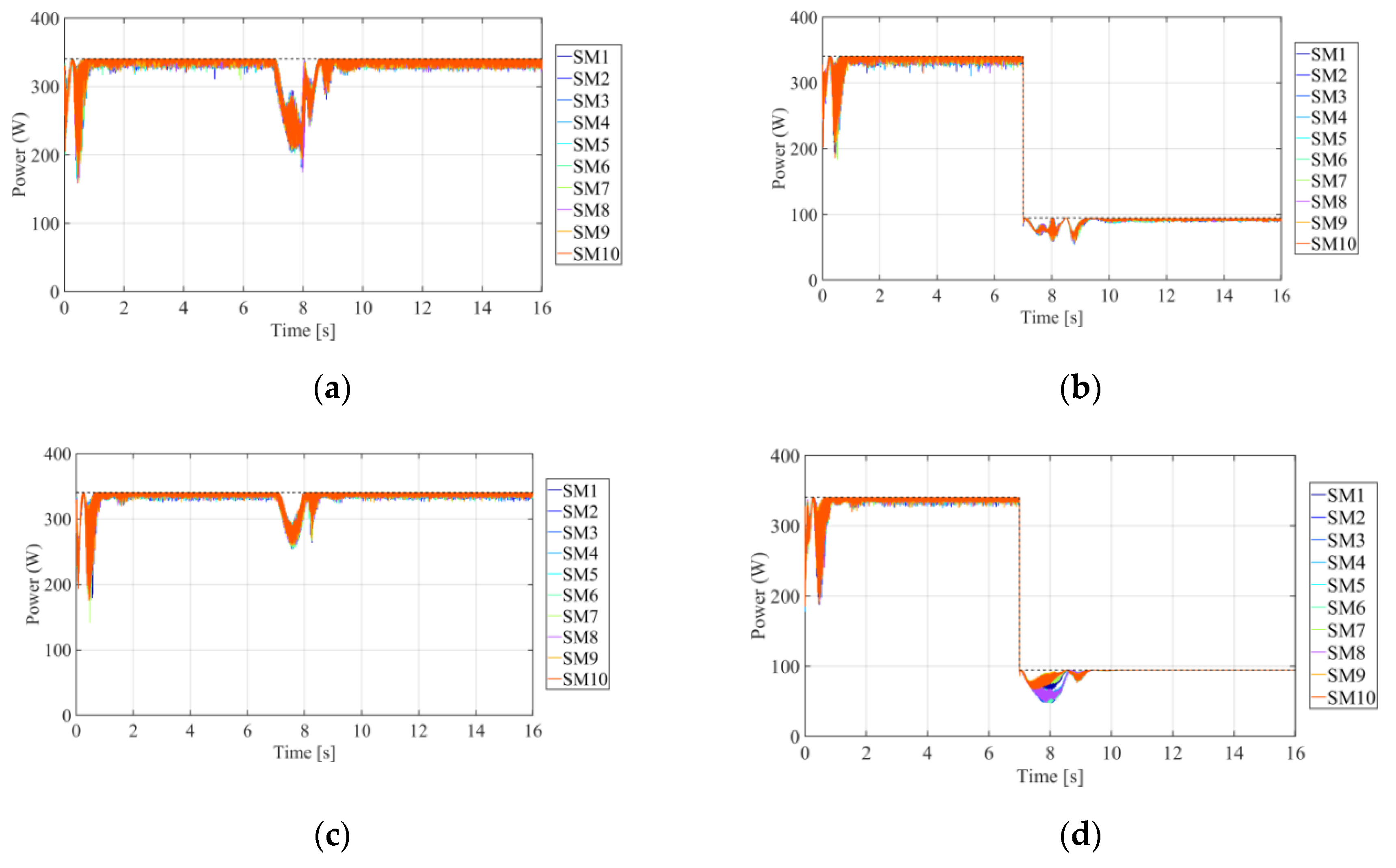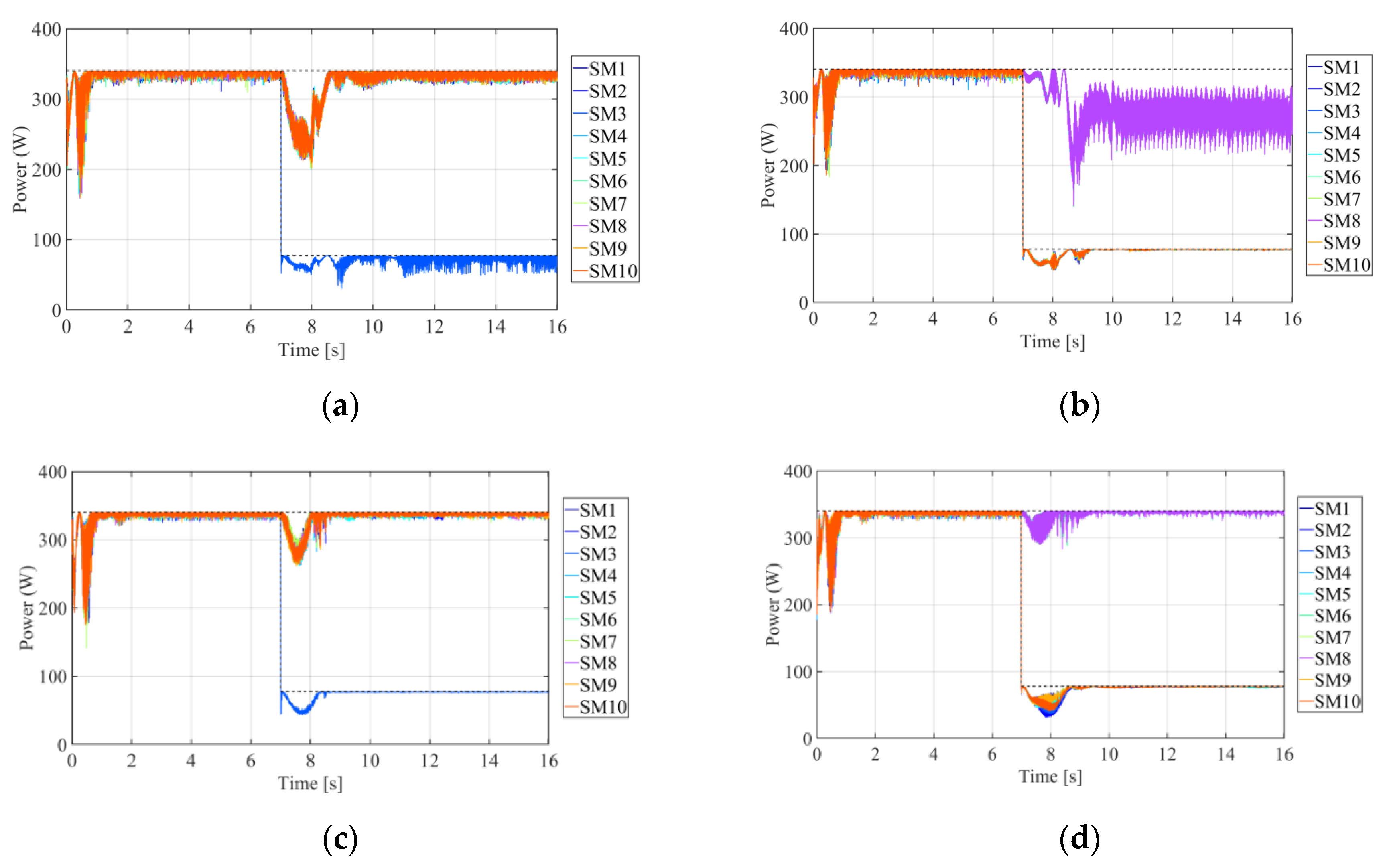Figure 7 shows the PV module powers for the two controllers compared with the maximum available powers (indicated as a black dashed line). The latter are related to the power that can be extracted from each PV module if they could work at their maximum power points. From this figure, we can note that the behaviors of the actual PV module powers in the time interval of 0–7 s are quite similar to each other. On the other hand, in the time interval of 7–16 s, where the power mismatch between the two arms appears, the DMPPT controller presents a better efficiency (calculated as the ratio between the sum of all the actual PV module powers and the sum of all the maximum available ones), because each arm can work at the proper theoretical average voltage.

5.2. Scenario 2. Different Partial Shading Conditions for One and between Arms

In this scenario, a partial shading condition between the two arms was analyzed. As in the previous scenario, in the time interval of 0–7 s, both arms were irradiated at the maximum value, i.e., 1000 W/m². Then, after 7 s, the solar irradiance was changed as reported in

Table 4. Scenario 2. Different partial shading conditions for both arms.

Submodule	Upper Arm		Lower Arm
	G(W/m2)
	t = 0–7 s	t = 7–16 s	t = 0–7 s	t = 7–16 s
SM1	1000	1000	1000	250
SM2	1000	1000	1000	250
SM3	1000	250	1000	250
SM4	1000	1000	1000	250
SM5	1000	1000	1000	250
SM6	1000	1000	1000	1000
SM7	1000	1000	1000	250
SM8	1000	1000	1000	1000
SM9	1000	1000	1000	250
SM10	1000	1000	1000	250

. The simulation results for the two control strategies are reported in Figure 8, Figure 9 and Figure 10.

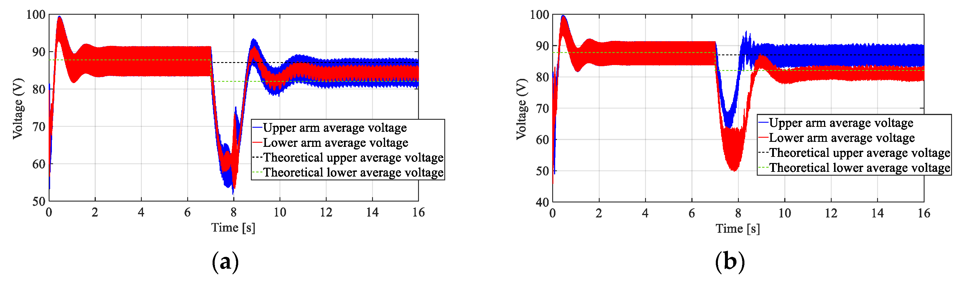
Looking at Figure 8, it is possible to recognize the different behaviors of the arm voltages for the two control strategies. In particular, in the time interval of 0–7 s, the controllers give practically the same results in terms of both the powers and voltages, as in the previous scenario. On the other hand, in the time interval of 7–16 s, the solar irradiation changes, causing a power imbalance between the two arms and in the arms themselves. Moreover, in this case, in the CMPPT controller, the two arm voltages are forced to be the same. In contrast, in the DMPPT controller, the arm voltages are free to follow their own theoretical voltages. As in the previous scenario, the dc bus voltage changes the steady state value based on the different irradiance conditions, as reported in Figure 9. 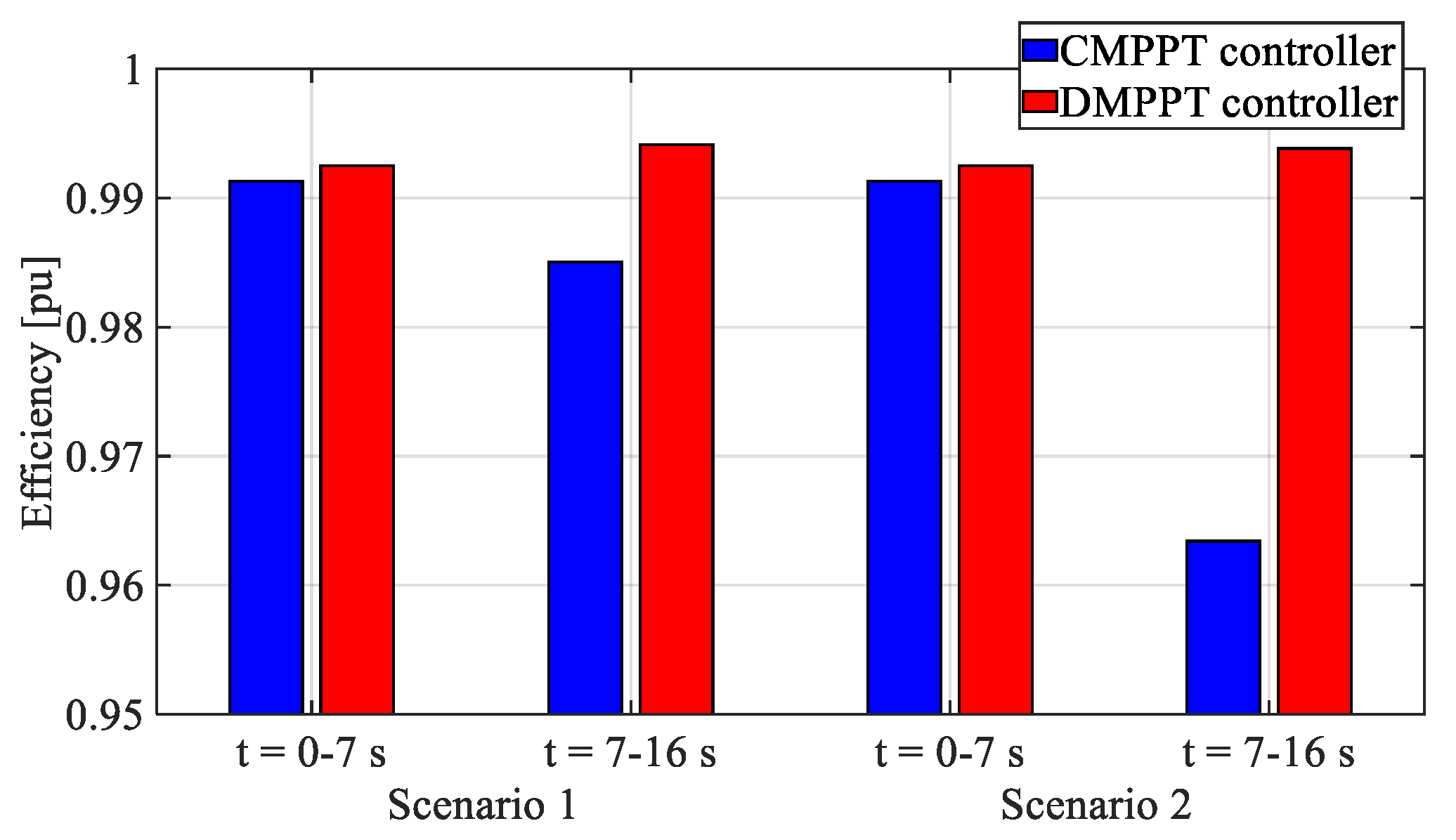Figure 10 shows the PV module powers for both controllers. From this figure, it is worth noting the robustness of the proposed DMPPT controller. Indeed, even under extreme unbalanced irradiance conditions, the DMPPT controller allows the entire system to work to the maximum power available. This is because each PV module can work at its own maximum power point voltage, which gives the maximum power. On the other hand, the CMPPT controller, as in scenario 1, forces the average arm voltages to be equal. At the same time, unlike scenario 1, where the inner solar irradiation for each arm is the same for all the PV modules, in this case, even the inner solar irradiance is different. Therefore, each PV module is influenced by the solar irradiances of the others. In this case, the CMPPT, making all the modules work at the same point, cannot ensure the full exploitation of the available power. This is clearly shown in Figure 11, where it is clear that there is a significant reduction in the MPPT efficiency for the CMPPT under unbalanced conditions. In contrast, the efficiency of the DMPPT is practically constant despite the unbalanced solar irradiation.

6. Conclusions

This study modeled a single-phase modular multilevel converter to integrate PV panels in the electrical grid. Moreover, a novel control strategy to obtain the maximum power available under any irradiance conditions was proposed. The proposed control strategy could decouple the control of the grid and circulating currents by changing the dc bus voltage based on the different irradiance conditions. In this way, each arm could work at its theoretical average voltage, allowing the system to show better performances. Moreover, the proposed submodule sorting algorithm compares each SM voltage of the MMC with its theoretical optimal one, which corresponds to the maximum power point voltage of the PV embedded module, allowing each PV module to work around its maximum power point. The validity of the proposed control strategy was demonstrated by comparing it with a conventional CMPPT controller. Different cases of solar irradiance, such as identical irradiance conditions for both arms, a partial shading condition for one arm, and different partial shading conditions for one and between the arms, were simulated. Under the same irradiance condition, both controllers achieve the same efficiency, but under unbalanced irradiance conditions, the DMPPT controller could produce higher output power close to the maximum available.