Drivers of CO₂-Emissions in Fossil Fuel Abundant Settings: (Pooled) Mean Group and Nonparametric Panel Analyses

1. Introduction

Oil-producing countries account for more than 30 percent of global greenhouse gas (GHG) emissions [1]. Countries such as Russia, Iran, Saudi Arabia, Mexico, and Indonesia belong to the top 20 countries with the largest aggregate carbon dioxide (CO₂) emissions worldwide [2]. With Saudi Arabia on the top, Russia, Iran, Mexico, Canada, and Brazil also belong to the list of the 20 countries with the largest per capita carbon emissions. The rest of the top carbon-emitting countries, both in cumulative and in per capita terms, are high income and high-middle income economies [3]. According to Herman Ott, climate scientist and lawyer at ClimateEarth, states abundant in fossil fuels have been systematically trying to block real action within the framework of the Kyoto Protocol and its successor, the Paris Agreement, by accusing the respective climate change action of heresy [4,5]. The potential losses due to the global energy transition due to the consequent reduction of the demand for oil and gas contribute to the obstruction of the deployment of carbon-saving technologies both within these countries and partly abroad over the investment activity of the sovereign wealth funds of the oil-rich countries.

The analysis of the intended nationally determined contributions (INDCs), i.e., the voluntary climate pledges of the oil-producing countries in the framework of the Paris Agreement, shows that oil producers differ in their mitigation strategies from the rest of the world. Their INDCs but also the work of the One Planet Sovereign Wealth Fund Working Group are mostly confined to the increase of renewables’ share in these countries’ energy mixes. By doing so, these countries first and foremost strive for the diversification of the national economies by producing photovoltaic systems and wind turbines. There are no noteworthy pledges of mitigation within the existing manufacturing or energy sectors over the carbon-saving innovations, reduction of the emissions by end consumers, or the carbon tax [1].

The literature on the drivers of environmental degradation in fossil-fuel producing and exporting countries is dominated by the parsimonious polynomial ‘black-box’ specifications that test the empirical validity of the environmental Kuznets curve conjecture. The ‘black box’ estimations with the average income as an omnibus variable enable only the assessment of the long-run income-environment relationship (IER). Such estimations allow no inference about the choice of concrete policies to mitigate environmental degradation. Besides, the use of the conventional panel regression techniques that ignore the time series traits of data, and the parametrization of economic specifications, i.e., pre-determinism, could lead to spurious estimators. To address these problems, this study employs the (pooled) mean group and nonparametric panel estimators.

Except Ike et al. [6], Esmaeli and Abdoullazadeh [7] and Sadik-Zada and Gatto [8], there is no study, which addresses the issue of GHGs in oil-producing countries. Nevertheless, all three surveys only assess the carbon footprint of the oil sector and the empirical validity of the environmental Kuznets curve (EKC) conjecture. Despite putting forward a sophisticated theoretical framework in Sadik-Zada and Gatto [8], their study enables only the compartmentalization of the GHG-footprint on the theoretical level and confines itself to the assessment of the bivariate IER.

In contrast, the paper at hand strives toward disentangling the sources of atmospheric pollution in the oil-abundant settings with a special focus on oil rent as a share of GDP and on sectoral structure, whereby the quantity of the carbon dioxide emissions serves as the proxy of the magnitude of atmospheric pollution. The findings of the study should contribute to the literature on global climate change mitigation. Choosing carbon dioxide as the dependent variable is in line with the notion of the global atmosphere as a sink for global GHGs [9]. Carbon dioxide is a long-lived climate pollutant and has been recognized in academia as the major driver of global climate change through its greenhouse effects. Sulfur oxides’ or oxides of nitrogen’s environmental repercussions are less severe in terms of global climate change. Methane, a short-lived climate pollutant, which also emanates inter alia from petroleum and especially combustion of the natural gas leads only to the temporary increase of the global temperatures [10,11].

This paper attempts to contribute to the literature on oil abundance and the environment in two ways. First, it represents a structuralist economic theory of natural resources-based development in terms of environmental degradation. The second contribution of this inquiry is empirical. This is the first study, which accounts for experimental evidence on the trade-off between multicollinearity and omitted variable bias. Therefore, it enables the identification of the major drivers of the carbon emissions in oil-producing economies and the reassessment of the EKC hypothesis in the respective context. The study makes use of the novel panel cointegration techniques, which account for the mixed-stationarity, panel heterogeneity, and endogeneity issues. Furthermore, to exclude the model misspecification problem, which is imminent in the parametric specifications, the study also employs novel nonparametric estimators, which are mostly in line with the panel cointegration estimators.

Turning the “black box” of the economy-environment relationship into a “white box” has practical repercussions for the policy formulation in the context of the national climate change mitigation policies in the fossil fuel reliant settings. The contemporary policymaking in the oil-rich settings lacks a reliable empirical basis for the scenario analysis of different environmental policy choices.

The remainder of the manuscript is organized as follows: The literature review in Section 2 analyzes the existing scholarship and puts forward the theoretical framework. Section 3 delves into methodological aspects of the inquiry, puts forward a multi-sector model of environmental degradation, and delineates the theoretical framework. Section 4 is dedicated to data issues. Section 5 presents the empirical estimation results. Section 6 elaborates on the implications of empirical findings and gives policy recommendations.

2. A Brief Literature Review

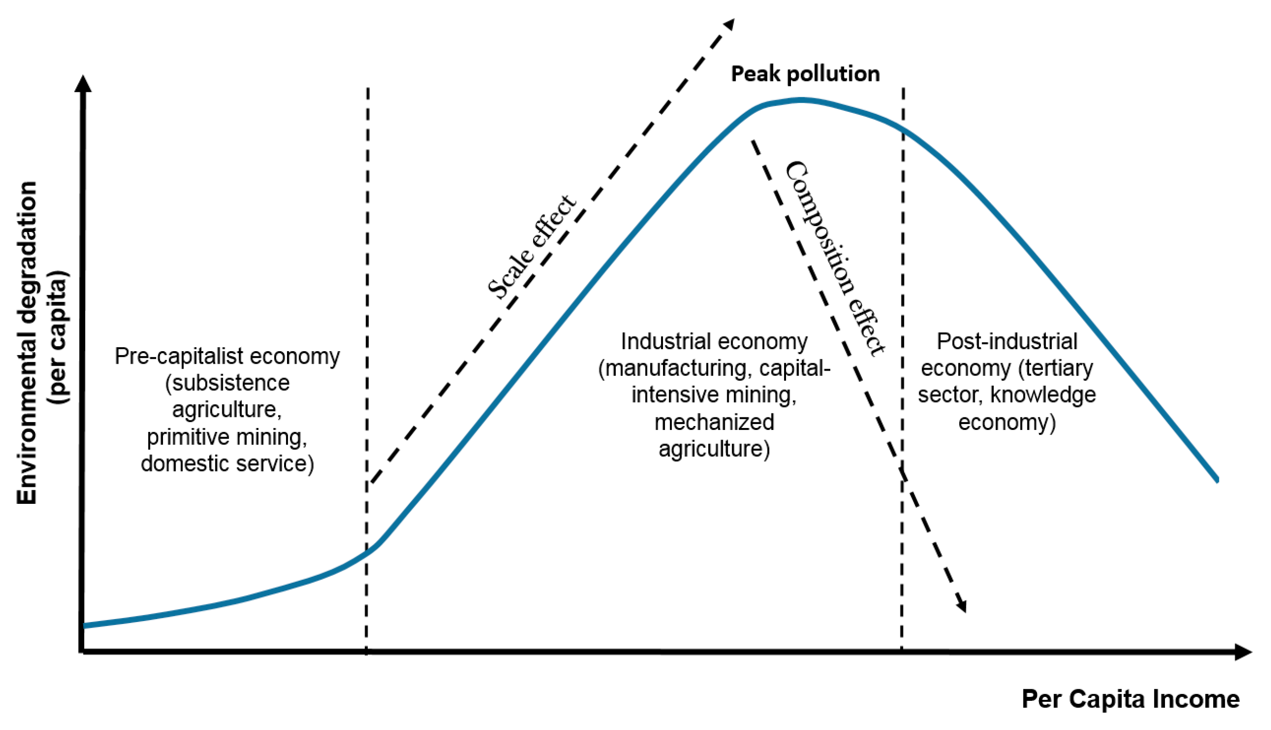
2.1. Income–Environment Relationship—The “Black Box”

The literature on the GHG-footprint of petroleum abundance is dominated by inquiries, which try to test the empirical validity of the inverted U-shaped income-environment relationship (IER), also referred to as the environmental Kuznets curve (EKC) conjecture, a paradigm that has been dominating the discussion on the economy–environment nexus for more than two decades. The EKC replaced the Impact-Population-Affluence-Technology (IPAT) equation in the mid of the 1990s, which presented a kind of neo-Malthusian view on environmental degradation.

The IPAT equation implies that the level or the magnitude of environmental degradation (I) can be explained by population growth (P); affluence (A), i.e., the level of income; and by the level of technological progress (T). All three drivers, population growth, the level of income, and technological progress, deemed to be contributors to the level of environmental degradation. For Ehrlich [12] in his bestseller The Population Bomb and Club of Rome’s Limits to Growth, technology has been considered as a factor with a negative or neutral impact on environmental amenities [13]. It seems that until 1973, the year of the first oil shock, the pollution-saving technological progress has not been considered at all in the realm of environmental economics and general technological progress had exclusively been taken as a pollution-augmenting phenomenon [9].

The pessimism of the Club of Rome has been first seriously contested by the Intensity of Use (IoU) hypothesis put forward by Malenbaum [14]. He detected an inverted U-shaped relationship between metal-intensity and average GDP. The arguments of the IoU hypothesis have been deeply rooted in the structural paradigm of economic development, whereby increasing material-intensity of the economy can be attributed to the level of economic development epitomized by the economic structure, i.e., sectoral composition of the economy [15,16,17,18,19]. In the early 1990s, the inverted U-shaped relationship was re-detected in the context of environmental degradation by Ehrlich and Holdren [20,21,22]. Panayotou [23] dubbed this empirical regularity the environmental Kuznets Curve (EKC) (Figure 1).

There are several common theoretical explanations for the existence of the inverted U-shaped IER. The first explanation is related to the changing structure of the economy [24]. In the process of transformation from being predominantly traditional to relying on industry and mechanized agriculture, environmental degradation in a country first increases [25,26] and later gradually falls during the displacement of carbon-intensive manufacturing by less carbon-intensive knowledge-based production [27]. Environmental upgrading, triggered by transformation of economic structure from mining and heavy industry toward the tertiary sector and knowledge economy development is known in the EKC-literature as the composition effect. Growing emissions at the early stages of economic development can be attributed to the development of mining and heavy industry. If the growing emissions are being induced by the growing level of per capita income then the increasing level of environmental pollution is the result of the so-called scale effect. According to the structuralist view of EKC-literature, at the early stages of economic development, the scale effect is the major driver of CO2 emissions as indicated by the upward sloping dashed arrow in Figure 1.

The second explanation, illustrated in Figure 1 by the downward sloping dashed arrow, claims that with an increasing standard of living people start to value environmental amenities more, which is expressed by an increased readiness to pay for a cleaner environment. In the mathematical models of resource use, this is usually reflected by increasing shadow prices of the stock of the natural environment [28]. This appreciation of the environment comes in its own in the settings with functioning democratic institutions and civil liberties [29].

The third explanation is tied to the investment in research and development (R&D), which takes place over-proportionately in high-income countries. The role of R&D investment as continuously fueling per capita income growth is the central aspect of models that have been embedded in the endogenous growth framework [30,31,32]. Rich nations afford more stringent environmental regulations and larger R&D investments in pollution-saving technologies, which induce more material- and energy-efficient economic growth [33].

The mentioned drivers of the inverted U-shaped IER are not mutually exclusive but rather complementary. In our opinion, the first-mentioned driver, the changing structure of the economy, triggered by the initial accumulation of capital and subsequent investment activities, is the primary cause of the inverted U-formed IUR. An increasing shadow price of the stock of the natural environment and an increasing leeway for R&D investments are repercussions of the industrialization-led increase of average income levels. Hence, in the following, we deem the changes in the valuation of environmental amenities and the introduction of carbon-saving technological progress as concomitants of economic modernization, which is epitomized in the changing sectoral composition of the respective economies [34].

2.2. Inside the “Black Box”

Sadik-Zada and Gatto [8] show that structural transformation could be gravely deformed by petroleum windfalls and could break the conventional pathways of decarbonization in the oil and gas exporting countries. The present study augments this theoretical framework by delving into the relationship between variations in the level of income and the tertiarization of the economy (Figure 2).

Fossil fuel combustion is responsible for about one-third of the anthropogenic CO₂ emissions ([35], p. 159). The petroleum value chain is the key driver of climate change [6,36]. The largest CO₂ emissions emanate from the oxidation of carbon, over fossil fuel combustion in power plants, oil refineries, and large industrial facilities. More than one-third of the GHGs in the oil-producing countries can be attributed to the petroleum value chains [37]. Nevertheless, these chains are not located exclusively in the oil-producing countries as all countries worldwide have their petroleum complexes. However, the two most energy- and carbon-intensive stages of the petroleum value chain, i.e., extraction and refinement stages, are mainly located within the oil-producing countries [38] where they contribute significantly to global GHG emissions (s. Figure 2, black arrows).

The petroleum value chain is certainly not the only source of the GHGs that is influenced by oil abundance. The influx of windfalls resulting from the exports of crude oil is another not less powerful channel, which is triggered by oil abundance. Such windfalls have strong fiscal linkage effects on the respective economies [39]. Especially since the inception of the boom phase of the latest commodity supercycle that started in the late 1990s, oil and gas revenues dominated the economies of the petroleum-exporting developing and transition countries. This dominance leads to grave consequences concerning the quality and dynamics of the structural change. The major implications of the resource curse (s. Figure 2, red arrows), the Dutch disease and the deterioration of the quality of political institutions, lead to the increasing costs, to the surge of the wage bill in the private sector, especially manufacturing [40,41]. As a result, internationally traded goods from manufacturing and agriculture lose their competitiveness on the international markets so that the local manufacturing and agriculture stagnates or even falls [42,43]. As mechanized agriculture and manufacturing are responsible for more than 30 percent of the emitted GHGs worldwide [44,45], the stagnation or contraction of these carbon-intensive sectors could lead even to a net decrease of GHGs [46,47].

Triggered by oil windfalls, the tertiary sector, and especially non-tradable services, are not exposed to this kind of competitive pressure and grow at a relatively high pace [48]. This contributes to the acceleration of the tertiarization, which is expressed in the growing share of the tertiary and stagnating share of the manufacturing sectors [40,41].

A further consequence of fossil fuel abundance is related to the social transfers and subsidization of cheap oil and fossil-fueled power for intermediary inputs and end consumption. The Fossil Fuel Subsidies Database of the International Energy Agency (IEA) shows that oil-exporting developing countries’ fossil fuel subsidies in per capita terms are a tenfold of that of oil-importing developing countries [49]. With the level of subsidies of 1308 USD per capita, Kuwait has the greatest fossil-fuels subsidies worldwide, Iran, with 1038 USD per capita comes second, and Saudi Arabia comes third with a per capita subsidy of 838 USD. In essence, this kind of subsidization is tantamount to a negative carbon tax. This indicates that oil-rich countries do not follow just lax environmental regulations, but, in contrast to oil importers, even subsidize atmospheric pollution [48]. This kind of policy supports energy-intensity and the surge of fossil-fuel combustion-based power and heat generation and fuels GHG emissions (s. Figure 2). The world electricity production during the last five years has largely been driven by oil-producing countries, which generated electricity mostly in oil-fueled power plants, as reported by Enerdata [50].

The above-presented review reveals that there are several channels, through which oil abundance shapes global atmospheric pollution, which emanates from oil-rich countries. These include the petroleum value chain’s direct emission effects, the oil-growth nexus, and especially Dutch disease, the massive subsidization of fossil-fueled thermal power and heat generation, and the pre-mature de-industrialization theses [51,52]. Figure 2 combines these different perspectives and outlines the conceptual framework of our analysis, which we will use in the following sections to answer the following questions:

Q 1:

Does the inverted U-shaped IER hold in the case of the oil-producing countries?

Q 2:

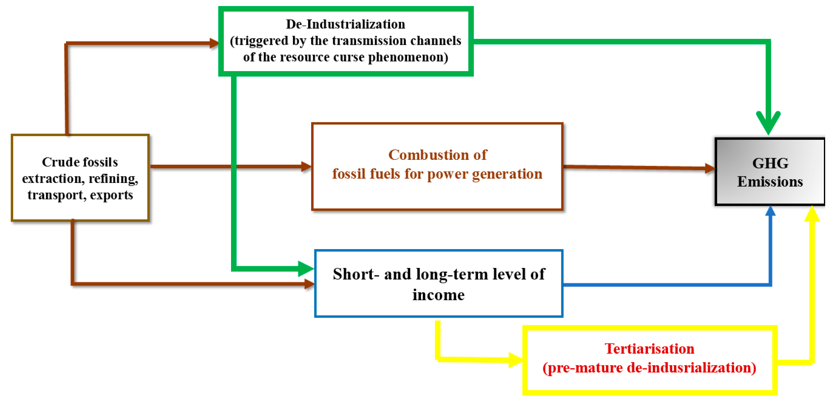
What is the net carbon-footprint of fossil-fuel abundance on the level of carbon dioxide emissions?

Q 3:

What are the essential drivers of carbon dioxide emissions in oil-producing countries?

Given the significance of oil-producing countries’ role in global atmospheric pollution and the complexity of the oil sector-GHG nexus, addressing the above-listed questions means dealing with a topic of considerable relevance for global debates on the mitigating climate change. Answering these questions requires the identification of the net and disentangled GHG-footprint of oil abundance, which by far from trivial and necessitates a sophisticated empirical approach. The next subsection is dedicated to these issues.

3. Methodology

In this subsection, first, we briefly discuss the collinearity and confounding variables that emanate from the proposed conceptual framework in the light of the latest experimental findings in this regard. In Section 3.2, we present the polynomial regression estimation procedure and related problems. Section 3.3 illustrates a nonparametric panel regression approach.

3.1. Multicollinearity and Confounding Variable Issues in Ecological Analyses

In contrast to ‘black-box’-dominated studies to test the validity of the EKC hypothesis, applied ecological research usually employs multiple regression approaches [53,54]. The central problem of multiple ecological regressions is that ecological response variables depend on explanatory variables that are often multicollinear, i.e., correlated with each other.

This study is confronted with both multicollinearity and confounding variable problems. As shown in Figure 2, de-industrialization, the level of per-capita income and tertiarization are interrelated. This is an indication of the existence of multicollinearity at the theoretical level. The variation inflation factor (VIF) for the set of variables, which is predicated on the theoretical framework indicates a VIF of 3.66 (s. Appendix A.1). The correlation matrix of coefficients of the xtpmg model, which will be employed in the following subsection, gives fairly light indications for the existence of multicollinearity (s. Appendix A.2).

Crude oil production in Figure 2 affects GHGs (dependent variable) both directly over the oil value chain and indirectly over other dependent variables. Hence, there exists a confounding variable problem too. Also, it can be assumed, that especially in the case of the less developed countries, the oil sector emanates strong production and fiscal linkage effects that dominate the whole economy. This is the essential determinant of all the processes in the respective economies. Literature shows that this assumption holds for most oil-dependent developing and transition economies.

Literature associates multicollinearity with a higher coefficient of determination; low t-values of the variables; statistical insignificance of relevant variables; an incorrect sign of the coefficients; and substantial volatility in parameter estimates [55,56,57]. VIF is the ratio of variance with many independent variables by the variance of the regression with just one variable. A VIF of n implies that the variance of i-th coefficient is n times greater than in the case with no multicollinearity [58].

In Greene [56], Wooldridge [59], Rogerson [60] and Menard [61], and Petraitis et al. [62], VIFs of over 20, over 10, over 5, and 2, respectively, have been indicated as the thresholds for strong multicollinearity. All these thresholds, however, are arbitrary without any theory behind them. Hence, there is no generally accepted threshold of VIF in the literature [63].

To account for multicollinearity, the researchers often exclude the variables inducing interdependence of the predictors and leave only essential independent explanatory variables [54,64,65]. In contrast to applied ecological surveys, economics, and business administration studies, elimination of the variables with large partial correlations with other variables is the most proliferated methodology in reducing collinearity [64,65,66].

This procedure reduces multicollinearity but at the same time contributes to the omitted variable bias and thus, can cause a substantial reduction of the explanatory power of econometric analyses [53,67]. Furthermore, the elimination of one or more predictors alters the theoretical foundations of econometric specifications [68].

Lindner et al. [67] and Wooldridge [59], nevertheless, contest the critical stance towards multicollinearity and discourage applied researchers from eliminating interdependent predictors from econometric specifications. According to Allison [69] and Lindner at al. [67], the omission could lead to even more detrimental consequences in terms of the efficiency of the estimations than collinearity itself. In their simulation studies, collinearity of the variables led to the inflation of standard errors and at the same time contributed to the efficiency of the estimators, if the variables were relevant. Graham [54] shows that, especially in ecological forecasting, whereby the target is the prediction of the dependent variable, the correlation between the variables on the right-hand side of the estimation equation does not diminish the predictive capability of the model.

Gordon [70] proposed a more elegant solution of collinearity by combining two or more highly correlated variables as one variable. This is a kind of composite index building strategy, which also corresponds with a myriad of methodological problems related to the unified scaling of the variables [71].

Furthermore, there is also another issue, namely, the confounding variable problem, if there exists a variable that influences both dependent and independent variables. Ignoring such a variable could lead to over- or underestimation of the strength of the independent variables and/or a change of the sign of an effect [59].

Another econometric issue, which is more important for the forecasting of the IER has been indicated in Bertinelli and Strobl [72] and later in Azomahou et al. [73]. The studies indicate that despite some important merits, confinement of the specifications to just one independent variable, per capita income, alters the speed of convergence, i.e., the adjustment term.

The paper at hand makes the first step toward breaking the dominance of the bivariate black-box approach and employs both bi- and multivariate regressions to analyze the forces that drive carbon emissions in the oil-producing countries.

3.2. Parametric Specification

Our empirical strategy for the assessment of Q1 and Q3 is in line with Calvancanti et al. [60] and is based on the following model specification:

$$\begin{array}{ll}\ln C{O}_{PC}{}_{it}=& a_j+{\beta }_1\text{ln}{(PCI)}_{it}+{\beta }_2{{\ln }_{}}_{}{\left(PCI\right)}_{it}^2\\ & \hspace{1em}\hspace{1em}+{\beta }_{3}Power from Fossil{s}_{it}+{\beta }_{4}Teriarizatio{n}_{it}\\ & \hspace{1em}\hspace{1em}+{\beta }_{5}Manufacturin{g}_{it}+{\beta }_6{\left(Oil Rent\right)}_{it}+{\beta }_7{\left(Oil Rent\right)}_{it}^2+u_{it}\end{array}$$

(1)

where $a_j$ denotes country-specific fixed effects iable, $PC{I}_{it}$ is the indicator for per capita income, $PC{I}_{jt}^2$ is the second control variable, which indicates the squared value of per capita GDP, Power from Fossils is the share of fossil-based electricity in total electricity production, Tertiarization is the share of services sector value added in GDP, Manufacturing is the absolute value of the manufacturing value-added, $Oil Rent$ is the share of oil rent in GDP and ${\left(Oil Rent\right)}^2$ is oil rent’s squared value for countries $i=\overline{1,J}$ and time periods $t=\overline{1,T}$, and $u_{it}$ is the error term.

For the assessment of Q2, the net carbon footprint of oil, the study employs the ‘black box’ approach. The corresponding econometric specification reads as follows:

$$\ln C{O}_{PC}{}_{it}=a_i+{\beta }_1\ln \_Oi{l}_{it}+u_{it}$$

(2)

The advantage of the parsimoniousness of the model is that the broad number of country-specific time-irreversible factors are captured by the country-specific deterministic factor, $a_i$. The same holds for $u_{ij}$ concerning the unobserved common factors [60].

3.3. Pooled Mean Group Estimators and Dynamic Fixed Effects

The central advantage of the pooled mean group (PMG) approach panel cointegration approach is that the PMG estimators, in contrast to the conventional fixed and random effect panel estimators, account for the time series characteristics of the panel data sets. The unique methodology proposed in Pesaran et al. [74] accounts for panel heterogeneity, endogeneity of variables and allows mixed-stationary, i.e., the mixture of the I(0) and I(1) processes in the same estimation equation. In addition, the underlying autoregressive distributive lag model (ARDL) allows for disentangling the short- and long-term effects, differences in error variances, and the intercepts [75]. The further advantage of the PMG procedure over other panel estimation methodologies is its robustness to the outliers and lag orders. The PMG estimator also accounts for the heterogeneity in the short-run responsiveness, error variances, and the intercepts in the panel datasets [76]. This is the reason for the increasing popularity of the PMG-estimators for the assessment of the IER since the mid-2000s [77,78,79].

Until now, the issue of environmental pollution in petroleum-producing countries has not been addressed within the PMG framework. PMG assumes a heterogeneous short-term and homogenous long-term response, i.e., cointegrating vector, across the panel. A similar estimator, the mean group (MG) approach, assumes that both short- and long-term responses across the panel are heterogeneous and calculates country-specific short- and long-term coefficients. We decide to use a PMG estimator based on the Hausman test statistics. The study employs dynamic fixed effects (DFE) in cases, whereby due to computational reasons the employment of (P)MG fails. Like PMG, DFE also restricts the cointegrating vector to be equal across countries. In addition, DFE restricts the speed of adjustment term and short-run coefficients to be identical for all panels [80].

3.4. Nonparametric Fixed Effect Panel Analysis

The use of parametric regression models is justified, if the function that describes the relationship between dependent and independent variables is known. It is well established that parametric regression models may cause model misspecification [81]. Bradley and Srivastava [82], and Brauner and Shacham [83], show, nevertheless, that collinearity among the independent variables in the polynomial regression models may substantially confine the predictive capabilities of these models by yielding inconsistent estimators [84,85]. Furthermore, parametric analyses, especially in the context of climate change research, reveal that these models often do not approximate the relationship between the variables [86]. Hence, in the framework of our analyses, nonparametric trending models, which enable the data to “speak for themselves” are superior to parametric linear and polynomial models [87,88]. Despite its proliferation for the analysis of the cross-sectional and time series analysis, nonparametric and semi-parametric data analysis for panel data came to their own only after publication of Li et al. [84]. The paper at hand employs the nonparametric time-varying coefficient panel data model with fixed effects suggested there.

To obtain the nonparametric time-varying coefficients based on the panel data analysis with fixed effects we utilized the Stata module xtnptimevar. These estimators assess the effects of the independent variables on the dependent variables in a nonlinear fashion in the context of the panel data without imposing a specific functional form. In other words, they want the data to reveal the functional form by letting the data speak for itself. The command xtnptimevar exactly does that. It offers two estimators: the local linear dummy variable estimator (the default) and the averaged local linear estimator. Both of these techniques allow for estimating coefficients that vary over time for panel data models [89].

The nonparametric trending time-varying coefficient panel data model has the following form

$$Y_{it}=f\left(t\right)+X_{it}^T{\beta }_t+{\alpha }_i+u_{it}$$

(3)

where $f\left(t\right)$ are unknown functions. In the case of this inquiry, $f\left(t\right)$ are unknown country-specific trend functions; ${\beta }_t={\left({\beta }_{t,1}, \dots , {\beta }_{t,k}\right)}^T$ is an unknown vector of time-varying coefficients; $a_i$ represents unknown individual effects; and $u_i$ is stationary for each $i$; $T$ is the time series length and $N$ is the cross-section size. The proposed model is a fixed-effects model if ${\alpha }_i$ is allowed to be correlated with $\left\{X_{it}\right\}$ with a non-specified correlation structure [88,89]. Furthermore, for the sake of identification, it is assumed that ${\displaystyle \sum }_{i=1}^N{a}_i=0$ and that the time variable T is scaled by T, such that $f\left(t\right)=f\left({\tau }_t\right)$ and ${\beta }_t=\beta \left({\tau }_t\right)$, whereby ${\tau }_t=t/T\in \left[0,1\right]$ [87].

Following Su and Ullah [83] and Sun et al. [84] and based on comparisons between the averaged local linear estimates (ALLE) and local linear dummy variable estimates (LLDVE), Li et al. [90] proposed the LLDVE as a superior procedure in terms of the rate of convergence for the coefficient function. Both ALLE and LLDVE remove fixed effects by deducing a smoothed version of the cross-time average from each panel [90]. LLDVE is based on the following three assumptions. These are:

(1) $X_{it}$ and ${\alpha }_i$ can be correlated; (2) $u_{it}$ may be cross-sectionally dependent for each $i$ and independent of $X_{it}$; and (3) $u_{it}$ is in line with certain martingale difference conditions concerning time [85]. The bandwidth selection and bootstrapping of the confidence intervals is efficiently exhibited for an analogous survey in Silvapulle et al. [91].

The nonparametric estimations presented in this subsection complement the PMG, MG and DFE estimations by analyzing the aspect that cannot be analyzed in the framework of the parametric research, i.e., the time-varying impact of variations in income, oil-dependence, power and heat generation, and of tertiarization on the carbon footprint.

4. Data

The data structure is a balanced panel of 37 oil-producing and exporting countries in the time interval spanning between 1989 and 2019. The list of countries is provided in Appendix A.3. All the variables except for the Political Rights Index (PRI) and Civil Liberties Index (CLI) have been provided by the World Bank, World Development Indicators. PRI and CLI data have been prepared by the Freedom House. The employed data series and their transformations have been outlined in the following

Table 1. Description of data.

Variable	Description/Transformation	Source
LN_CO2_PC	Per capita carbon dioxide emissions. Carbon dioxide emissions are those stemming from the burning of fossil fuels and the manufacture of cement. They include carbon dioxide produced during consumption of solid, liquid, and gas fuels and gas flaring.	World Development Indicators 2020
LN_PCI	Natural logarithm of GDP per capita. GDP per capita is gross domestic product divided by midyear population. GDP is the sum of gross value added by all resident producers in the economy plus any product taxes and minus any subsidies not included in the value of the products. It is calculated without making deductions for depreciation of fabricated assets or depletion and degradation of natural resources. Data are in constant 2010 U.S. dollars.	World Development Indicators 2020
LN_PCI2	Natural logarithm of the squared value of per capita GDP.	World Development Indicators 2019
LN_Oil_Sh	Share of oil rents in total GDP. Oil rents are the difference between the value of crude oil production at world prices and total costs of production.	World Development Indicators 2019
LN_MVA	Natural logarithm of the Manufacturing Value Added. Manufacturing refers to industries belonging to ISIC divisions 15–37. Value added is the net output of a sector after adding up all outputs and subtracting intermediate inputs.	World Development Indicators 2020.
Ln_Tertiarization	Natural logarithm of the share of services as a share of GDP. Services correspond to ISIC divisions 50–99 and they include value added in wholesale and retail trade (including hotels and restaurants), transport, and government, financial, professional, and personal services such as education, health care, and real estate services.	World Development Indicators 2020.
LN_POWER_FOSSILS	Natural logarithm of the share of electricity production from fossil fuels in total electricity production. Sources of electricity refer to the inputs used to generate electricity. Oil refers to crude oil and petroleum products. Gas refers to natural gas but excludes natural gas liquids. Coal refers to all coal and brown coal, both primary (including hard coal and lignite-brown coal) and derived fuels (including patent fuel, coke oven coke, gas coke, coke oven gas, and blast furnace gas). Peat is also included in this category.	World Development Indicators 2020.
Political Rights Index	The Political Rights index measures the degree of freedom in the electoral process, political pluralism and participation, and functioning of government. Numerically, Freedom House rates political rights on a scale of 1 to 7, with 1 representing the most free and 7 representing the least free.	The Freedom House 2020.
Civil Liberties Index	The Civil Liberties Index is a composite index that measures the degree of civil liberties. Numerically, Freedom House rates civil liberties on a scale of 1 to 7, with 1 representing the most free and 7 representing the least free.	The Freedom House 2020.

.

The study makes use of the elaborations in Törnqvist et al. [92] and the findings in the follow-up inquiry in Gerdes [93], which show that in the context of the panel regression analysis, working with the logarithmic share variables yields more efficient estimation results, rather than actual shares when estimating fixed-effects models. Gerdes [93] shows that the linear estimator inversely weights variations in shares by its denominator.

In the face of the asymmetry of the linear estimator, the implicit weighting of the share variables paves the way for the spurious correlation between the share and the dependent variable and systematic measurement errors [93,94,95]. Hence, to avoid spurious results caused by the combination of shares and fixed effects, the study employs logs of the shares of oil rents, tertiary sector, and fossil fuels as independent variables [96].

Furthermore, because the shares of the manufacturing and tertiary sectors’ shares in total GDP are complements, to avoid collinearity the study employs the log-share of the tertiary sector in GDP and the natural logarithm of the absolute value-added of the manufacturing sector as dependent variables.

5. Estimation Results

5.1. Parametric PMG Regressions

In this subsection, the study presents the MG, PMG, and the DFE estimators. Before employing these panel cointegration estimators, the study tested the time series for the existence of the unit-roots and cross-sectional dependence. The Fisher-type panel unit root tests with zero and one lag indicate that the series are I(0) and I(1) processes. None of the series is integrated of order two, i.e., I(2) processes. The unit root test statistics are reported in the Supplementary Materials. This allows for the application of the mentioned estimators. Pesaran test for weak cross-sectional dependence [97] indicates that in the case of all econometric models, the null of “errors are weakly cross-sectional dependent” is rejected at the one percent level, The test statistics are reported

Table 2. Panel Cointegration Estimators, 1989–2019.

DEPENDENT VAR: CO2EMISSIONS PER CAPITA	Model 1 (PMG)		Model 2 (PMG)		Model 3 (MG)		Model 4 (PMG)		Model 5 (DFE)		Model 6 (DFE)		Model 7 (DFE)
VARIABLES	Long-Term	Short-Term	Long-Term	Short-Term	Long-Term	Short-Term	Long-Term	Short-Term	Long-Term	Short-Term	Long-Term	Short-Term	Short-Term	Long-Term
Adjustment Term (ec)		−0.252 ***		−0.271 ***		−0.671 ***		−0.316 ***		−0.305 ***		−0.393 ***	-0.352 ***
		(0.0395)		(0.0402)		(0.0678)		(0.0572)		(0.0258)		(0.0327)	(0.0331)
D.lnOil_Sh		0.0283		0.0144		−0.0146		0.0270		0.003		−0.00379		−0.014
		(0.0273)		(0.0193)		(0.0289)		(0.0197)		(0.0132)		(0.0153)		(0.0146)
lnOil_Sh	0.126 ***		0.0634 ***		0.108 **		0.0287 ***		0.0633 **		0.0537 **		0.102 ***
	(0.0164)		(0.0184)		(0.0523)		(0.00995)		(0.0277)		(0.0233)		(0.023)
L2.lnOil2			0.0437 ***		0.00843
			(0.00901)		(0.0240)
L2D.lnOil2				−0.0180 **		−0.0115
				(0.00820)		(0.00890)
ln_PCI					0.666 **		0.567 ***							0.274 ***
					(0.266)		(0.0252)							(0.095)
D.ln_PCI						0.340 *		0.447 **					0.248 *
						(0.182)		(0.212)					(0.1430)
ln_Power_fossils							0.265 ***		0.090 *		0.0692 *			0.028
							(0.0450)		(0.0498)		(0.0408)			(0.0401)
D.ln_Power_fossils								−19.46		0.042 *		0.0355	0.051 ***
								(18.85)		(0.0221)		(0.0230)	(0.204)
ln_Tertiary									0.312 ***		0.125 *			−0.003
									(0.0567)		(0.074)			(0.004)
D.ln_Tertiary										0.193 *		0.357 ***	0.001
										(0.1935)		(0.1479)	(0.0019)
lnMVA											0.299 ***			2.47 × 10−12 *
											(0.0849)			(1.49 × 10−12)
D.lnMVA												−0.0466	1.28 × 10−12
												(0.0863)	(1.36 × 10−12)
Political Rights Index														−0.065 *** (0.0217)
D. Political Rights Index													0.016 (0.117)
Constant	0.191 **		0.178 **		−3.941 **		−1.665 ***		−2.199 ***		−3.844 ***			0.588 ***
	(0.0965)		(0.0899)		(1.611)		(0.310)		(0.4719)		(0.663)			(0.3149)
Observations	812		745		729		702			-	-		-
Hausman ${\chi }^2\left[p>{\chi }^2\right]$	H0: PMG/H1: DFE		H0: PMG/H1: DFE		H0: PMG/H1: MG		H0: PMG/H1: MG		H0: MG/H1: DFE		-		-
	0.26		0.10		1.67		0.13		0.00
	$\left[0.6124\right]$		$\left[0.9497\right]$		$\left[0.6435\right]$		$\left[0.9878\right]$		$\left[1.000\right]$
Pesaran CD test statistics	46.7		39.3		58.1		51.7		57.9		44.1		38.08

Notes: (P)MG stands for (Pooled) Mean Group estimates and DFE denote Dynamic Fixed Effects. Standard errors are given in parentheses. CD stands for Pesaran’s Cross-sectional Dependence test proposed in Pesaran (2004). Standard errors in parentheses. *** p < 0.01, ** p < 0.05, * p < 0.1

. Hence, it is not required to employ Common Correlated Effects versions of MG, PMG, and DFE estimators [98].

Furthermore, for the test of the structural breaks the study employed the Clemente–Montañes–Reyes double additive outlier unit root tests structural break tests for each of the 37 countries. The test statistics are available as Supplementary Materials. We find that for most of the countries, 1994 and 2006 were the years of the structural change concerning carbon dioxide emissions. Because of the strong indications of the structural breaks, the study employed the Westerlund panel cointegration tests, which is compatible with structural breaks. The Westerund test indicates that all the variables are cointegrated. This non-compulsory test shows additionally that the series are cointegrated. The (P)MG and DFE estimators also confirm the validity of cointegration between the variables. All the adjustment terms are statistically significant and negative. The inclusion of the additional independent variables in the estimations in the PMG estimations leads to the slight increase of the adjustment speed from −0.252 to −0.316. The MG estimator, the third model in Table 2, with −0.671, is much greater than that of the other models. This is nevertheless, typical, that the adjustment parameter of the MG models is higher than that of PMG.

Both the parsimonious PMG-Model 1 and multiple regression models, PMG-Model 2, MG-Model 3, PMG-Model 4, DFE-Models 5 and 6 indicate that a greater share of oil rents in GDP in the long-run corresponds with more carbon emissions. One percent increase of the share of oil rents as a share of GDP leads to a 0.0287–0.126 percent increase of the per capita ${\mathrm{CO}}_2$ emissions. The estimations find no statistically significant short-term impact of the varying share of oil rents in GDP on emissions. PMG-Model 3 indicates that the squared value of oil rents as a share of GDP has no statistically significant impact on the level of per capita carbon dioxide emissions. The statistical significance in the PMG-Model 2 vanishes after controlling for per capita income (PCI) in the MG-Model 3. MG-Model 3 and PMG-Model 4 indicate that the average income has a statistically significant positive short- and long-term effect on per capita ${\mathrm{CO}}_2$ emissions. One percent increase of PCI leads in the long-run to 0.567–0.666 percent increase of average ${\mathrm{CO}}_2$ emissions. In the short run, one percent increase of average income leads to 0.340–0.447 percent increase of per capita ${\mathrm{CO}}_2$ emissions. DFE-Models 5 and 6 indicate that tertiarization also has a statistically significant positive short- and long-term impact on carbon emissions: one percent increase of tertiary sector as a share of GDP leads in the long-run to 0.125–0.312 percent and in the short-run to 0.193-0.357 percent increase of the per capita ${\mathrm{CO}}_2$ emissions. The tertiary sector, nevertheless, does not have a statistically significant impact on the level of per capita ${\mathrm{CO}}_2$ emissions. Manufacturing sector output has a statistically significant long-term effect on per capita ${\mathrm{CO}}_2$ emissions: a one percent increase of manufacturing value-added leads to a 0.299 percent increase of per capita ${\mathrm{CO}}_2$ emissions. The parsimonious PMG estimations with the squared value of average income do not validate an inverted U-shaped income-emissions relationship (see Appendix A.4). One percent increase of average income leads to 0.872 percent increase in the per capita ${\mathrm{CO}}_2$ emissions. Hence, both multivariate and parsimonious approaches, indicate a strong validation for the monotonically increasing income-emissions relationship. The EKC conjecture has been convincingly rejected.

In DFE-Model 7 the study controls for the role of political freedoms by adding Political Rights Index of The Freedom House. This is in line with the findings in Panayotou [99], Bhattarai and Hammig [100] and Dutt [101]. The model shows that increasing level of political freedoms corresponds with decreasing per capita carbon dioxide emissions. If index increases by one unit then we would expect the per capita CO₂ emissions to decrease by 6.5 percent. This implies that societies with a greater magnitude of political freedom (less index value) correspond with more, and countries with less political freedoms correspond with fewer emissions. Testing the effect of civil liberties by using the Civil Liberties Index of The Freedom House yields analogous results. The results with both Political Rights Index and Civil Liberties Index exhibit both concerning the coefficient significance and sign-stability robust (Estimation with Civil Liberties Index as independent variable are reported in the Supplementary Materials). These results are not in line with the state of the art, which indicates a positive relationship between better institutions and environmental upgrading. The literature on the positive nexus between institutional quality and environmental upgrading is mostly confined to OECD countries [9]. All the countries, with the only exception of Norway, belong to the group of the developing and transition economies. This could be the reason, why in the context of the oil-rich developing countries a greater level of democracy does not translate to greater environmental protection. On the contrary, countries with less democratic freedoms in tendency have less per capita emissions. Autocracies in the MENA region, Sub-Saharan Africa, and Central Asia are favorable toward environmental protection and implement large-scaled environmental upgrading projects in collaboration with the UN-institutions that contribute substantially to the positive image of ruling state elites. Independent of the motives of the ruling elites in the oil-exporting countries, both national and multilateral development agencies should make use of the respective governments’ positive stance towards environmental protection and enhance new joint projects and the projects within commitments related to Paris Agreement.

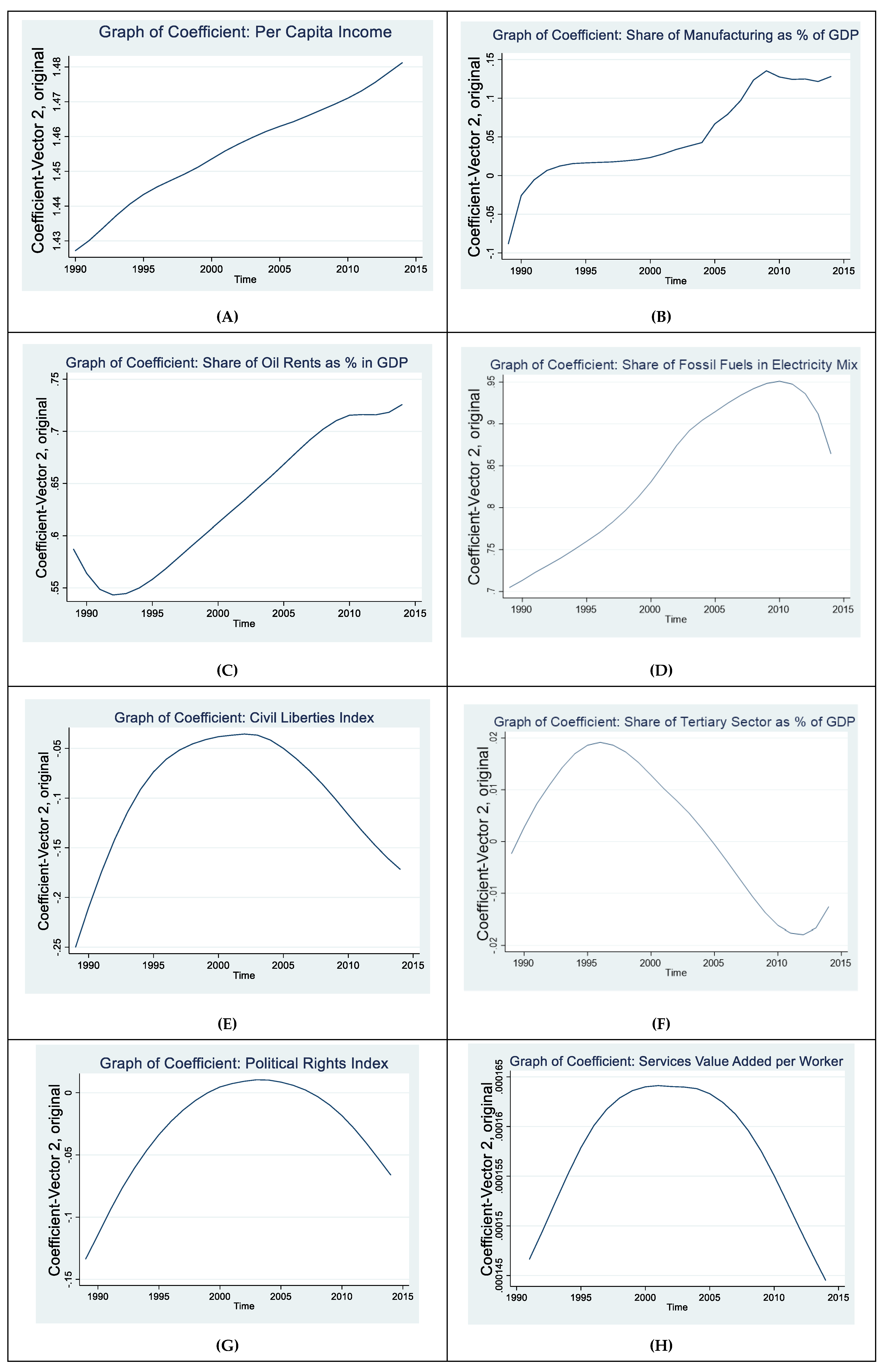
5.2. Nonparametric Analysis

As already mentioned, the nonparametric time-varying coefficients panel data analysis with fixed effects does not impose a priori a specific functional form for the relationship between the variables of interest. Furthermore, nonparametric estimators assess the changing responsiveness of the dependent variable (here in all the estimations the natural logarithm of the per capita carbon dioxide emissions) to the marginal changes of the independent variables [102]. Assessment of the patterns of the changing responsiveness of the drivers of carbon dioxide emissions is the central objective of this subsection. We employ the bivariate nonparametric analysis to assess the environmental upgrading conjecture in 37 oil-producing countries. On the contrary, we find that the increasing level of per capita income led over the years between 1989 and 2014 (the time frame differs from the underlying data set because of the missing variables that reduce the observation period) to greater per capita carbon dioxide emissions.

The first bivariate nonparametric estimation with the level of per capita income as a predictor variable is in line with the findings of parametric regressions of the previous subsection. Increasing the average income by one percent leads to an increase in carbon dioxide emissions by 1.43–1.48 percent (Figure 3A). Whereby over time the absolute value of this positive effect (coefficient) has been monotonically increasing from 1.43 to 1.48. This kind of over proportional development of the responsiveness indicates that over time, increasing level of affluence leads to the more sizeable carbon footprint. This finding is not in line with the EKC conjecture and shows that the issue of atmospheric pollution in the oil-producing countries are even worse than predicted in most parametric models

The second bivariate nonparametric estimation in Figure 3C illustrates the changes in the share of oil rents as a percentage of GDP led to 0.55–0.725 percent increase of per capita carbon dioxide emissions. Also, in this case, over time, an increasing share of oil rent as a share of GDP has been inexorably exhibiting an increasingly negative impact on atmospheric pollution. Like in the case of the average income, also within this estimation we observe aggravating environmental effects of oil dependence over the latest commodity supercycle. The decrease between 1989 and 1994 was most probably related to the shrinkage of economic activity in the former Soviet republics [103].

In the third bivariate estimation, we assessed the impact of the share of fossil fuel-based electricity generation in the energy mix of the respective countries and found that a one percent increase of fossil fuels in electricity mix led to 0.7–0.95 percent increase in per capita carbon dioxide emissions (Figure 3D). Between 1989 and 2010 the coefficient had been steadily increasing until the threshold of 0.95. Since 2010 the coefficient has slightly decreased to 0.9. This could be the result of the improved carbon dioxide removal technologies over the petroleum value chain [104]. Despite the slight reduction of the coefficient, the electricity sector is still an important driver of carbon emissions in oil-producing countries. Hence, further implementation of the carbon removal technologies and increasing share of the renewables in the energy mix could lead to a substantial reduction of emissions.

The manufacturing sector is an important driver of carbon emissions, whereby over the last three decades the coefficient of the manufacturing sector measures as the share of manufacturing as % of GDP has been increasing from −0.9 to +1.3 percent (Figure 3B). The negative impact of the manufacturing on emissions has been observed only between 1989 and 1992 and cannot be explained within this survey. The development between 1993 and 2015, however, was positive. Also, we observe a kind of stabilization of the coefficient between 2011 and 2015 at a steadily high level of 1.3. This implies that policies toward the development of cleaner manufacturing technologies could trigger a substantial reduction of carbon dioxide emissions. A stepwise abolition of the energy subsidies could be an efficient step toward more energy-efficient manufacturing.

Tertiarization, on the contrary, leads to the reduction of the per capita carbon emissions (Figure 3F). Since 2005, an increasing share of the tertiary sector in GDP leads to steadily increasing emission savings. The carbon footprint of tertiarization between 1990 and 2005 was positive but low. The coefficient in this time interval was between 0 and 0.2. Since 2005 the coefficient has been negative and sunk to the level of −0.2. This implies that tertiarization could pave the way for negative-emission growth. To control the robustness of these results, we tested also the relationship between labor productivity in the tertiary sector and per capita carbon emissions and found that rising labor productivity corresponds with a negligible increase of carbon emissions (Figure 3H). These findings validate the structural composition argument that explains the negative U-shaped IER.

To test the relationship between institutions and carbon footprint, following the previous subsection, the study employed PRI and CLI. The findings of both estimations indicate that fewer freedoms correspond with substantial carbon savings. An increase of PRI by one point (≡ less political freedoms) corresponds to a 6–15 percent decrease in carbon savings (Figure 3G). The latest available coefficient is approximately 6 percent. An increase of the CLI by one unit (≡ less civil liberties) corresponds with 5 to 25 percent carbon dioxide reductions. The latest available coefficient is 12 percent. These results are in line with the parametric estimations. But show more pronounced that institutional quality and polity indicators could play a decisive role in decarbonizing oil-rich developing and transition economies.

6. Concluding Remarks

The major aspiration of the present inquiry is the disentanglement of the determinants of the carbon emissions in oil-abundant settings. The survey has been starkly inspired by the results presented in two recent empirical investigations on the greenhouse gas footprint of oil abundance [6,9] and their incongruence with the intended nationally determined contributions (INDCs), i.e., the voluntary climate pledges of the oil-producing countries within the framework of the Paris Agreement. The paper at hand proposed a novel conceptual framework that hypothesizes that oil-led deindustrialization and accelerated tertiarization could trigger strong impulses for environmental upgrading. The proposed theoretical framework is in line with the structuralist paradigm of development and environment, which has been dominating both the literature on economic development and the environmental Kuznets curve over four decades. In addition, the study accounts for grave repercussions of oil abundance on the sectoral structure of oil-producing economies.

Following the theoretical framework, the study disentangles the sources of the GHGs in oil-rich settings, whereby the decomposition of gross carbon dioxide emissions by different sectors of the economy, i.e., manufacturing, services, and energy sectors, has been the criterion for the aforementioned compartmentalization. By doing so the study accounts for the sectoral composition theory of the environmental Kuznets curve and scale effects.

The research on the economy-environment relationship is starkly dominated by highly aggregated empirical assessments of the environmental Kuznets conjecture. By focusing on per capita income as an omnibus variable in bivariate specifications, existing studies try to account for multicollinearity and confounding variable problems. Nevertheless, linear and polynomial black box estimations, which dominate the literature on the empirical income-environment relationship, are both problematic because of the high probability of omitted variable bias. Black-box approaches enable only a tendentious bird’s eye perspective on the long-run income–environment relationship. This is why black-box inferences are not sufficient for the formulation of concrete emission mitigation policies.

Based on a more refined methodology, the present paper studies the trade-off between collinearity problems and omitted variable bias on the one hand and the problem of pre-determined econometric parametrization on the other, which allows for concrete inferences about the major economic sectors’ carbon footprints in oil-exporting countries. The results have a high degree of relevance for applied national environmental policies and should be taken into consideration in construing international action on climate change.

The study uses a parametrized pooled mean group, mean group, and dynamic fixed effects estimators, which account for the time series traits of panel data. Besides, the study applies nonparameterized fixed effect panel estimators with varying coefficients. Despite being principally different, both parametric and nonparametric methods give analogous results in terms of the signs and the significance of control variables. The nonparametric estimators complement the pooled mean group, mean group, and dynamic fixed effects estimators by specifying the nonlinear trend between the indicators of individual sectors of the economy, institutional variables, and carbon dioxide emissions.

The study decisively rejects the inverted income-emissions nexus for oil-producing countries and finds strong indications for a positive income-emission relationship. The nonparametric estimator shows that an increasing level of per capita income in the respective time interval has not been associated with a linear but with a rather over-proportionate increase of per capita carbon dioxide emissions. The same holds for the share of oil rent as a percentage of GDP.

The manufacturing sector and the share of fossil fuel-based electricity in the electricity mix also contribute strongly to the carbon footprint of the economy. In contrast to average income and the share of oil rent in GDP, their impact stabilized since the end of the 2000s and the emissions exhibit no more an over proportionate responsiveness to growing GDP-shares of manufacturing and fossils-based electricity generation.

Against the backdrop of the findings related to the significance of fossil fuel-based electricity generation, the pledges of most oil-producing countries regarding the surge of the renewables in the energy mix a is a good step in the right direction.

Further, the estimations show that a growing GDP share of the tertiary sector leads to substantial reductions in carbon dioxide emissions. This vindicates the tertiarization argument behind the environmental Kuznets curve hypothesis. Against the backdrop of the increasing importance of the tertiary sector in growth and employment in developing economies and in economies in transition, the increasing share of a relatively clean services sector gives reason for the hope that economic growth in oil-producing countries will be less carbon-intensive in the future than it has been in the previous three decades. Nevertheless, the study did not differentiate between the increasing share of services in GDP can be attributed to 1. the growth of the tertiary sector, or 2. deindustrialization because of the natural resource curse. This issue should be addressed in the follow-up studies.

Other than in advanced economies, for which literature suggests that democratization leads to greater environmental protection measures, we find that the opposite holds for oil-producing developing economies. In the latter groups of countries, more political rights and civil liberties are not associated with fewer emissions but fewer rights and less freedom lead to reduced emissions. Studies on the development of public transport point in that direction indicating that autocratic elites support environmental upgrading and infrastructure development projects for the sake of improving their international image [105]. Of course, prior to the operationalization of this empirical finding, further research on this issue is required. Regardless of the motives for better environmental regulations in oil-dependent economies, however, the international community and especially the UN-institutions and international development agencies must take into consideration that oil-reliant autocracies also have a substantial potential for the implementation of environmental protection measures, which could contribute to global climate change mitigation [106]. Of course, this finding should by no means be misinterpreted as an appreciation for the non-democratic political systems that dominate the oil-rich settings, certainly not, but rather as a plea for more assertiveness in supporting initiatives that enhance climate change awareness and environmental upgrading within this group of countries.

References

1. Pearce, R. Paris 2015: Tracking Country Climate Pledges. Carbon Brief. 2020. Available online: https://www.carbonbrief.org/paris-2015-tracking-country-climate-pledges (accessed on 12 January 2020).
2. UCE. Each Country’s Share of CO2 Emissions. Union of Concerned Scientists. 2018. Available online: https://www.ucsusa.org/resources/each-countrys-share-co2-emissions (accessed on 15 May 2020).
3. IEA. World Energy Balances. Overview. 2019. Available online: https://webstore.iea.org/download/direct/2710?fileName=World_Energy_Balances_2019_Overview.pdf (accessed on 21 March 2020).
4. Schauenberg, T. Tackling Climate Change from Kyoto to Paris. Deutsche Welle, Environment. 2020. Available online: https://www.dw.com/en/kyoto-protocol-climate-treaty/a-52375473 (accessed on 20 May 2020).
5. Jamieson, A. Climate Change Talks Bow to Pressure from Oil-Rich Saudi Arabia. EuroNews World. 2019. Available online: https://www.euronews.com/2019/06/28/climate-change-talks-bow-to-pressure-from-oil-rich-saudi-arabia (accessed on 20 May 2020).
6. Ike, G.N.; Usman, O.; Sarkodie, A. Testing the role of oil production in the environmental Kuznets curve of oil producing countries: New insights from Method of Moments Quantile Regression. Sci. Total Environ. 2020, 711, 135208. Available online: https://www.sciencedirect.com/science/article/pii/S0048969719352003 (accessed on 15 May 2020). [CrossRef] [PubMed]
7. Esmaeli, A.; Abdoullahzadeh, N. Oil Exploitation and Environmental Kuznets Curve. Energy Policy 2009, 37, 371–374. [Google Scholar] [CrossRef]
8. Sadik-Zada, E.R.; Gatto, A. The Puzzle of Greenhouse Gas Footprints of Oil Abundance. 2020. Unpublished preprint. Available online: https://www.researchgate.net/publication/337324766 (accessed on 15 February 2020).
9. Sadik-Zada, E.R.; Ferrari, M. Environmental Policy Stringency, Technological Progress and Pollution Haven Hypothesis. Sustainability 2020, 12, 3880. [Google Scholar] [CrossRef]
10. Lynch, J.; Cain, M.; Pierrehumbert, R.; Allen, M. Demonstrating GWP: A means of reporting warming-equivalent emissions that captures the contrasting impacts of short- and long-lived climate pollutants. Environ. Res. Lett. 2020, 15, 4, (online first). Available online: https://iopscience.iop.org/article/10.1088/1748-9326/ab6d7e (accessed on 23 May 2020). [CrossRef] [PubMed]
11. Cain, M.; Lynch, J.; Allen, M.R.; Fuglesvedt, J.S.; Frame, D.J.; Macey, A.H. Improved calculation of warming-equivalent emissions for short-lived climate pollutants. Npj Clim. Atmos. Sci. 2019, 2, 29. [Google Scholar] [CrossRef] [Green Version]
12. Ehrlich, P.R. The Population Bomb; Ballantine Books: New York, NY, USA, 1968. [Google Scholar]
13. Meadows, D.H.; Meadows, D.L.; Randers, J.; Behrens III, W.W. The Limits of Growth: A Report for the Club of Rome’s Project on the Predicament of Mankind; Potomac Associates Book: Washington, DC, USA, 1972. [Google Scholar]
14. Malenbaum, W. Material Requirements in the United States and Abroad in the Year 2000: A Research Project Prepared for the National Commission of Materials Policy; University of Pennsylvania: Philadelphia, PA, USA, 1973. [Google Scholar]
15. Fisher, A. Production, primary, secondary and tertiary. Econ. Rec. 1939, 15, 24–38. [Google Scholar] [CrossRef]
16. Clark, C. The Conditions of Economic Progress; Macmillan and Co.: New York, NY, USA, 1940. [Google Scholar]
17. Rosenstein-Rodan, P.N. Problems of Industrialisation of Eastern and South-Eastern Europe. Econ. J. 1943, 53, 202–211. [Google Scholar] [CrossRef]
18. Fourastie, J. Le grand espoir du xxème siècle. In Progrès Technique, Progrès Économique, Progrès Social; Presse Universitaires de France: Paris, France, 1949. [Google Scholar]
19. Nurske, R. Problems of Capital Formation in Underdeveloped Countries; Basil Backwell: Oxford, UK, 1953. [Google Scholar]
20. Ehrlich, P.R.; Holdren, J.P. Impact of Population. Science 1971, 171, 1212–1217. [Google Scholar] [CrossRef]
21. Grossman, G.M.; Krueger, A.B. Environmental Impacts of A North American Free Trade Agreement. NBER Work. Pap. 1991. No. 3914. Available online: http://www.nber.org/papers/w3914.pdf (accessed on 21 March 2020).
22. Grossman, G.M.; Krueger, A.B. Economic Growth and the Environment. Q. J. Econ. 1995, 110, 353–377. [Google Scholar] [CrossRef] [Green Version]
23. Panayotou, T. Empirical Tests and Policy Analysis of Environmental Degradation at Different Stages of Economic Development; Working Paper WP238; Technology and Employment Programme, International Labor Office: Geneva, Switzerland, 1993. [Google Scholar]
24. Kaika, D.; Zervas, E. The environmental Kuznets Curve (EKC) theory–Part A: Concept, causes and the CO2 emissions case. Energy Policy 2013, 62, 1392–1402. [Google Scholar] [CrossRef]
25. Lewis, W.A. Economic Development with Unlimited Supplies of Labor. Manch. School 1954, 22, 401–449. [Google Scholar]
26. Loewenstein, W.; Bender, D. Labor Market Failure, Capital Accumulation, Growth and Poverty Dynamics in Partially Formalised Economies: Why Developing Countries’ Growth Patterns are Different. SSRN Ecectrinic J. 2017. [Google Scholar] [CrossRef]
27. Selden, T.M.; Song, D. Environmental Quality and Development: Is There a Kuznets Curve for Air Pollution Emissions? J. Environ. Econ. Manag. 1994, 27, 147–162. [Google Scholar] [CrossRef]
28. Chiang, A.C. Elements of Dynamic Optimization; Waveland Press Inc.: Long Grove, IL, USA, 1999. [Google Scholar]
29. Roos, M. Endogenous Economic Growth, Climate Change and Societal Values: A Conceptual Model. Comput. Econ. 2017, 995–1028. [Google Scholar] [CrossRef] [Green Version]
30. Romer, P.M. Endogenous Technological Change. J. Political Econ. 1990, 98, 71–102. [Google Scholar] [CrossRef] [Green Version]
31. D’Adamo, I.; Falcone, P.M.; Ferella, F. A socio-economic analysis of biomethane in the transport sector: The case of Italy. Waste Manag. 2019, 95, 102–115. [Google Scholar] [CrossRef]
32. D’Adamo, I.; Gastaldi, M.; Rosa, P. Recycling of end-of-life vehicles: Assessing trends and performances in Europe. Technol. Forecast. Soc. Chang. 2020, 152, 119887. [Google Scholar] [CrossRef]
33. Komen, M.H.C.; Gerking, S.; Folmer, H. Income and environmental R&D: Empirical evidence from OECD countries. Environ. Dev. Econ. 1997, 2, 505–515. [Google Scholar]
34. Liobikiene, G.; Butkus, M. The challenges and opportunities of climate change policy under different stages of economic development. Sci. Total Environ. 2018, 642, 999–1007. [Google Scholar] [CrossRef]
35. Ellis, J.; Treanton, K. Recent Trands in Energy-Related CO2 Emissions. Energy Policy 1998, 26, 159–166. [Google Scholar] [CrossRef]
36. Grasso, M. Oily politics: A critical assessment of the oil and gas industry’s contribution to climate change. Energy Res. Soc. Sciance 2019, 50, 106–115. [Google Scholar] [CrossRef]
37. Gavenas, E.; Rosendahl, K.E.; Skjerpen, T. CO2-emissions from Norwegian oil and gas extraction. Stat. Nor. Discuss. Pap. 2015. Working Paper No. 806. Available online: https://www.ssb.no/en/forskning/discussion-papers/_attachment/225118 (accessed on 25 March 2020).
38. IPIECA; American Petroleum Institute. Estimating Petroleum Industry Value Chain (Scope 3) Greenhouse Gas Emissions. Overv. Methodologies. 2016. Available online: https://www.api.org/~/media/Files/EHS/climate-change/Scope-3-emissions-reporting-guidance-2016.pdf (accessed on 10 May 2020).
39. Sadik-Zada, E.R.; Loewenstein, W.; Hasanli, Y. Production Linkages and Dynamic Fiscal Employment Effects of Extractive Industries: Input-Output and Nonlinear ARDL Analyses of Azerbaijani Economy. Mineral. Econ. 2019, 1–16. [Google Scholar] [CrossRef]
40. Sadik-Zada, E.R. Oil Abundance and Economic Groth; Logos Verlag Berlin: Berlin, Germany, 2016. [Google Scholar]
41. Sadik-Zada, E.R. Distributional Bargaining and the Speed of the Structural Change in Oil-Exporting Labour Surplus Economies. Eur. J. Dev. Res. 2020, 31, 51–98. [Google Scholar] [CrossRef]
42. Sachs, J.D.; Warner, A.M. Natural Resource Abundance and Economic Growth. NBER Work. Pap. No. 5398. 1995. Available online: http://www.nber.org/papers/w5398 (accessed on 21 March 2020).
43. Corden, W.M.; Neary, P.J. Booming Sector and De-Industrialization in a Small Open Economy. Econ. J. 1982, 92, 825–846. [Google Scholar] [CrossRef] [Green Version]
44. Warner, D.; Tzivakis, J.; Green, A.; Charlton, D.; Lewis, K. Rural Development Programme measures on cultivated land in Europe to mitigate greenhouse gas emissions–regional ‘hotspots’ and priority measures. Carbon Manag. 2019, 7, 205–2019. [Google Scholar] [CrossRef] [Green Version]
45. Climate Central. Greenhouse Sources in the US. 2018. Available online: https://www.climatecentral.org/gallery/graphics/greenhouse-gas-sources-in-the-us (accessed on 15 April 2020).
46. Mahdavi, H. The patterns and problems of economic development in rentier states. In Studies in the Economic History of the Middle East; Amy, C., Ed.; Routledge: Abingdon, UK, 1970; pp. 407–437. [Google Scholar]
47. Sadik-Zada, E.R.; Loewenstein, W. A Note on Revenue Distribution Patterns and Rent Seeking Incentive. Int. J. Dev. Res. 2018, 8, 95–102. [Google Scholar]
48. Duillieux, R.; Ragot, L.; Schubert, K. Carbon Tax and OPEC’s Rents under a Ceiling Constraint. Scand. J. Econ. 2011, 113, 798–824. [Google Scholar] [CrossRef] [Green Version]
49. IEA. Fossil Fuel Subsidies. 2020. Available online: https://www.iea.org/topics/energy-subsidies (accessed on 20 May 2020).
50. Enerdata. Global Statstical Yearbook 2019. Available online: https://www.enerdata.net/about-us/company-news/energy-statistical-yearbook-updated.html (accessed on 21 June 2020).
51. Dasgupta, S.; Singh, A. Will Services be the New Engine of Indian Economic Growth? Dev. Chang. 2005, 36, 1035–1058. [Google Scholar] [CrossRef]
52. Rodrik, D. Understanding economic policy reform. J. Econ. Lit. 1996, 34, 9–41. [Google Scholar]
53. James, F.C.; McCulloch, C.E. Multivariate analysis in ecology and systematics: Panacea or Pandora’s box? Annu. Rev. Ecol. Syst. 1990, 21, 129–166. [Google Scholar] [CrossRef]
54. Graham, M.H. Confronting Multicollinearity in Ecological Multiple Regression. Ecology 2003, 84, 2809–2815. [Google Scholar] [CrossRef] [Green Version]
55. Belsley, D.A.; Kuh, E.; Welsch, R.E. Regression Diagnostics: Identifying Influential Data and Sources of Collinearity; Wiley: New York, NY, USA, 1980. [Google Scholar]
56. Greene, W.H. Econometric Analysis; Macmillan: New York, NY, USA, 1993. [Google Scholar]
57. Neter, J.; Wasserman, W.; Kutner, M.H. Applied Linear Regression Models; Irwin: Homewood, IL, USA, 1989. [Google Scholar]
58. O’Brien, R.M. A Caution Regarding Rules of Thumb for Variance Inflation Factors. Qual. Quant. 2007, 41, 673–690. [Google Scholar] [CrossRef]
59. Wooldridge, J.M. Introduction to Econometrics: Europe, Middle East and Africa Edition; Cengage Learning: Boston, MA, USA, 2014. [Google Scholar]
60. Rogerson, P. Statistical Methods for Geography; Sage: Thousand Oaks, CA, USA, 2001. [Google Scholar]
61. Menard, S. Applied Logistic Regression Analysis: Sage University Series on Quantitative Applications in the Social Sciences; Sage: Thousand Oaks, CA, USA, 1995. [Google Scholar]
62. Petraitis, P.S.; Dunham, A.E.; Niewiarowski, P.H. Inferring multiple causality: The limitations of path analysis. Funct. Ecol. 1996, 10, 421–431. [Google Scholar] [CrossRef]
63. Sadik-Zada, E.R. Addressing the growth and employment effects of the extractive industries: White and black box illustrations from Kazakhstan. Post-Communist Econ. 2020. (online first). [Google Scholar] [CrossRef]
64. Meyer, L.; Sinani, E. When and where does foreign direct investment generate positive spillovers? A meta analysis. Int. J. Bus. Stud. 2009, 40, 1075–1094. [Google Scholar] [CrossRef]
65. Muethel, M.; Bond, M.H. National context and individual employees’ trust of the out-group: The role of societal trust. Int. J. Bus. Stud. 2013, 44, 312–333. [Google Scholar] [CrossRef]
66. Zhao, M.; Park, S.H.; Zhou, N. MNC strategy and social adaptation in emerging markets. J. Int. Bus. Stud. 2014, 45, 842–861. [Google Scholar] [CrossRef]
67. Lindner, T.; Puck, J.; Verbeke, A. Misconceptions about multicollinearity in international business research: Identification, consequences, and remedies. Int. J. Bus. Stud. 2020, 51, 283–298. Available online: https://link.springer.com/article/10.1057/s41267-019-00257-1 (accessed on 17 December 2019). [CrossRef] [Green Version]
68. Carnes, B.A.; Slade, N.A. The use of regression for detecting competition with multicollinear data. Ecology 1988, 69, 1266–1274. [Google Scholar] [CrossRef]
69. Alison, P.D. Multiple Regression: A Primer; Pine Forge Press: Newbury Park, CA, USA, 1999. [Google Scholar]
70. Gordon, R.A. Issues in multiple regression. Am. J. Sociol. 1968, 73, 592–616. [Google Scholar] [CrossRef]
71. Ferrari, M.; Gatto, A.; Saidik-Zada, E.R. A Composite Indicator for Waste-to-Energy and its Contribution to Energy Sustainability. Preprint. Available online: https://www.researchgate.net/publication/330450048_A_composite_Indicator_for_Waste-to-Energy_and_its_Contribution_for_Energy_Sustainability (accessed on 12 March 2020).
72. Bertinelli, L.; Strobl, E. The Environmental Kuznets Curve Semiparametrically Revisited. Econ. Lett. 2005, 88, 350–357. [Google Scholar] [CrossRef]
73. Azomahou, T.; Laisney, F.; Van, P.N. Economic development and CO2 emissions: A nonparametric panel approach. J. Public Econ. 2006, 90, 1347–1363. [Google Scholar] [CrossRef] [Green Version]
74. Pesaran, H.; Shin, Y.; Smith, R. Pooled Mean Group Estimation of Dynamic Heterogenous Panels. J. Am. Stat. Assoc. 1999, 94, 621–634. [Google Scholar] [CrossRef]
75. Pesaran, M.H.; Smith, R. Estimating long-run relationships from dynamic heterogeneous panels. J. Econom. 1995, 68, 79–113. [Google Scholar] [CrossRef]
76. Özcan, B.; Öztürk, I. Environmental Kuznets Curve: A Manual; Academic Press: London, UK, 2019. [Google Scholar]
77. Martinez-Zorzoso, I.; Bengochea-Morando, A. Pooled mean group estimation of an environmental Kuznets Curve for CO2. Econ. Lett. 2004, 82, 121–126. [Google Scholar] [CrossRef]
78. Jibril, H.; Chaudhuri, K.; Mohaddes, K. Asymmetric oil prices and trade imbalances: Does the source of the oil shock matter? Energy Policy 2020, 137, 111100, (online first). [Google Scholar] [CrossRef]
79. Atasoy, B.S. Testing the environmental Kuznets curve hypothesis across the US: Avidence frpm panel mean group estimators. Renew. Sustain. Energy Rev. 2017, 77, 731–747. [Google Scholar] [CrossRef]
80. Blackbourne, E.F., III; Frank, M.W. Estimation of nonstationary heterogeneous panels. Stata J. 2007, 7, 197–208. [Google Scholar] [CrossRef]
81. Hsiao, C. Panel data analysis—advantages and challenges. TEST 2007, 16, 1–22. [Google Scholar] [CrossRef] [Green Version]
82. Bradley, R.A.; Srivastava, S.S. Correlation in Polynomial Regression. Am. Stat. 1979, 33, 11–14. [Google Scholar]
83. Shacham, M.; Brauner, N. Minimizing the Effects of Collinearity in Polynomial Regression. Ind. Eng. Chem. Res. 1997, 36, 4405–4412. [Google Scholar] [CrossRef]
84. Li, D.; Chen, J.; Gao, J. Nonparametric Time-Varying Coefficient Panel Data Models with fixed effects. Econom. J. 2011, 14, 387–408. [Google Scholar] [CrossRef]
85. Su, L.; Ullah, A. Profile likelihood estimation of partially linear panel data models with fixed effects. Econ. Lett. 2006, 92, 75–81. [Google Scholar] [CrossRef]
86. Gao, J.; Hawthorne, K. Semiparametric estimation and testing of the trend temperature series. J. Econom. 2006, 9, 332–355. [Google Scholar] [CrossRef]
87. Dogan, E.; Smyth, R.; Zhang, X. A Nonparametric Panel Data Model for Examining the Contribution of Tourism To Economic Growth. 2018. Preprint. Available online: https://www.researchgate.net/publication/328758783 (accessed on 12 March 2020).
88. Lee, J.; Robinson, P.M. Panel nonparametric regression with fixed effects. J. Econom. 2015, 188, 346–362. [Google Scholar] [CrossRef] [Green Version]
89. Diallo, I.A. XTNPTIMEVAR: Stata Module To Estimate Non-Parametric Time-Varying Coefficients Panel Data Models With Fixed Effects, Statistical Software Components S457900; Boston College Department of Economics: Chestnut Hill, MA, USA, 2014. [Google Scholar]
90. Li, T.; Wang, Y.; Zhao, D. Environmental Kuznets Curve in China: New Evidence from Dynamic Panel Analysis. Energy Policy 2016, 91, 138–147. [Google Scholar] [CrossRef]
91. Silvapulle, P.; Smyth, R.; Zhang, X.; Fenech, J.-P. Nonparametric panel data model for crude oil and stock market prices in net oil importing countries. Energy Econ. 2017, 67, 255–267. [Google Scholar] [CrossRef]
92. Törnqvist, L.; Pentti, V.; Vertia, Y.O. How Should Relative Changes be Measured? Am. Stat. 1985, 39, 43–46. [Google Scholar]
93. Gerdes, C. Using “shares” vs. “log of shares” in fixed-effect estimations. J. Econ. Econom. 2011, 54, 1–7. [Google Scholar]
94. Trax, M.; Brunow, S.; Suedekum, J. Cultural diversity and plant-level productivity. Reg. Sci. Urban Econ. 2015, 53, 85–96. [Google Scholar] [CrossRef] [Green Version]
95. Lindgren, K.-O.; Nicholson, M.; Oskarsson, S. Ethnic Enclaves and Elite Political Participation: Evidence from a Swedish Refugee Placement Program. CONPOL Working Paper 2018. Available online: https://conpol.org/working-papers/ (accessed on 15 April 2020).
96. Andersson, F.N.G.; Opper, S.; Khalid, U. Are capitalists green? Firm ownership and provincial CO2 emissions in China. Energy Policy 2018, 123, 349–359. [Google Scholar] [CrossRef]
97. Pesaran, M.H. General Diagnostic Tests for cross Section Dependence in Panels; CESifo Working Paper 1229; Centre for Economic Studies (CES) and Institute for Economic Research (ifo): Munich, Germany, 2004. [Google Scholar]
98. Calvacanti, T.; Mohaddes, K.; Raissi, M. Does Oil Abundance Harm Growth? Appl. Econ. Lett. 2011, 18, 1181–1184. [Google Scholar]
99. Panayotou, T. Demystifying the Environmental Kuznets Curve: Turning a black box into a policy tool. Environ. Dev. Econ. 1997, 2, 165–487. [Google Scholar] [CrossRef] [Green Version]
100. Bhattarai, M.; Hammig, M. Institutions and the Environmental Kuznets Curve for deforestation: A cross-country analysis for Latin America, Africa and Asia. World Dev. 2001, 29, 995–1010. [Google Scholar] [CrossRef]
101. Dutt, K. Governance, institutions and environment-income relationship: A cross-country study. Environ. Dev. Sustain. 2009, 11, 705–723. [Google Scholar] [CrossRef]
102. Baltagi, B.H.; Hidalgo, J.; Li, Q. A Nonparametric Test for Poolability Using Panel Data. J. Econom. 1996, 75, 345–367. [Google Scholar] [CrossRef]
103. Mikayilov, J.I.; Galeotti, M.; Hasanov, F.J. The impact of economic growth on CO2 emissions in Azerbaijan. J. Clean. Prod. 2018, 197, 1558–1572. [Google Scholar] [CrossRef]
104. Grunderson, R.; Stuart, D.; Petersen, B. The Political Economy of Geoengineering in Gas Plan B: Technological Rationality, Moral Hazard, and New Technology. New Political Econ. 2019, 24, 696–715. [Google Scholar] [CrossRef]
105. Beier, R.; Notle, A. Global aspiration and local (dis-)connections: A critical comparative perspective on tramway projects in Casablanca and Jerusalem. Political Geogr. 2020, 78, 102123, (online first). [Google Scholar] [CrossRef]
106. Tsani, S.; Overland, I. Sovereign Wealth Funds and Public Financing for Climate Action. In Climate Action. Encyclopedia of the UN Sustainable Development Goals; Leal Filho, W., Azul, A., Brandli, L., Ozuyar, P., Wall, T., Eds.; Springer: Cham, Switzerland, 2020. [Google Scholar] [CrossRef]
Figure 1. Structural Change and Environmental Degradation. Source: Adopted from Kaika and Zerves (2013) [29].
Energies 13 03956 g001
Figure 2. Determinants of the global greenhouse gases (GHGs) in Fossil-Fuel-Abundant Settings.
Energies 13 03956 g002
Figure 3. Time-Varying Responsiveness of Per Capita CO2 Emissions to changes in average Income, composition variables, political freedoms and civil liberies.
Energies 13 03956 g003