Article

Life-Cycle Carbon Emissions and Energy Return on Investment for 80% Domestic Renewable Electricity with Battery Storage in California (U.S.A.)

1
School of Engineering, Computing and Mathematics, Oxford Brookes University, Wheatley, Oxford OX33 1HX, UK
2
Center for Life Cycle Assessment, Columbia University, New York, NY 10027, USA
3
The Faraday Institution, Didcot OX11 0RA, UK
*
Author to whom correspondence should be addressed.
Energies 2020, 13(15), 3934; https://doi.org/10.3390/en13153934
Submission received: 29 June 2020 / Revised: 17 July 2020 / Accepted: 19 July 2020 / Published: 1 August 2020
(This article belongs to the Special Issue Life Cycle & Technoeconomic Modeling)

Abstract

:
This paper presents a detailed life-cycle assessment of the greenhouse gas emissions, cumulative demand for total and non-renewable primary energy, and energy return on investment (EROI) for the domestic electricity grid mix in the U.S. state of California, using hourly historical data for 2018, and future projections of increased solar photovoltaic (PV) installed capacity with lithium-ion battery energy storage, so as to achieve 80% net renewable electricity generation in 2030, while ensuring the hourly matching of the supply and demand profiles at all times. Specifically—in line with California’s plans that aim to increase the renewable energy share into the electric grid—in this study, PV installed capacity is assumed to reach 43.7 GW in 2030, resulting of 52% of the 2030 domestic electricity generation. In the modelled 2030 scenario, single-cycle gas turbines and nuclear plants are completely phased out, while combined-cycle gas turbine output is reduced by 30% compared to 2018. Results indicate that 25% of renewable electricity ends up being routed into storage, while 2.8% is curtailed. Results also show that such energy transition strategy would be effective at curbing California’s domestic electricity grid mix carbon emissions by 50%, and reducing demand for non-renewable primary energy by 66%, while also achieving a 10% increase in overall EROI (in terms of electricity output per unit of investment).

1. Introduction

Today, ensuring the energy delivery that societies need for productivity, economic growth and well-being is crucial. Since industrialization, the world is experiencing an increase in human population and energy demand per capita, and this has led to a rapid increase in carbon dioxide (CO2) concentration in the atmosphere from 280 ppm (parts per million) to over 400 ppm. [1]. Curbing a further increase in carbon emissions is one of the major challenges of this century as discussed in the negotiations culminating in The Paris Agreement in 2015 [2]. This agreement to address climate change was the first that was signed by 195 countries, and its overall aim is to keep the global temperature below 2 °C above the pre-industrialization level, encouraging additional efforts to limit global warming to below 1.5 °C. As a consequence, all parties of the United Nation Framework Convention for Climate Change (UNFCCC) act to reduce greenhouse gas (GHG) emissions to the atmosphere though a range of measures, among which decarbonizing electric grid systems plays a prominent role.
Worldwide, increasing and joint efforts have been put to analyse the possible energy transition pathways towards renewable energy sources, assessing their technical feasibility, environmental impacts, and energy implications, dating back to the mid-1970s [3,4,5,6,7,8,9].
Assessing the full environmental impacts and the energy burdens of key electricity generation technologies such as solar photovoltaics, wind and nuclear is crucial because although they are almost “zero carbon” at their use-phase, there are still impacts associated to their manufacturing, which should also be taken into the account. A fundamental framework that addresses the cradle-to-grave impacts of human-dominated systems and services is the Life Cycle Assessment (LCA) methodology, which characterises and quantifies all the life-cycle stages from raw material extraction to processing, distribution, manufacturing, operation and decommissioning.
It is also worth noting that it is important to assess each electricity grid as a whole, including all the electricity generation, transmission and storage technologies, and estimate the associated overall environmental impacts and energy implications, as discussed in some recent studies [10,11,12,13,14,15,16,17].
That is because the respective impact of each electricity grid depends on specific conditions such its composition, location, as well as on the local demand profile, and on the required amount (and type) of energy storage.
The state of California in the U.S.A. has established one of the most ambitious plans to bring about an energy transition from fossil fuel generation technologies towards renewable energies, with an intent to generate 60% of its electricity demand using renewable energies by 2030, and 100% thereof using a mix of “zero carbon” sources–including renewables and nuclear—by 2045 [18]. This plan also aims to reach a 40% reduction in GHG emissions below 1990 levels by 2030, and an 80% reduction by 2045.
Such rapid increase of renewable energy penetration in the California electricity grid is expected to require energy storage systems because of the intrinsic intermittency of renewable generation profiles. Specifically, at high penetration, increased photovoltaic (PV) installation is synergistic with storage technologies, which play a critical role in deep decarbonization scenarios, as discussed in recent publications [19,20,21,22].
According to a study prepared by the National Renewable Energy Laboratory [23], even with optimal grid improvements, California would still need an estimated 15 GW of additional storage just to reach 50% solar generation by 2030, which is more than 11 times the amount of storage currently mandated in California, and 66 times the total storage power deployed in the U.S. in 2016. This implies that energy storage will continue to be a main ingredient in the mix of strategies to balance supply and demand, support the California Independent System Operator (CAISO) in maintaining grid stability, avoid voltage and frequency imbalances, and support the state’s transition to a renewables-centric energy infrastructure [24,25].
For instance, the technical feasibility of utility PV systems plus battery energy storage as an alternative to gas peakers in California is assessed in Roy et al. [26]. Their findings show that a 50 MWAC PV system with 60 MW/240 MWh battery storage can provide more than 98% capacity factor over the target 7:00–10:00 p.m. period, with lower lifetime cost of operation (LCOO) than a conventional combustion turbine natural gas power plant. LCOO includes installed costs, fixed and variable operation & maintenance (O&M), fuel costs as well as other policy factors such as tax credits/incentives.
As highlighted in the recent literature, there is also a need to assess the environmental impacts associated with the increasing energy storage technologies in combination with renewables in the electricity grids in order to better understand and mitigate them [27].
In a recent publication, Raugei et al. [28] estimate the incremental energy and environmental impacts of adding lithium-ion battery (LIB) storage capacity to photovoltaics. Such analysis shows that the energy payback time (EPBT) and life-cycle global warming potential (GWP) increase by 7–30% (depending on storage duration scenarios), with respect to those of PV without storage, and thus the benefits of PV when displacing conventional thermal electricity (in terms of carbon emissions and energy renewability) appear to be only marginally affected by the addition of energy storage. However, a generalized grid mix was considered in that study, and curtailment and storage figures were assumed without the support of specific historical data. The actual energy and environmental impacts of energy storage in real-world application scenarios will also depend on the specific storage quantities, types and use strategies [29].
In large renewable energy penetration scenarios, there is also a need for analyses at the whole grid level—taking into the account the specific electricity grid mix composition—with an accurate quantification of storage demand and curtailment, which should be informed by detailed hourly generation profiles. It is crucial to identify each hourly mismatch between the demand profile and actual generation provided, especially during peak hours. The importance of such mismatch was also highlighted in 2013 by CAISO in their published chart [30], famously nicknamed “the duck curve”, which has since become part of common terminology for describing the effects of large-scale deployment of solar photovoltaic power into the electric grids. The curve shows the difference in electricity demand and the amount of available solar energy throughout, considering a 24-h period in California during springtime.
In light of all of the above, the decision was made here to collect full hourly electricity generation and demand data for California [31], and then use such data as the basis for modelling the amount of energy storage that will be required to minimize the reliance on natural gas and imports when larger quantities of renewables are deployed into the grid. Specifically, the aim of this study is to quantify the life-cycle environmental and energy burdens associated with the current (2018) composition of the electricity grid in California (in terms of greenhouse gas emissions, total and non-renewable cumulative energy demand, and energy return on investment), and compare them to those for a prospective grid mix in 2030, defined so as to achieve 80% of domestic renewable electricity generation, with a suitable amount of storage informed by the detailed hourly generation and demand model.

2. Materials

2.1. Power Dispatch Data for California

2.1.1. Electricity Generation Data per Technology (Hourly Resolution)

The Congress of the United States of America conceived an Open Access Same-time Information System (OASIS) with the Energy Policy Act of 1992, aimed at improving energy efficiency [32], and the Federal Energy Regulatory Commission (FERC) formalised the OASIS with two orders in 1996 [33,34]. Accordingly, CAISO developed an OASIS to provide market observers with easy access to electricity generation historical data [35]. This article is based on historical data for net electricity generation from the OASIS archive, collected separately for each technology and in hourly resolution for the entire baseline year of 2018.

2.1.2. Electricity Imports Data (Hourly Resolution)

The OASIS archive also provides data for electricity power transferred to the California state’s grid from other states to satisfy the in-state demand (electricity imports). Imports accounted for 27% of 2018 demand. Such imports are taken into account here for balancing the supply and demand profiles but are excluded from the scope of the environmental and energy assessment, since the latter are focused on the domestic grid mix of the California state.

2.1.3. Electricity Demand Data (Hourly Resolution)

The OASIS-sourced hourly electricity demand data were checked against the corresponding values calculated as the sum of the in-state electricity generation by fuel type plus the electricity imports (all data in matching hourly resolution), to ensure consistency across all datasets used.

2.1.4. Power Curtailment Data for Wind and Solar Generation (Hourly Resolution)

CAISO curtails power flows across the grid system during system emergencies that can affect reliability and safety of the power grid. The operator provides daily reports for the wind and solar electricity generation curtailed specifying the reasons for the curtailment. Reasons of curtailment can be technical or economic, and at either local or system-wide levels, to mitigate congestion, or to mitigate oversupply (defined as when wind or PV facilities deliver more power than is required). An overview of the power curtailment data from the OASIS historical data archive showed that, in 2018, in no case did curtailment occur to mitigate oversupply.

2.2. Current and Future Electricity Generation and Storage Technologies in California

2.2.1. Nuclear

There is only one nuclear power plant currently operating in California, managed by Pacific Gas and Electric Company (PG&E). The plant totals 2393 MW of installed capacity [36] and uses two pressurized-water reactors (PWRs) to generate electricity [37]. This power plant was modelled here using the Ecoinvent process for PWRs in the Western Electricity Coordinating Council (WECC) region, which includes California [38]. It is expected that both reactors will be decommissioned within the time frame of interest for this study, and specifically in November 2024 and August 2025, respectively [39].

2.2.2. Gas-Fired Electricity

In California, natural gas utilities are regulated by the California Public Utilities Commission (CPUC) and those utilities are managed by several service providers such as Pacific Gas and Electric Company (PG&E), Southern California Gas Company (SoCalGas), San Diego Gas & Electric Company (SDG&E), Southwest Gas. At present, Natural Gas Combined-Cycle (NGCC) plants represent the 41% of the total 42,695 MW installed capacity, and 69% of the total electricity generated by natural gas-fired plants [40]. According to the 2018 California Gas Report [41], gas demand for electricity generation is expected to decline due to California’s programs to minimise greenhouse gas (GHG) emissions, with a concomitant increase in renewable energy (RE) technologies. In this study, the life-cycle inventories for NGCC and single-cycle gas turbines (SCGT) operated in California were based on the corresponding Ecoinvent processes for the WECC region [38].

2.2.3. Geothermal

California is located within the “Pacific ring of fire” geographic area, where the frequency of earthquakes and volcanic eruptions are highest as a result of the movement of tectonic plates. California is also characterised by a large number of natural geysers which provide a natural resource of geothermal power. There are 43 geothermal power plants in California, totalling 2730 MW of installed capacity [36], which use natural steam to drive turbines which in turn are used as generators to produce electricity for the grid. The life-cycle inventory for geothermal electricity was based on the corresponding Ecoinvent processes for the WECC region [38].

2.2.4. Biomass

Biomass power plants in California use a combination of raw biomass residues (including forest and agricultural residues from trees, foliage, roots and chips from wood processing residues) and, secondarily, municipal solid waste residues (mostly cellulose) [42]. A total installed capacity of 1325 MW is reported [36], which includes biogas (cf. Section 2.2.5). The WECC heat and power co-generation model from the Ecoinvent database [38] was selected to represent biomass electricity generation, and all energy and environmental impacts of this multi-output process were allocated on an energy content basis. This model is limited to the use of woodchips as feedstock; however, given that biomass-fired plants contribute just 2% to the total electricity generated in-state (see Section 2.3), such simplification was deemed acceptable.

2.2.5. Biogas

Biogas is a mixture of gases produced from the anaerobic decomposition of municipal solid waste (kitchen waste, garden waste), livestock manure, food processing waste, agricultural wastes and industrial wastewater. The process occurs in a controlled environment such as in airtight containers, in floating covers on lagoons or directly in landfills [43].
The resulting biogas is mostly composed of methane (CH4) and carbon dioxide (CO2), but also contains other hydrocarbons and significant traces of ammonia (NH3) and hydrogen sulfide (H2S).
The Ecoinvent WECC biogas-fired heat and power co-generation model [38] was selected to assess biogas electricity generation, and all energy and environmental impacts of this multi-output process were allocated on an energy content basis.

2.2.6. Hydro

Hydroelectric power in California can be divided into two different categories. There are facilities which use a dam to create a reservoir to generate electricity, with an installed capacity that is typically larger than 30 MW, and there are other facilities which divert water from a river or stream to generate electricity, with typically much smaller unit power capacities. In 2018, the former totalled 12,281 MW and generated 13% of the total in-state electricity output, while the latter clocked in at just 1758 MW and 2% of generated electricity [36]. The corresponding Ecoinvent processes for dammed reservoir and run-of-river hydroelectricity in the WECC region [38] were adopted here.

2.2.7. Wind

Wind power generation in California has a long history dating back to 1980, and current total installed capacity is 5964 MW [36]. All wind farms in California are on-shore, with different types of generators, ranging from the older ones with a typical installed capacity of less than 1 MW, to some recent ones with capacities of over 3 MW. Currently, the U.S. Wind Turbine Database of the U.S. Geological Survey [44] estimates the number of generators installed in California to be approximately 6000 units, of which slightly less than 3000 units are characterized by an installed capacity between 1 MW and 3 MW. However, the database includes decommissioned and duplicate turbines; combined with the uncertainty on specific technical data for the turbines, it was thus deemed acceptable to adopt the Ecoinvent process for 1–3 MW onshore wind turbines in the WECC region as the most representative proxy for the totality of the wind farms in California. The model assumes a 20-year lifetime for all moving components and a 40-year lifetime for all the stationary components of the wind installation [38].

2.2.8. Concentrating Solar Power (CSP)

Concentrating solar power (CSP) generation in California has a long history dating back to 1984. All CSP technologies entail a transfer fluid which absorbs the sun’s energy and is used to heat water and produce steam, which then drives a steam turbine generator. There are four CSP technologies, which differ in terms of the receiver system: solar towers, parabolic troughs, compact linear Fresnel reflectors, and dish engines. In California, the total installed CSP is 1249 MW [36], and 69% of the CSP electricity is generated by parabolic troughs, and the remaining 31% by solar towers [45]. Parabolic trough systems focus solar radiation onto a receiver tube that runs down the center of a trough by using curved mirrors; while solar tower systems focus solar radiation on a receiver at the top of a high tower by using computer-controlled mirrors, called heliostats, which track the sun along two axes. The corresponding Ecoinvent processes for parabolic trough and solar tower installations [38] were checked, but the data are specific to South Africa, and they do not consider the production of solar salts (the latter are expected to be added in the next release of the database) [46]. Therefore, data from the open literature were used for CSP because of their representativeness and completeness, specifically: a wet-cooled 103 MW parabolic trough concentrating solar power (CSP) located in Daggett, CA [47] and a dry-cooled, 106 MW power tower CSP located near Tucson, AZ. Both systems use a mixture of mined nitrate salts for energy storage [48].

2.2.9. Photovoltaic (PV) Solar

In California, solar PV systems have been growing rapidly over the years due to a favourable combination of high insolation, community support, and declining PV panel costs. Currently, the California electricity grid features both utility-scale and distributed rooftop solar PV systems, totalling 10,661 MW [36]. Considering the specific topography, the land availability, and California’s plan to increase the PV penetration in its electric grid, it is reasonable to assume that utility-scale PV installations in particular will continue to expand the most in future years.
For the purposes of this analysis, then, utility-scale PV installations were assumed throughout, with panel shares corresponding to 33% single-crystalline silicon (sc-Si), 62% multi-crystalline silicon (mc-Si), and 5% cadmium telluride (CdTe), which reflect the current global production data collected in the latest Fraunhofer Institute for Solar Energy report [49]. The assumed energy capture efficiency of each PV panel type is also based on the same Fraunhofer report which provides the current commercial average efficiencies in 2018 [49], namely: 18% for sc-Si, 17% for mc-Si, and 18% for CdTe.
In order to model the PV systems, the latest available foreground inventory data were used, as discussed in a previous paper [50]. Specifically, for c-Si PV modules, the foreground inventory data source was the latest IEA-photovoltaic power systems (PVPS) Task 12 Report [51]. For CdTe PV modules, up-to-date production data were provided directly by First Solar, which is currently the leader producer for this technology. The same company also provided information on the balance of system (BOS) for typical ground-mounted installations, which was also adopted for the c-Si technologies.
The main background data source was the Ecoinvent database [38], but all the in-built assumptions were adapted to the current production conditions in order to be as accurate and realistic as possible. Specifically, the main producer country for c-Si PV panels is now China, while CdTe is mainly produced in the US and in Malaysia. Accordingly, the corresponding electricity generation mixes were used to model the production of the PV modules.
End-of-life (EoL) management and decommissioning of the PV systems were not included in this analysis for consistency with other grid technologies in the analysis. However, it is worth noting that including EoL may actually provide environmental and economic benefits, due to the possible recycling of the components, especially aluminium and silicon [52]. Also, metal recycling—such as the copper contained not only in the PV panels, but also in the BOS—could be strategic in order to further reduce the environmental impacts of PVs.
Finally, given that PV systems are still on a continuously and rapidly improving trend, their expected future efficiencies were estimated on the basis of recent IEA projections [53]. Specifically, for 2030 the following conservative efficiencies improvements were assumed: 21% for sc-Si and CdTe, and 20% for mc-Si. All lifetimes were kept constant at the industry-standard of 30 years. A second, more aggressive efficiency improvement trajectory was also considered by way of sensitivity analysis, whereby 23% efficiencies were set for sc-Si and CdTe, and 22% for mc-Si, coupled with improved 40-year lifetimes [53]. Both future projections for PV may still be considered conservative, however, since all other modelling parameters (including photoactive layer thickness, material usage efficiency and foreground energy inputs per m2 of PV module) were kept constant in all cases. Additionally, next-generation PV technologies (e.g., single-junction and tandem perovskites) may become viable in the medium-term future which could reduce the energy and environmental impacts of PV electricity even further [54].

2.2.10. Energy Storage

According to the literature, there are six main types of technologies which can provide energy storage, namely electrochemical, mechanical, gravitational, chemical, thermal and electrical storage [55].
Currently, in most cases the balance and the flexibility for a power grid is entrusted to pumped hydro storage (PHS) as the primary choice, when possible, due to its long technical lifetime and generally low economic, energy and environmental impacts. However, it is expected that electrochemical storage will play an increasingly important role in the next future, when more storage capacity will be required because of increased penetration of variable renewable energy (VRE). Specifically, lithium-ion batteries (LIB) are considered the most likely candidates for reasons of expected cost reductions [56], charge capability, energy density and efficiency [55,57].
For the purposes of this analysis, it was assumed that 100% of the required storage capacity to balance the California grid in the analysed 2030 scenario will be provided by stationary installations of LIBs. The main reason for this assumption is that this article aims to provide a conservative (i.e., worst case) analysis which excludes any opportunity to resort to using existing in-state or out-of-state PHS to provide part of the storage requirement. Additionally, it is acknowledged that in actuality other forms of storage, such as small-scale off-river pumped hydro [58] and compressed air, could be deployed alongside LIBs, thereby further reducing the demand for natural gas, potentially even to zero. However, such additional storage options and even more aggressive energy storage deployment fall outside of the scope of this study.
LIB storage was modelled on the basis of the Ecoinvent model for lithium manganese oxide (LMO) technology [38]. Round-trip storage efficiency was set at 80% [59], and the expected service lifetime of the batteries was conservatively set at 7000 cycles (corresponding to a residual depth of discharge of 80% for LMO technology) [60]. A previous study on PV + LIB storage [28] performed a sensitivity analysis whereby LMO batteries were compared to nickel-cobalt-manganese (NCM) and lithium-iron phosphate (LFP) alternatives, but the results showed comparatively small variance ranges for both energy and greenhouse gas impacts. Conservatively, no improvements in energy storage density, material usage efficiency or foreground energy inputs to LIB production were considered for 2030, relative to the present.

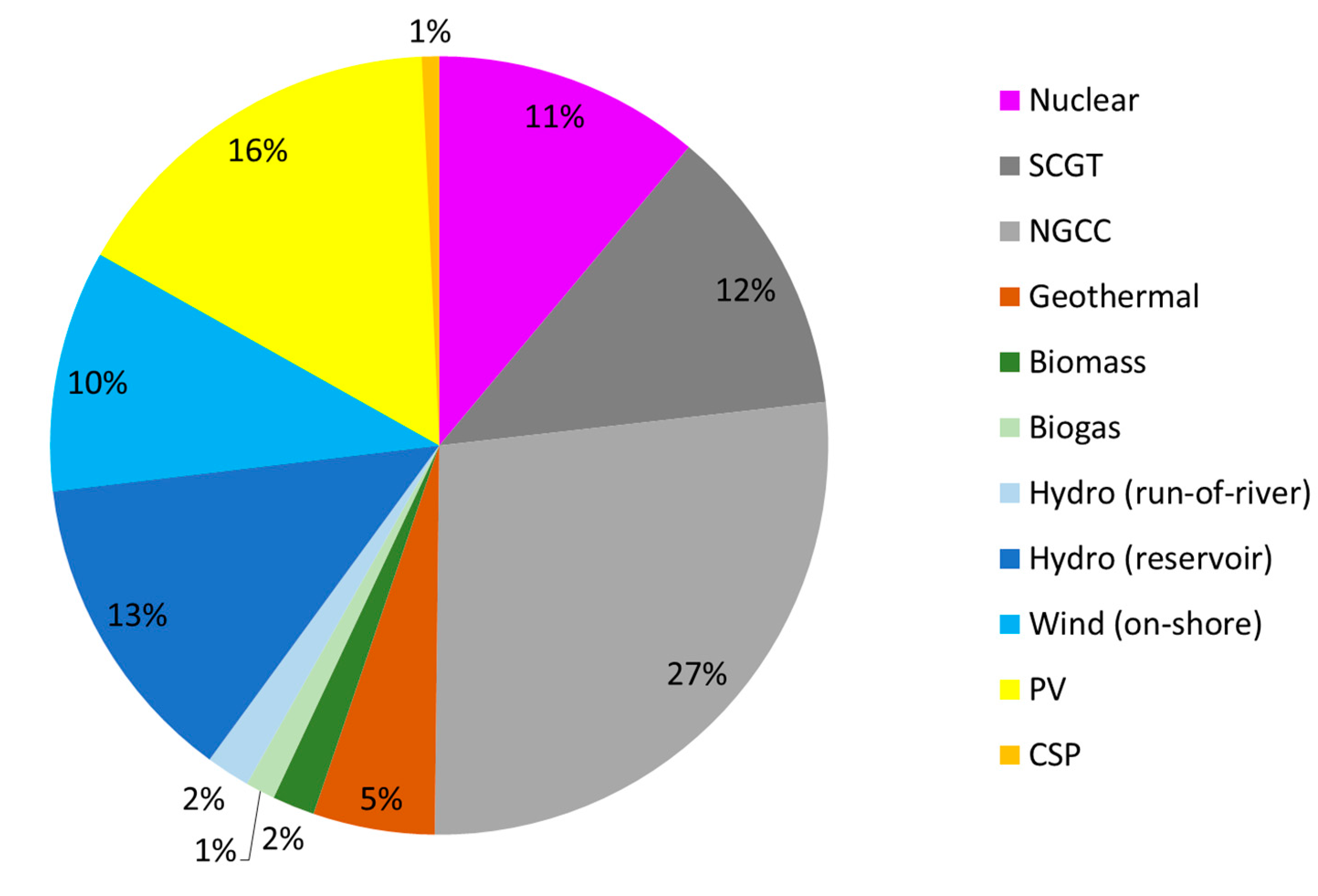
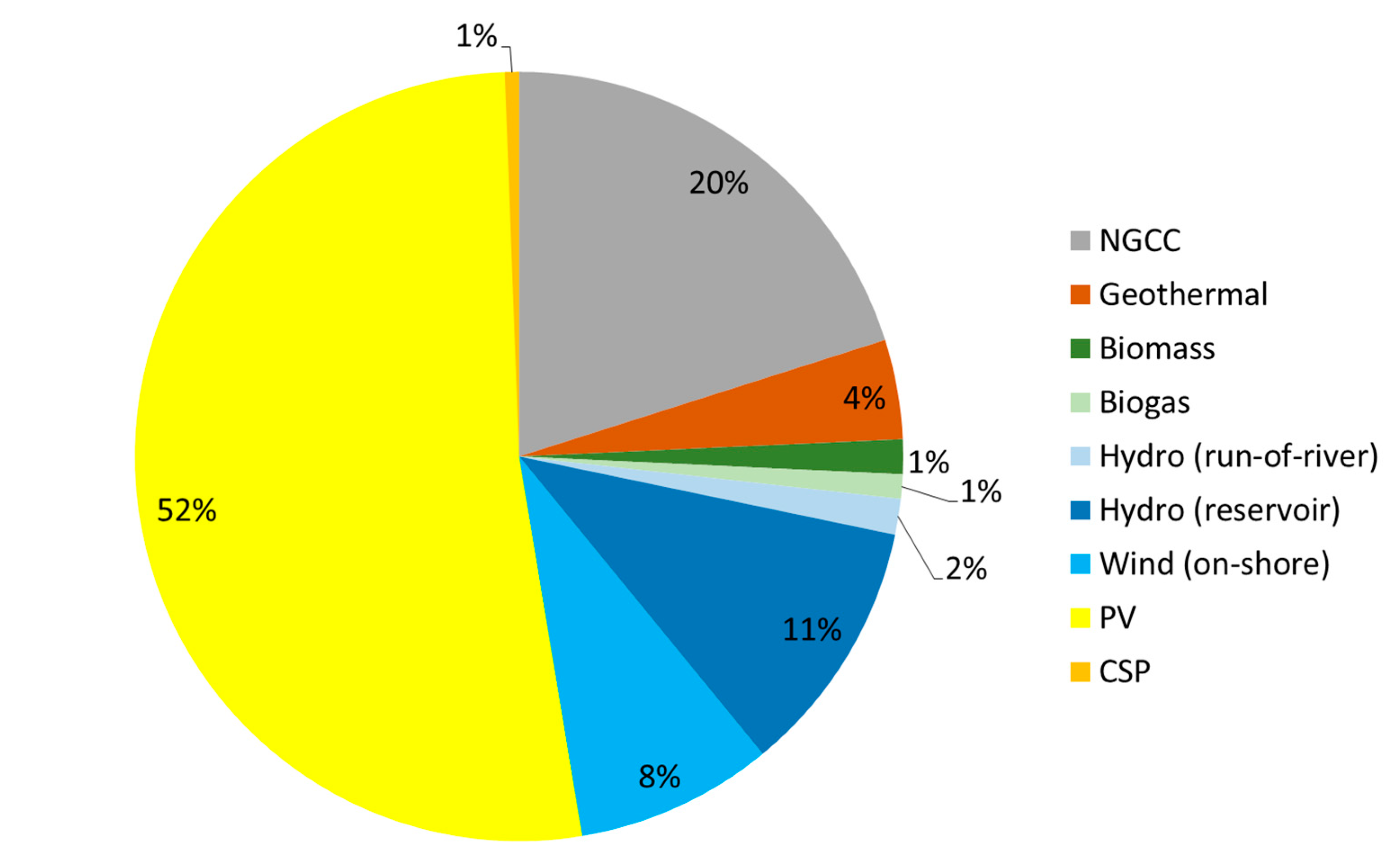
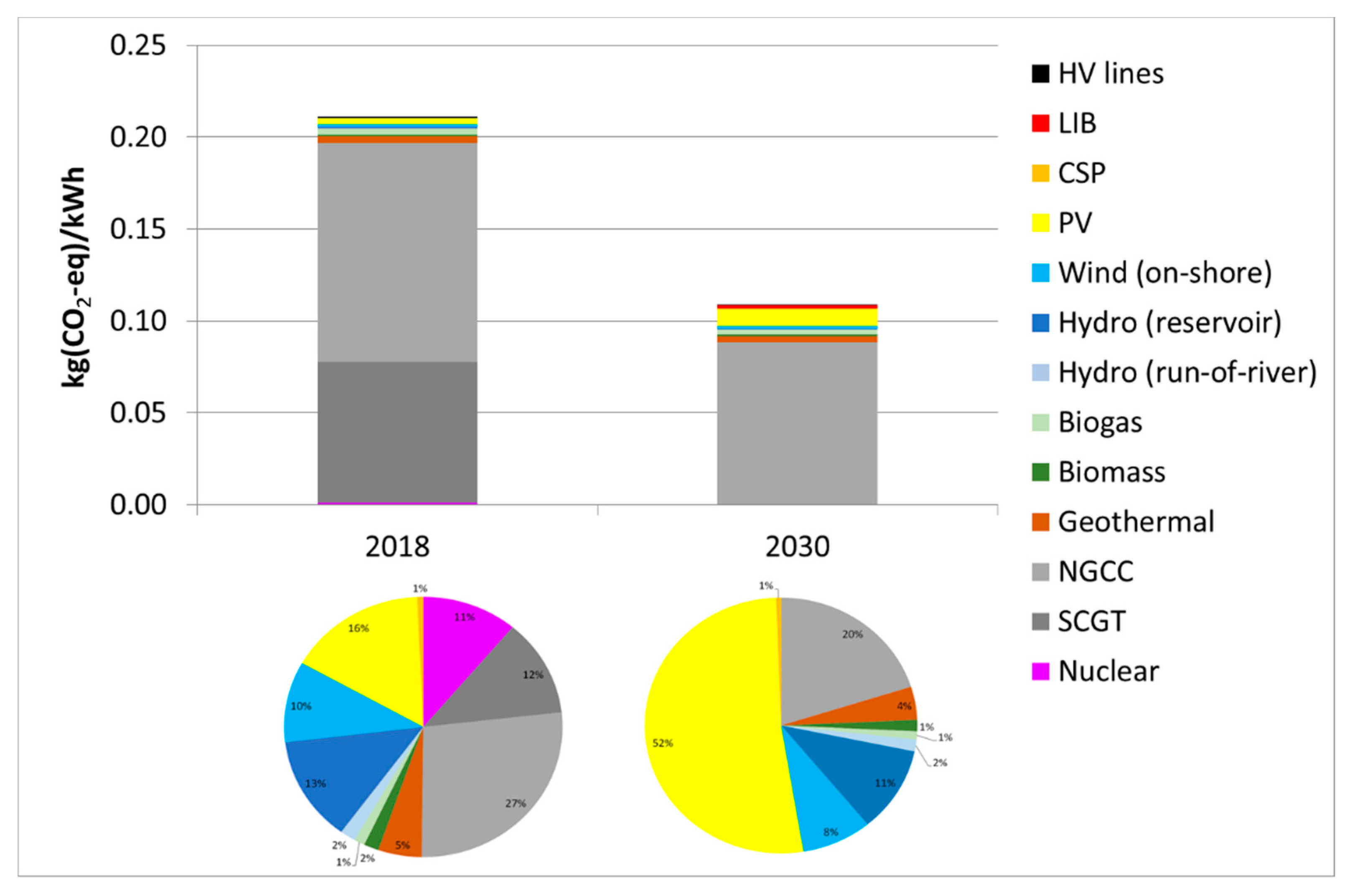
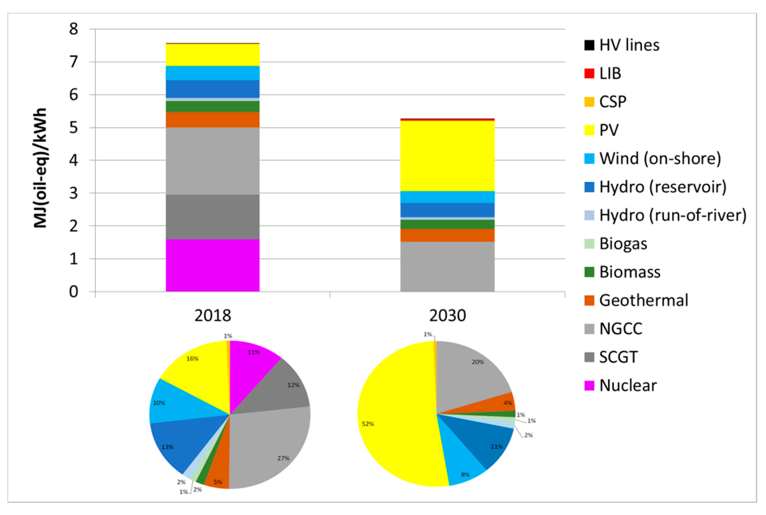
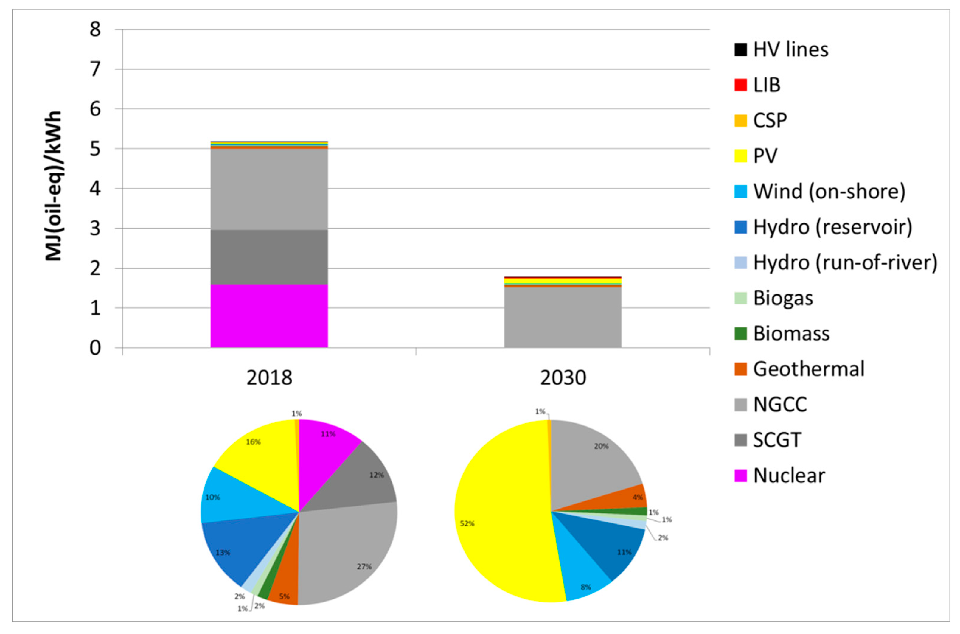
2.3. California Grid Mix Composition in 2018

In 2018 the total California domestic generation was 165 TWh. Figure 1 illustrates the California domestic grid mix composition in terms of total in-state electricity generated in the year 2018. Eleven % of the total in-state electricity was supplied by nuclear reactors, but as explained in Section 2.2.1, all of this is expected to be completely phased out by 2025.
Gas-fired electricity represented 39% of the total in-state generation, but that too is expected to decline due to aggressive California programs to minimize greenhouse gas (GHG) emissions. At the same time, though, it is also expected that gas-fired generation will continue to be a valuable technology for load following, and to compensate for the intermittency of wind and solar generation.
The remaining 50% of the total in-state electricity generation was supplied by RE technologies. Specifically, wind installations generated 10% of the total in-state electricity, while PV systems generated 16% thereof. As discussed in Section 3.1, the share of RE, and specifically PV, is expected to increase significantly over the coming years, with a concomitant surge in the required energy storage capacity.
Finally, electricity transmission was also included within the boundary of this assessment, albeit limited to the high voltage (HV) network. This was deemed an acceptable simplification, since the vast majority of the electricity generation plants comprising the grid mix at present and in the considered future scenario are centralised units which inject HV electricity into the grid. The HV transmission lines were modelled using the WECC-specific life-cycle inventory (LCI) information provided in the Ecoinvent database [38], and transmission losses were set at 6% as per historical data [61].

3. Methods

3.1. Definition of the Future Grid Mix Scenario in 2030

The modelling of the future scenario for the California grid mix in the year 2030 was carried out as described below. Firstly, full hourly-resolution net generation profiles were generated for each technology using the OASIS data collected for 2018 (i.e., the latest available complete datasets at the time of writing). Figure 2 shows the resulting stacked contributions to the total delivered power (black line, which is equal to the demand profile) for a typical day in spring (2nd April). From bottom to top: (I—purple) nuclear (which as expected is almost constant, i.e., a “baseload” provider”), (II—green) other renewables (i.e., the sum of hydro, biogas, biomass and geothermal), (III—blue) wind, (IV—yellow) solar (PV + CSP). Lastly, at any hour, the gap (grey arrow) between the top-most reported generation profile and the demand profile is supplied by a combination of natural gas generation (SCGT + NGCC) and electricity imports.
In addition, the 2018 hourly “potential” PV output was also calculated, by adding back the reported 2018 hourly PV curtailment data to the corresponding net PV generation data. The purpose of this “potential” PV output profile was to provide the basis for the future extrapolation of the corresponding “potential” PV output profile for 2030 (see point 2 below), under the assumption that by then, the large-scale availability of energy storage would negate the need for all technical or economic curtailment other than that due to oversupply (see Section 2.1.3).
Starting from these historical power generation profiles, the corresponding projected profiles for the year 2030 were calculated, based on the modelling assumptions and calculations described below:
(1)
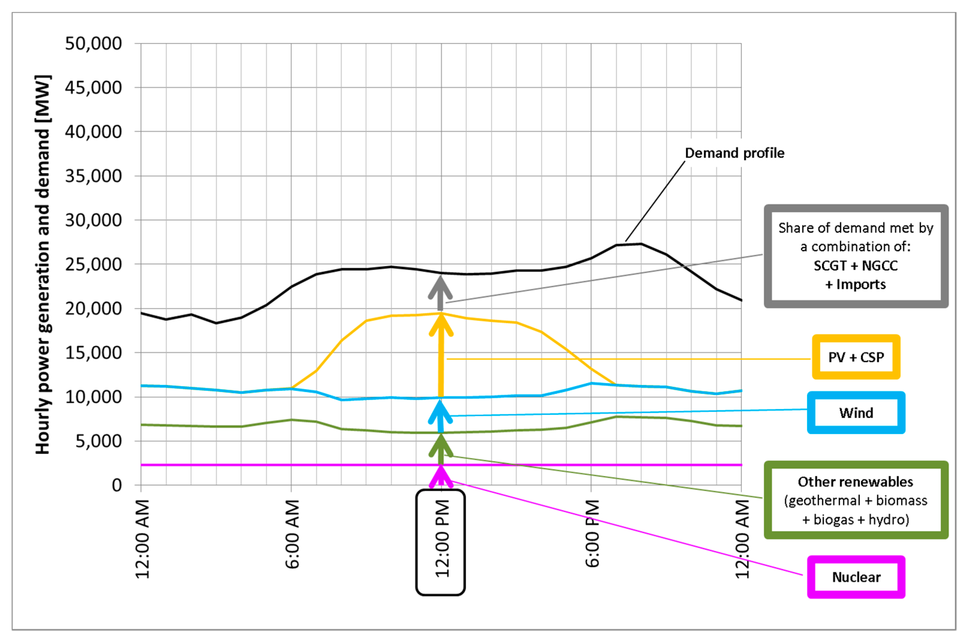
It is assumed that in 2030 the total hourly electricity demand profile will remain the same as in 2018. This future extrapolation is based on the analysis of the demand profiles from 2001 to 2019, which shows that the cumulative yearly electricity demand remained nearly constant during the past 19 years, with minimal oscillations around a centre value of approximately 200 TWh/year. This result appears to be “due to a combination of energy efficiency measures and less electricity-intensive industry that counterbalances increased population and economy” [62]. Other potential variations in electricity demand (both its hourly profile and total year-end cumulative value), for instance due to a possible large-scale deployment of electric vehicles (EVs) and the associated requirement for battery charging, are outside the scope of this study.
(2)
CAISO will rely single-handedly on solar PV as the technology of choice to increase the penetration of renewable energy in the grid. This is a bold assumption, but it was deemed reasonable in view of the abundance of solar irradiation in California, and it also appears to be supported by a simple linear extrapolation of recent past trends, which indicate that wind installations in California have plateaued, whereas PV installations have been sharply and consistently rising (see Figure 3). The final value of installed PV power in 2030 was determined iteratively, so as to match a target of 80% total net domestic renewable electricity generation, after duly taking into account all PV storage and curtailment losses (as explained below). Hence, the PV installed capacity in 2030 is 43,710 MW, as shown in Figure 3. The hourly “potential” (i.e., pre-curtailment and pre-storage) PV output profile was calculated by scaling up the corresponding 2018 “potential” PV electricity generation, proportionally to the respective 2030 vs. 2018 installed power levels.
(3)
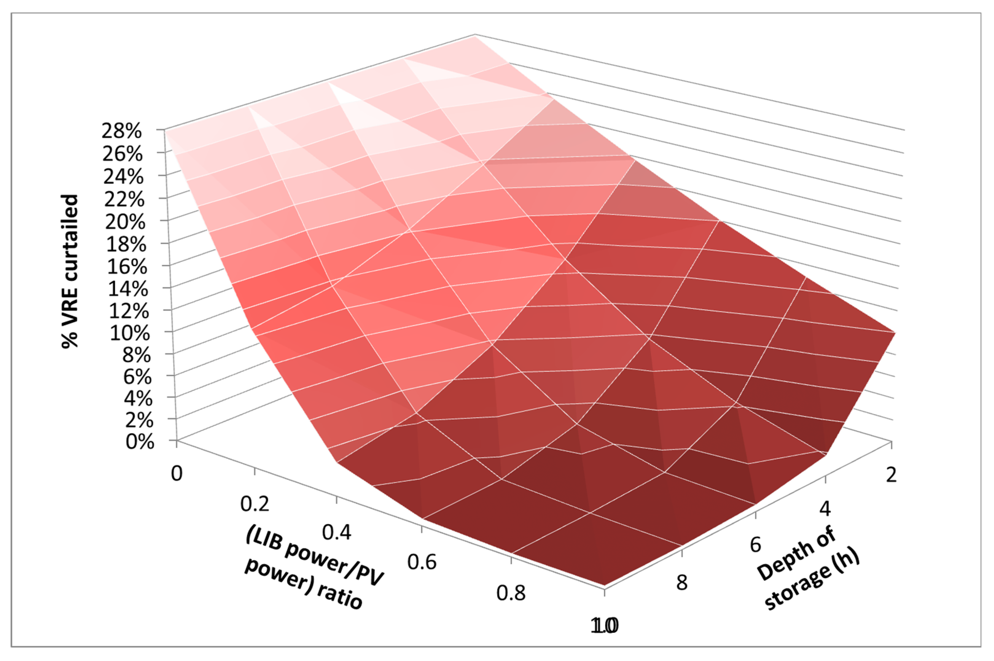
Lithium-ion batteries (LIBs) will be deployed as the storage technology of choice (as discussed in Section 2.2.10). The amount of assumed installed LIB power (P) and the maximum consecutive hours of storage duration at such maximum power (t) were set after performing a parametric investigation of the resulting % of VRE curtailment ensuing from a range of P and t values (following the grid balancing algorithm described at points 7 and 8 below). The results of this parametric analysis are illustrated in Figure 4; in order to make a realistically conservative assumption on the amount of storage, for the purposes of this study the choice was therefore made to set P = 60% of the installed PV power (a value consistent with previous literature [63,64]) and t = 6 h. When taken together, such values of P and t lead to the total installed storage capacity E = P × t. As reported in Table 1, this resulted in 2.8% of the overall “potential” VRE generation being curtailed.
(4)
Nuclear generation will be zero, consistently with the planned decommissioning of all remaining reactors in California (as explained in Section 2.2.1).
(5)
“Other renewables” (i.e., hydro, biogas, biomass and geothermal), wind and CSP generation profiles will remain exactly the same as in 2018.
(6)
Single-cycle gas turbines (SCGT) will be completely phased out.
(7)
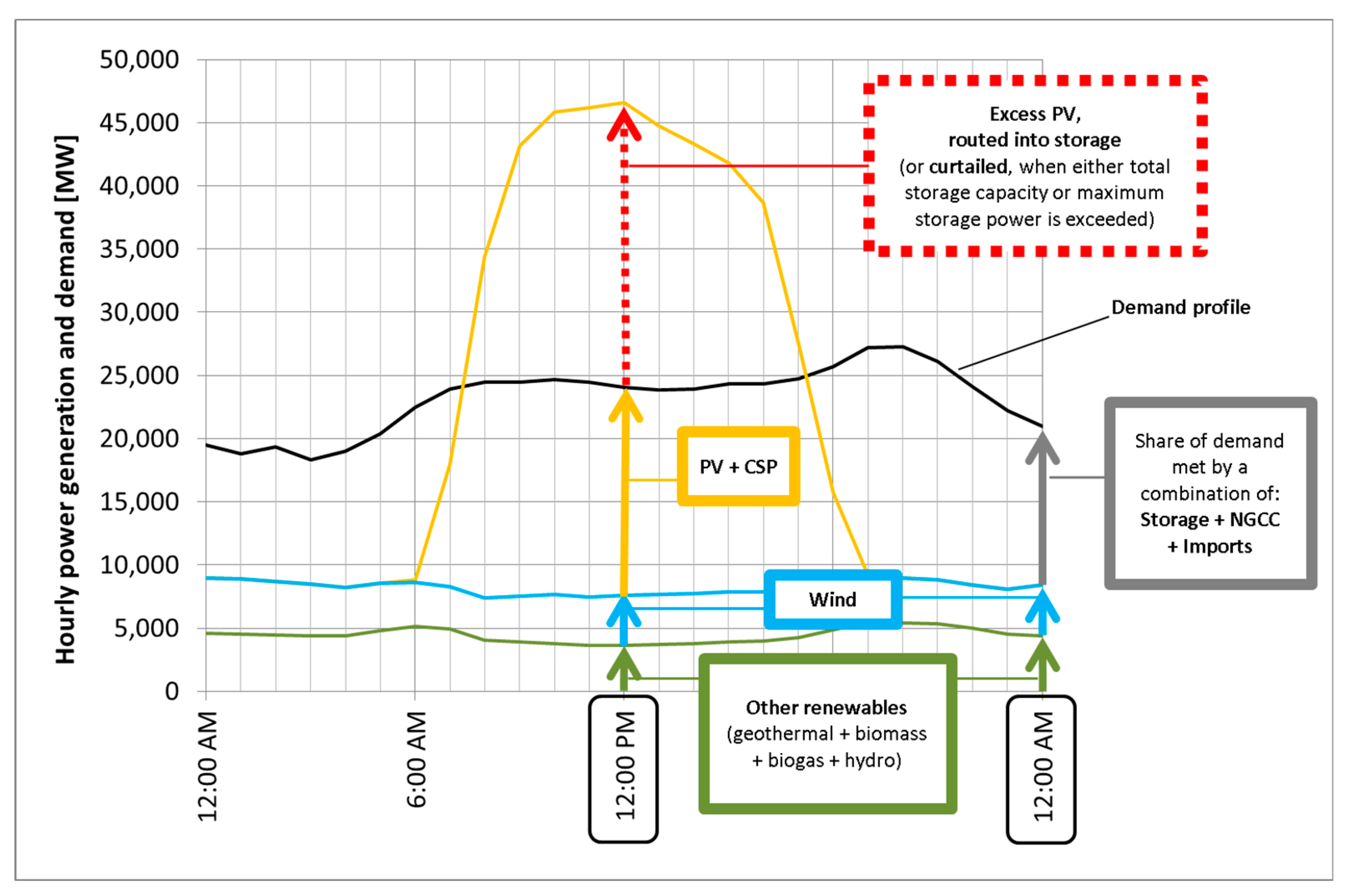
Combined cycle gas turbine (NGCC) output and electricity imports will be used, together with LIB energy storage, to balance overall supply and demand, following a strict order of merit, as follows:
(a)
On an hourly basis, the increased PV output in 2030 with respect to 2018 (more precisely: the difference between the “potential” PV output in 2030, calculated as per point 2 above, and the net PV output in 2018) will first be compensated for by reducing NGCC output. This is deemed the preferred strategy since gas-fired electricity is the most carbon-intensive technology in the California grid mix, and it is also more carbon-intensive than the average mix of technologies used to generate the electricity imported by California [65].
(b)
Then, if/when no residual NGCC power is left, the second intervention will be to curb imported electricity.
(c)
Then, if/when the hourly imported electricity value has been reduced to zero too, and the “potential” PV output is actually in excess of the total demand profile value, such excess PV output will be preferentially routed into storage, as long as neither total storage capacity (E) nor maximum storage power (P) are exceeded.
(d)
Finally, if, after taking steps (a–c) above, either the maximum E or maximum P condition is met, then the residual excess PV output (i.e., the share thereof that cannot be sent to storage) is curtailed.
(8)
After each PV “peak”, i.e., as soon as the “potential” PV profile curve has returned below the total demand profile curve, the electricity stored in LIBs will start being dispatched back to the grid (at a maximum rate limited by P), and will thus curb NGCC output (in the first instance) and imported electricity (if/after NGCC output has already been reduced to zero) with respect to their respective 2018 hourly values.
Figure 5 shows the expected demand profile (black line) for 2 April 2030, and the following stacked power generation profiles, from bottom to top: (I—green) other renewables (hydro + biogas + biomass + geothermal), (II—blue) wind, and (III—yellow) solar (“potential” PV + CSP).
The complete projected hourly electricity generation and demand profiles for the entire year 2030, broken down by month, are reported in the Supplementary Material (Figures S1–S12). Interestingly, because of the large demand for air conditioning in the hotter months in California, the most severe mismatch between the “potential” solar electricity generation and electricity demand profiles occurs in spring, and not in summer, when solar irradiation is highest.
Using the dynamic modelling approach described above, an overall projected year-end domestic grid mix can then be calculated for the California state in 2030. This is illustrated as a pie chart in Figure 6, and its most salient characteristics are compared to those of the corresponding 2018 domestic grid mix in Table 1.
The modelled 2030 California grid mix is characterized by a large share of VRE, out of which 25% is not consumed directly but is instead routed into storage, while only 2.8% is curtailed; the resulting share of net (i.e., post-curtailment and storage) VRE in the domestic grid mix is thus 61%. It is also noteworthy that, even after completely phasing out SCGTs, the remaining required NGCC output is also reduced by 30% (relative to 2018). Also, the hypothesised large deployment of PV + storage yields a surplus of available renewable energy, which, when retrieved from storage, allows a significant reduction in electricity imports, and a corresponding surge in the domestic share of total electricity supply in California, from 73% in 2018 to 88% in 2030.
Lastly, a further interesting finding ensued from a separate sensitivity analysis on the key model assumptions and parameters. While, as mentioned in Section 2.1.1, all nuclear capacity is expected to be phased out in California by the mid-2020s, with no plans for new replacement reactors, it was deemed worthwhile to investigate the theoretical effect that retaining the existing nuclear capacity would have on grid stability, demand for storage and corresponding % VRE curtailment. A first alternative grid model run was then carried out for 2030, with the exact same PV and storage capacities as described above, but in the presence of the same nuclear electricity output as in 2018. This resulted in an increased VRE curtailment rate of 4.3%. Such result was found to be due to the inflexibility of nuclear output, which pushed the “potential” PV output peaks even higher with respect to the demand profile, thereby saturating the available storage capacity sooner. In an alternative model run, the storage duration was then adjusted upwards, so as to increase the total storage capacity and thus bring the % VRE curtailment back down to the same 2.8% as in the “baseline” scenario. This ended up requiring the deployment of 7.3 h of LIB storage vs. 6 h in the “baseline” scenario without nuclear electricity in the mix. The details of this analysis are shown in the Supplementary Material (Table S1 and Figure S13).

3.2. Life Cycle Assessment (LCA)

Life cycle assessment (LCA) is a de-facto standard method for the evaluation of the environmental performance of a wide range of industrial processes and technologies, and it mainly owes its wide acceptance to its comprehensiveness (in terms of considering all supply chain stages, from extraction of raw materials through transportation and manufacturing, to use phase and end-of-life). It also benefits from a high degree of standardization [66,67], and from the availability of extensive, industry-vetted inventory databases, among which a prominent role is played by Ecoinvent [38].
Various life-cycle impact assessment methods have been developed, which enable the calculation of dedicated impact indicators for a wide range of impact categories. Among the latter, the focus of this paper is on global warming potential (GWP), estimated using IPCC-derived characterization factors with a time horizon of 100 years (in units of kg of CO2-equivalent) for all gaseous emissions, excluding biogenic CO2.
Additionally, two life-cycle energy metrics are also calculated here, namely the cumulative energy demand (CED) and the non-renewable cumulative energy demand (nr-CED), respectively quantifying the total amount of primary energy directly and indirectly harvested from the environment per unit of electricity output, and the non-renewable share thereof (in both cases the results are expressed in MJ of oil-equivalent) [68].
Based on the definition above, it is also self-evident that the life-cycle primary-to-electric energy conversion efficiency of the grid mix taken as a whole (ηG) can be conveniently calculated as the reciprocal of its CED (Equation (1)):
ηG = 1/CEDG

3.3. Net Energy Analysis (NEA)

Net energy analysis (NEA) [69] provides an alternative viewpoint on the energy metabolism of energy harvesting and conversion technologies, whereby the primary energy resource(s) that are directly exploited and converted to useful energy carriers (e.g., the natural gas that is extracted, conveyed by pipeline and then burnt in a power plant to produce electricity; or the solar energy that is harvested and converted to electricity by PV panels) are deliberately excluded from the accounting, and instead the focus is put solely on how much previously-available commercial energy needs to be “invested” in order to operate the energy supply chains (e.g., the energy needed to extract the gas from the ground, build the pipeline, pump the gas through the pipeline, and build the gas turbine; or the energy needed to manufacture the PV panels and their balance-of-system).
When put in rather blunt but arguably vivid terms, it can therefore be said that instead of being concerned with the overall thermodynamic efficiency of a process, NEA aims to quantify the energy “bang for the buck” from the point of view of the end user. Fittingly, its main indicator is the energy return on (energy) investment [70] (defined as per Equation (2)):
EROI = Out/Inv
However, the NEA literature has historically been characterized by a much lower degree of standardization than the LCA one, which has led to many inconsistent comparisons [71,72].
In this study, in order to integrate the LCA and NEA viewpoints, and to maximize the consistency of the calculations, both internally and externally with some of the more recent literature [10,12,13,15,17], when calculating the EROI of electricity (either produced by a specific technology, or by the grid mix as a whole), all energy investments at the denominator are always accounted for in terms of their respective life-cycle CED (and are thus quantified in units of oil-equivalent).
Then, when the EROI numerator is simply measured as the amount of electricity delivered (i.e., not converted to some form of “equivalent” primary or thermal energy), a subscript “el” is appended to the resulting indicator (i.e., EROIel). Alternatively, when the EROI numerator is expressed as “primary energy equivalent” (on the basis of the life-cycle primary-to-electric energy conversion efficiency of the grid mix in the current year), a subscript “PE-eq” is used (i.e., EROIPE-eq).

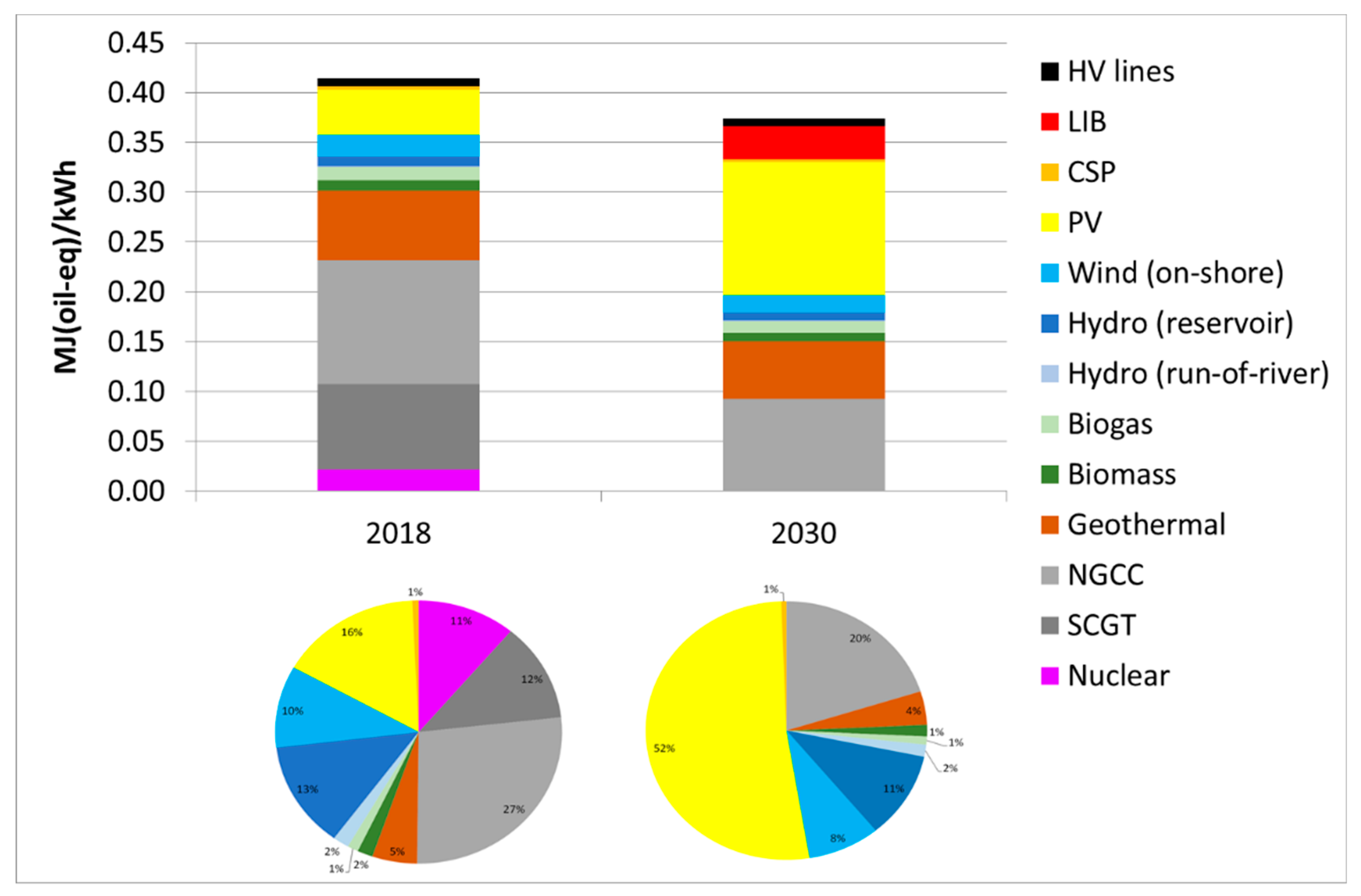
4. Results and Discussion

Figure 7 illustrates the calculated GWP of the domestic grid mix in California, respectively in 2018 (based on historical data) and in 2030 (when the future grid mix is modelled as described in Section 3.1). The first and foremost result is that the carbon intensity of electricity is expected to be almost halved over the course of a single decade. Such remarkable drop is almost entirely due to the combination of two key factors. Firstly, the massive deployment of PV and energy storage allows a substantial phasing out of gas-fired electricity (and SCGTs in particular). Secondly, the up-front carbon emissions due to the manufacturing and installation of the PV and LIB systems are low enough that, when discounted over the total amount of electricity that they deliver in their combined service lives, they result in comparatively negligible GWP contributions to the grid mix.
These results are put in even starker relief when considering that in 2018, gas-fired power plants generated 29% of total domestic electricity while being responsible for 93% of the grid’s GWP; conversely, in 2030 PV + LIBs are expected to generate 52% of total domestic electricity while only causing 10% of the grid’s total carbon emissions.
In terms of life-cycle energy results, the same planned energy transition results in an overall 31% reduction in the CED of domestic electricity in California (Figure 8), and a corresponding increase in the life-cycle primary-to-electric energy conversion efficiency (ηG) of the grid mix, from 48% to 69%.
The improvement becomes even more significant when specifically focusing on the life-cycle demand for non-renewable primary energy (Figure 9), given that most of the primary energy harvested from the environment to power the grid mix in 2030 is actually renewable (i.e., solar, and to a lesser extent wind, hydro, geothermal and biomass).
As a result, the nr-CED of domestic electricity in California drops by a factor of three, from 5.2 to 1.8 MJ(oil-eq)/kWh. To this effect, it is noteworthy that phasing out nuclear, as well as natural gas, is also beneficial (while nuclear energy is a low-carbon technology, it still obviously relies on non-renewable stocks of fissile fuel, which are also not available domestically in California, adding further meaning to these results in terms of improved energy sovereignty).
Finally, when shifting the viewpoint to the one characteristic of NEA, and thus focusing only on the energy investment per unit of electricity delivered, while excluding the primary energy that is directly harvested and converted to electricity, Figure 10 shows that the planned massive deployment of PV and LIB storage in 2030 does result in significant shares of the total grid mix energy investment being required for these technologies (respectively, 36% and 9%). Even so, the overall energy investment per unit of delivered electricity in 2030 is still reduced with respect to the historical value for 2018.
As illustrated in Figure 11, this results in a 10% increase in the EROIel of the California domestic grid mix as a whole. At the same time, however, because of the larger penetration of PV and the phasing out of nuclear and, partially, gas-fired electricity, the life-cycle primary-to-electric energy conversion efficiency of the grid mix (ηG) increases by as much as 44% in relative terms, from ηG = 0.48 in 2018 to ηG = 0.69 in 2030. Therefore, the trend in EROIPE-eq = EROIelG ends up being dominated by the latter change in ηG.
In order to provide additional detail on these NEA calculations, the specific EROI results (in terms of both electricity and equivalent primary energy) for the individual electricity generation technologies comprising the California domestic grid mix in 2018 and 2030 are reported in Table 2. Once again, it is noteworthy that the ηG values for California in 2018 and 2030 are significantly higher than typically assumed for electricity grids with higher percentages of thermal technologies (ηG = 0.30–0.35), resulting in comparatively lower values of EROIPE-eq. This showcases how any specific EROIPE-eq values are only valid for the actual conditions considered in each study (such as grid mix composition, year, and location).
Specifically, changes in ηG are at the root of the differences in EROIPE-eq results for PV in California vs. those previously reported by the same authors when considering a more generalised thermal grid mix (ηG = 0.30) [50].
Finally, by way of sensitivity analysis, an alternative scenario for 2030 was also analysed, in which more efficient and longer-lasting PV systems were assumed (cf. Section 2.2.9). The ensuing variations in the calculated energy and carbon emission indicators for the California domestic grid mix are reported in Table 3. As can be seen, this sensitivity analysis proves that the main results of this study are very robust and not likely to be affected significantly by alternative future PV developments.

5. Conclusions

This analysis has shown that an energy transition in the California electricity sector hinging on the large-scale deployment of photovoltaic energy with lithium-ion battery energy storage (with a concomitant reduction in gas-fired electricity generation) would potentially be very effective at swiftly curbing GHG emissions, down to one half of the current level by 2030.
The non-renewable primary energy requirement per unit of electricity delivered could also be reduced by a factor of three, with benefits in terms of sustainability and positive implications in terms of domestic energy sovereignty.
Importantly, from the point of view of net energy delivery, contrary to previously voiced concerns, this analysis has also found that the overall energy return on energy investment (EROI) of a future electricity grid mix largely dependent on variable renewable energy plus storage does not have to suffer with respect to a current mix more heavily reliant on conventional thermal technologies such as nuclear and gas.
Additionally, the planned complete phasing out of nuclear energy in California does not appear to be detrimental to the future energy performance of the state’s domestic grid, even when fully taking into account the mismatch between the hourly electricity demand and variable renewable energy resource availability profiles.
A degree of uncertainty remains on the future technological improvement trajectories for PV and battery technologies; however, all the aforementioned broadly positive results were produced when making rather conservative assumptions in both regard; further, a sensitivity analysis on future PV efficiencies and lifetimes has confirmed the robustness of the results.
A further source of uncertainty for the future is the possible change in electricity demand (both in terms of its hourly profile, and of the total year-end cumulative value) that could be brought about by a massive deployment of electric vehicles (EVs), with the associated requirement for battery charging. At the same time, though, a large EV fleet could also reduce the requirement for dedicated grid-level energy storage, by providing some of the required storage capacity through vehicle-to-grid (V2G) schemes. Accurately modelling the combined effects caused by these sector-wide changes was outside the scope of this paper but provides scope for future related research.
Future studies are also needed to address other potential environmental impacts in categories such as metal resource depletion and human and ecological toxicity. However, these types of impact are much harder to quantify, due to current uncertainties on emissions from mining activities [73], a range of methodological challenges, both in terms of characterization [74,75,76,77], and of the required but often delicate and difficult assumptions in terms of allocation [78].

Supplementary Materials

The following are available online at https://www.mdpi.com/1996-1073/13/15/3934/s1, Figures S1–S12: Complete projected hourly electricity generation and demand profiles for the entire year 2030, broken down by month. Table S1 and Figure S13: Sensitivity analysis on the % VRE curtailment, resulting from alternative nuclear and storage deployment hypotheses in 2030.

Author Contributions

Conceptualization, M.R.; methodology, M.R.; software, M.R., A.P. and E.L.; validation, M.R., E.L. and V.F.; formal analysis, M.R.; investigation, M.R. and A.P.; resources, M.R. and A.P.; data curation, M.R., E.L. and A.P.; writing—original draft preparation, M.R., A.P. and E.L.; writing—review and editing, M.R. and V.F.; visualization, M.R., A.P. and E.L.; supervision, M.R. and V.F. All authors have read and agreed to the published version of the manuscript.

Funding

This work was supported in part by the Faraday Institution [grant number FIR005].

Conflicts of Interest

The authors declare no conflict of interest.

References

  1. Ritchie, H.; Roser, M. CO2 and Greenhouse Gas Emissions. Our World in Data. Available online: https://ourworldindata.org/co2-and-other-greenhouse-gas-emissions#global-warming-to-date (accessed on 19 June 2020).
  2. Dejuán, Ó.; Lenzen, M.; Cadarso, M.Á. (Eds.) Environmental and Economic Impacts of Decarbonization: Input-Output Studies on the Consequences of the 2015 Paris Agreements, 1st ed.; Routledge: Abingdon, UK, 2018; p. 402. [Google Scholar]
  3. Sørensen, B. Energy and resources. Science 1975, 189, 255–260. [Google Scholar] [CrossRef] [PubMed]
  4. Lovins, A.B. Energy strategy: The road not taken. Foreign Aff. 1976, 55, 636–640. [Google Scholar] [CrossRef]
  5. Sørensen, B.; Meibom, P. A global renewable energy scenario. Int. J. Glob. Energy Issues 2000, 13, 196–276. [Google Scholar] [CrossRef]
  6. Fthenakis, V.; Mason, J.E.; Zweibel, K. The technical, geographical, and economic feasibility for solar energy to supply the energy needs of the US. Energy Policy 2009, 37, 387–399. [Google Scholar] [CrossRef]
  7. Jacobson, M.Z.; Delucchi, M.A.; Cameron, M.A.; Mathiesen, B.V. Matching demand with supply at low cost in 139 countries among 20 world regions with 100% intermittent wind, water, and sunlight (WWS) for all purposes. Renew. Energy 2018, 123, 236–248. [Google Scholar] [CrossRef]
  8. Brown, T.W.; Bischof-Niemz, T.; Blok, K.; Breyer, C.; Lund, H.; Mathiesen, B.V. Response to ‘Burden of proof: A comprehensive review of the feasibility of 100% renewable-electricity systems’. Renew. Sust. Energy Rev. 2018, 92, 834–847. [Google Scholar] [CrossRef]
  9. Diesendorf, M.; Elliston, B. The feasibility of 100% renewable electricity systems: A response to critics. Renew. Sust. Energy Rev. 2018, 93, 318–330. [Google Scholar] [CrossRef]
  10. Raugei, M.; Leccisi, E. A comprehensive assessment of the energy performance of the full range of electricity generation technologies deployed in the United Kingdom. Energy Policy 2016, 90, 46–59. [Google Scholar] [CrossRef] [Green Version]
  11. Jones, C.; Gilbert, P.; Raugei, M.; Leccisi, E.; Mander, S. An Approach to Prospective Consequential LCA and Net Energy Analysis of Distributed Electricity Generation. Energy Policy 2017, 100, 350–358. [Google Scholar] [CrossRef]
  12. Raugei, M.; Leccisi, E.; Azzopardi, B.; Jones, C.; Gilbert, P.; Zhang, L.; Zhou, Y.; Mander, S.; Mancarella, P. A multi-disciplinary analysis of UK grid mix scenarios with large-scale PV deployment. Energy Policy 2018, 114, 51–62. [Google Scholar] [CrossRef]
  13. Raugei, M.; Leccisi, E.; Fthenakis, V.; Moragas, R.E.; Simsek, Y. Net energy analysis and life cycle energy assessment of electricity supply in Chile: Present status and future scenarios. Energy 2018, 162, 659–668. [Google Scholar] [CrossRef] [Green Version]
  14. Leccisi, E.; Raugei, M.; Fthenakis, V. The energy performance of potential scenarios with large-scale PV deployment in Chile a dynamic analysis 2018. In Proceedings of the IEEE 7th World Conference on Photovoltaic Energy Conversion (WCPEC), Waikoloa Village, HI, USA, 10–15 June 2018; pp. 2441–2446. [Google Scholar]
  15. Murphy, D.J.; Raugei, M. The Energy Transition in New York: A Greenhouse Gas, Net Energy and Life-Cycle Energy Analysis. Energy Technol. 2020. [Google Scholar] [CrossRef]
  16. Osorio-Aravena, J.C.; Aghahosseini, A.; Bogdanov, D.; Caldera, U.; Muñoz-Cerón, E.; Breyer, C. Transition toward a fully renewable based energy system in Chile by 2050 across power, heat, transport and desalination sectors. Int. J. Sustain. Energy Plan. Manag. 2020, 25, 77–94. [Google Scholar]
  17. Raugei, M.; Kamran, M.; Hutchinson, M. A Prospective Net Energy and Environmental Life-Cycle Assessment of the UK Electricity Grid. Energies 2020, 13, 2207. [Google Scholar] [CrossRef]
  18. California State. Senate Bill No. 100 Chapter 312. An Act to amend Sections 399.11, 399.15, and 399.30 of, and to Add Section 454.53 to, the Public Utilities Code, Relating to Energy. 2018. Available online: https://leginfo.legislature.ca.gov/faces/billTextClient.xhtml?bill_id=201720180SB100 (accessed on 19 June 2020).
  19. Haegel, N.M.; Atwater, H.; Barnes, T.; Breyer, C.; Burrell, A.; Chiang, Y.M.; De Wolf, S.; Dimmler, B.; Feldman, D.; Glunz, S.; et al. Terawatt-scale photovoltaics: Transform global energy. Science 2019, 364, 836–838. [Google Scholar] [CrossRef] [PubMed] [Green Version]
  20. Arbabzadeh, M.; Sioshansi, R.; Johnson, J.X.; Keoleian, G.A. The role of energy storage in deep decarbonization of electricity production. Nat. Commun. 2019, 10, 1–11. [Google Scholar] [CrossRef] [Green Version]
  21. Comello, S.; Reichelstein, S. The emergence of cost effective battery storage. Nat. Commun. 2019, 10, 1–9. [Google Scholar] [CrossRef] [Green Version]
  22. Cebulla, F.; Haas, J.; Eichman, J.; Nowak, W.; Mancarella, P. How much electrical energy storage do we need? A synthesis for the US, Europe, and Germany. J. Clean. Prod. 2018, 181, 449–459. [Google Scholar] [CrossRef]
  23. Denholm, P.; Margolis, R. Energy Storage Requirements for Achieving 50% Solar Photovoltaic Energy Penetration in California. National Renewable Energy Laboratory 2016. NREL/TP-6A20-66595. Available online: https://www.nrel.gov/docs/fy16osti/66595.pdf (accessed on 19 June 2020).
  24. California ISO. Renewable Grid Initiative. Energy Storage. Perspectives from California and Europe 2019. Available online: http://www.caiso.com/Documents/EnergyStorage-PerspectivesFromCalifornia-Europe.pdf (accessed on 19 June 2020).
  25. Wadia, C.; Albertus, P.; Srinivasan, V. Resource constraints on the battery energy storage potential for grid and transportation applications. J. Power Sources 2011, 196, 1593–1598. [Google Scholar] [CrossRef] [Green Version]
  26. Roy, S.; Sinha, P.; Shah, S.I. Assessing the Techno-Economics and Environmental Attributes of Utility-Scale PV with Battery Energy Storage Systems (PVS) Compared to Conventional Gas Peakers for Providing Firm Capacity in California. Energies 2020, 13, 488. [Google Scholar] [CrossRef] [Green Version]
  27. Pellow, M.A.; Ambrose, H.; Mulvaney, D.; Betita, R.; Shaw, S. Research gaps in environmental life cycle assessments of lithium ion batteries for grid-scale stationary energy storage systems: End-of-life options and other issues. SMT 2020, 23, 00120. [Google Scholar] [CrossRef]
  28. Raugei, M.; Leccisi, E.; Fthenakis, V.M. What Are the Energy and Environmental Impacts of Adding Battery Storage to Photovoltaics? A Generalized Life Cycle Assessment. Energy Technol. 2020. [Google Scholar] [CrossRef]
  29. Diesendorf, M.; Wiedmann, T. Implications of trends in energy return on energy invested (EROI) for transitioning to renewable electricity. Ecol. Econ. 2020, 176, 106726. [Google Scholar] [CrossRef]
  30. California ISO 2013. Demand Response and Energy Efficiency Roadmap: Maximizing Preferred Resources. Available online: https://www.caiso.com/Documents/DR-EERoadmap.pdf (accessed on 19 June 2020).
  31. California ISO. Available online: http://www.caiso.com/about/Pages/default.aspx (accessed on 19 June 2020).
  32. Congress. Gov. Available online: https://www.congress.gov/bill/102nd-congress/house-bill/776?q=%7B%22search%22%3A%5B%22H.R.776.ENR%22%5D%7D&s=8&r=7 (accessed on 19 June 2020).
  33. Federal Energy Regulatory Commission. Available online: https://www.ferc.gov/legal/maj-ord-reg/land-docs/order888.asp (accessed on 19 June 2020).
  34. Federal Energy Regulatory Commission. Available online: https://www.ferc.gov/legal/maj-ord-reg/land-docs/order889.asp (accessed on 19 June 2020).
  35. California ISO. Available online: https://www.caiso.com/TodaysOutlook/Pages/default.aspx (accessed on 19 June 2020).
  36. California Energy Commission. Electric Generation Capacity and Energy. Available online: https://www.energy.ca.gov/data-reports/energy-almanac/california-electricity-data/electric-generation-capacity-and-energy (accessed on 15 July 2020).
  37. California Energy Commission. Available online: https://www.energy.ca.gov/data-reports/california-power-generation-and-power-sources/nuclear-energy (accessed on 19 June 2020).
  38. Ecoinvent Life Cycle Inventory Database. 2019. Available online: https://www.ecoinvent.org/database/database.html (accessed on 19 June 2020).
  39. Pacific Gas and Electric Company. Available online: https://www.pge.com/en_US/safety/how-the-system-works/diablo-canyon-power-plant/diablo-canyon-power-plant.page (accessed on 19 June 2020).
  40. Nyberg, M. Thermal Efficiency of Gas-Fired Generation in California: 2016 Update. California Energy Commission. CEC 200-2017-003; 2017. Available online: https://ww2.energy.ca.gov/2017publications/CEC-200-2017-003/CEC-200-2017-003.pdf (accessed on 19 June 2020).
  41. Southern California Gas Company. Available online: https://www.socalgas.com/regulatory/cgr (accessed on 19 June 2020).
  42. California Energy Commission. Available online: https://ww2.energy.ca.gov/almanac/renewables_data/biomass/index_cms.php (accessed on 19 June 2020).
  43. California Energy Commission. Available online: https://ww2.energy.ca.gov/biomass/anaerobic.html (accessed on 19 June 2020).
  44. US Geological Survey. Available online: https://emp.lbl.gov/publications/us-wind-turbine-database-files (accessed on 19 June 2020).
  45. National Renewable Energy Laboratory (NREL). Available online: https://solarpaces.nrel.gov/by-country/US (accessed on 19 June 2020).
  46. Moreno-Ruiz, E.; Valsasina, L.; FitzGerald, D.; Brunner, F.; Symeonidis, A.; Bourgault, G.; Wernet, G. Documentation of Changes Implemented in Ecoinvent Database v3.6; Ecoinvent Association: Zürich, Switzerland, 2019. [Google Scholar]
  47. Burkhardt, J.; Heath, G.; Turchi, C. Life cycle assessment of a parabolic trough concentrating solar power plant and the impacts of key design alternatives. Environ. Sci. Technol. 2011, 45, 2457–2464. [Google Scholar] [CrossRef] [PubMed]
  48. Whitaker, M.B.; Heath, G.A.; Burkhardt, J.J., III; Turchi, C.S. Life cycle assessment of a power tower concentrating solar plant and the impacts of key design alternatives. Environ. Sci. Technol. 2013, 47, 5896–5903. [Google Scholar] [CrossRef]
  49. Photovoltaics Report. Fraunhofer Institute for Solar Energy Systems. 2019. Available online: https://www.ise.fraunhofer.de/en/publications/studies/photovoltaics-report.html (accessed on 20 March 2020).
  50. Leccisi, E.; Raugei, M.; Fthenakis, V. The energy and environmental performance of ground-mounted photovoltaic systems—A timely update. Energies 2016, 9, 622. [Google Scholar] [CrossRef] [Green Version]
  51. Frischknecht, R.; Itten, R.; Sinha, P.; De Wild-Scholten, M.; Zhang, J.; Fthenakis, V.; Kim, H.C.; Raugei, M.; Stucki, M. Life Cycle Inventories and Life Cycle Assessment of Photovoltaic Systems; Report IEA-PVPS T12-04:2015; International Energy Agency (IEA): Paris, France, 2015. [Google Scholar]
  52. Corcelli, F.; Ripa, M.; Leccisi, E.; Cigolotti, V.; Fiandra, V.; Graditi, G.; Sannino, L.; Tammaro, M.; Ulgiati, S. Sustainable urban electricity supply chain—Indicators of material recovery and energy savings from crystalline silicon photovoltaic panels end-of-life. Ecol. Indic. 2016, 94, 37–51. [Google Scholar] [CrossRef] [Green Version]
  53. Frischknecht, R.; Itten, R.; Wyss, F.; Blanc, I.; Heath, G.; Raugei, M.; Sinha, P.; Wade, A. Life Cycle Assessment of Future Photovoltaic Electricity Production from Residential-Scale Systems Operated in Europe; Report T12-05:2015; International Energy Agency: Paris, France, 2015; Available online: http://www.iea-pvps.org (accessed on 19 June 2020).
  54. Leccisi, E.; Fthenakis, V. Life-cycle environmental impacts of single-junction and tandem perovskite PVs: A critical review and future perspectives. Prog. Energy 2020, in press. [Google Scholar] [CrossRef]
  55. Palizban, O.; Kauhaniemi, K. Energy storage systems in modern grids—Matrix of technologies and applications. J. Energy Storage 2016, 6, 248–259. [Google Scholar] [CrossRef]
  56. IRENA. Electricity Storage and Renewables: Costs and Markets to 2030; International Renewable Energy Agency: Abu Dhabi, UAE, 2017. Available online: https://www.irena.org/publications/2017/Oct/Electricity-storage-and-renewables-costs-and-markets (accessed on 19 June 2020).
  57. Lindley, D. Smart grids: The energy storage problem. Nature 2010, 463, 18–20. [Google Scholar] [CrossRef] [Green Version]
  58. Blakers, A.; Lu, B.; Stocks, M. 100% renewable electricity in Australia. Energy 2017, 133, 471–482. [Google Scholar] [CrossRef]
  59. Center for Sustainable Systems. U.S. Energy Storage Factsheet; Pub. No. CSS15-17. University of Michigan: Ann Arbor, MI, USA, 2018. Available online: http://css.umich.edu/factsheets/us-grid-energy-storage-factsheet (accessed on 19 June 2020).
  60. Xu, B.; Oudalov, A.; Ulbig, A.; Andersson, G.; Kirschen, D.S. Transactions on Smart Grid. IEEE 2016, 9, 1131–1140. [Google Scholar]
  61. Wong, L. A Review of Transmission Losses in Planning Studies: Staff Paper; California Energy Commission: Sacramento, CA, USA, 2011. [Google Scholar]
  62. Colbertaldo, P.; Agustin, S.B.; Campanari, S.; Brouwer, J. Impact of hydrogen energy storage on California electric power system: Towards 100% renewable electricity. Int. J. Hydrogen Energy 2019, 44, 9558–9576. [Google Scholar] [CrossRef]
  63. Fu, R.; Remo, T.; Margolis, R. 2018 U.S. Utility-Scale Photovoltaics-Plus-Energy Storage System Costs Benchmark; Report NREL/TP-6A20-71714; National Renewable Energy Laboratory: Golden, CO, USA, 2018. Available online: https://www.nrel.gov/docs/fy19osti/71714.pdf (accessed on 19 June 2020).
  64. Denholm, P.; Eichman, J.; Margolis, R. Evaluating the Technical and Economic Performance of PV Plus Storage Power Plants; Report NREL/TP-6A20-68737; National Renewable Energy Laboratory: Golden, CO, USA, 2017. Available online: https://www.nrel.gov/docs/fy17osti/68737.pdf (accessed on 19 June 2020).
  65. California Energy Commission. 2018 Total System Electric Generation. Available online: https://www.energy.ca.gov/data-reports/energy-almanac/california-electricity-data/2018-total-system-electric-generation (accessed on 19 June 2020).
  66. Environmental Management. Life Cycle Assessment. Principles and Framework. Standard ISO 14040; International Organization for Standardization: Geneva, Switzerland, 2006; Available online: https://www.iso.org/standard/37456.html (accessed on 27 March 2020).
  67. Environmental Management. Life Cycle Assessment. Principles and Framework. Standard ISO 14044; International Organization for Standardization: Geneva, Switzerland, 2006; Available online: https://www.iso.org/standard/38498.html (accessed on 27 March 2020).
  68. Frischknecht, R.; Wyss, F.; Büsser Knöpfel, S.; Lützkendorf, T.; Balouktsi, M. Cumulative energy demand in LCA: The energy harvested approach. Int. J. Life Cycle ASS 2015, 20, 957–969. [Google Scholar] [CrossRef]
  69. Carbajales-Dale, M.; Barnhart, C.; Brandt, A.; Benson, S. A better currency for investing in a sustainable future. Nat. Clim. Chang. 2014, 4, 524–527. [Google Scholar] [CrossRef]
  70. Hall, C.; Lavine, M.; Sloane, J. Efficiency of Energy Delivery Systems: I. an Economic and Energy Analysis. Environ. Manag. 1979, 3, 493–504. [Google Scholar] [CrossRef]
  71. Murphy, D.J.; Carbajales-Dale, M.; Moeller, D. Comparing Apples to Apples: Why the Net Energy Analysis Community Needs to Adopt the Life-Cycle Analysis Framework. Energies 2016, 9, 917. [Google Scholar] [CrossRef]
  72. Raugei, M. Net Energy Analysis must not compare apples and oranges. Nat. Energy 2019, 4, 86–88. [Google Scholar] [CrossRef]
  73. Classen, M.; Althaus, H.-J.; Blaser, S.; Doka, G.; Jungbluth, N.; Tuchschmid, M. Life Cycle Inventories of Metals; Final report ecoinvent data v2.1 No.10; Swiss Centre for Life Cycle Inventories: Dübendorf, CH, USA, 2009. [Google Scholar]
  74. Guinée, J.B.; Gorrée, M.; Heijungs, R.; Huppes, G.; Kleijn, R.; de Koning, A.; van Oers, L.; Wegener Sleeswijk, A.; Suh, S.; Udo de Haes, H.A.; et al. Handbook on Life Cycle Assessment. Operational Guide to the ISO Standards; Kluwer Academic Publishers: Dordrecht, NL, USA, 2002; p. 692. ISBN 1-4020-0228-9. [Google Scholar]
  75. Schulze, R.; Guinée, J.; van Oersa, L.; Alvarenga, R.; Dewulf, J.; Drielsma, J. Abiotic resource use in life cycle impact assessment—Part I—Towards a common perspective. Resour. Conserv. Recycl. 2020, 154. [Google Scholar] [CrossRef]
  76. Schulze, R.; Guinée, J.; van Oersa, L.; Alvarenga, R.; Dewulf, J.; Drielsma, J. Abiotic resource use in life cycle impact assessment—Part II—Linking perspectives and modelling concepts. Resour. Conserv. Recycl. 2020, 154. [Google Scholar] [CrossRef]
  77. Van Oers, L.; Guinée, J.; Heijungs, R. Abiotic resource depletion potentials (ADPs) for elements revisited—Updating ultimate reserve estimates and introducing time series for production data. Int. J. Life Cycle Ass. 2020, 25, 294–308. [Google Scholar] [CrossRef] [Green Version]
  78. Nuss, P.; Eckelman, M.J. Life cycle assessment of metals: A scientific synthesis. PLoS ONE 2014, 9, 101298. [Google Scholar] [CrossRef] [PubMed]
Figure 1. California domestic electricity generation mix—historical data for 2018 from CAISO. Total domestic generation was 165 TWh. SCGT = single cycle gas turbines; NGCC = natural gas combined cycles; PV = photovoltaics; CSP = concentrating solar power.
Energies 13 03934 g001
Figure 2. Historical hourly generation and demand profiles for the day of 2 April 2018 in California, from CAISO data.
Energies 13 03934 g002
Figure 3. Wind and PV installed capacities in California—historical data from CAISO to 2019 and authors’ projections to 2030.
Energies 13 03934 g003
Figure 4. Parametric investigation of variable renewable energy (VRE) curtailment accounting for combinations of lithium-ion battery (LIB) power capacities per PV power and depth of storage (h) in California in the year 2030.
Energies 13 03934 g004
Figure 5. Projected hourly generation and demand profiles for the day of 2 April 2030 in California.
Energies 13 03934 g005
Figure 6. California domestic electricity generation mix—projected data for 2030. Total domestic generation is expected to be 199 TWh. NGCC = natural gas combined cycles; PV = photovoltaics; CSP = concentrating solar power.
Energies 13 03934 g006
Figure 7. Global warming potential (GWP) results for California domestic grid mix in 2018 and in 2030. The pie charts underneath each bar refer to the corresponding grid mix composition, and are included to aid the interpretation of the results. SCGT = single cycle gas turbines; NGCC = natural gas combined cycles; PV = photovoltaics; CSP = concentrating solar power; LIB = lithium-ion batteries; HV = high voltage.
Energies 13 03934 g007
Figure 8. Cumulative energy demand (CED) results for California domestic grid mix in 2018 and in 2030. The pie charts underneath each bar refer to the corresponding grid mix composition, and are included to aid the interpretation of the results. SCGT = single cycle gas turbines; NGCC = natural gas combined cycles; PV = photovoltaics; CSP = concentrating solar power; LIB = lithium-ion batteries; HV = high voltage.
Energies 13 03934 g008
Figure 9. Non-renewable cumulative energy demand (nr-CED) results for California domestic grid mix in 2018 and in 2030. The pie charts underneath each bar refer to the corresponding grid mix composition, and are included to aid the interpretation of the results. SCGT = single cycle gas turbines; NGCC = natural gas combined cycles; PV = photovoltaics; CSP = concentrating solar power; LIB = lithium-ion batteries; HV = high voltage.
Energies 13 03934 g009
Figure 10. Primary energy investment results for California domestic grid mix in 2018 and in 2030. The pie charts underneath each bar refer to the corresponding grid mix composition, and are included to aid the interpretation of the results. SCGT = single cycle gas turbines; NGCC = natural gas combined cycles; PV = photovoltaics; CSP = concentrating solar power; LIB = lithium-ion batteries; HV = high voltage.
Energies 13 03934 g010
Figure 11. Energy return on (energy) investment (EROIel and EROIPE-eq) of the California domestic grid mix.
Energies 13 03934 g011
Table 1. Key California ISO (CAISO) grid mix parameters for years 2018 (historical data) and 2030 (projected).
2018 Grid
[%]
2018 Grid
[TWh/yr]
2030 Grid
[%]
2030 Grid
[TWh/yr]
Share of total California demand supplied by domestic generators 173%16588%199
Share of net renewable energy (RE 2) in domestic generation mix50%8280%159
Share of net variable renewable energy (VRE 3) in domestic generation mix27%4461%121
Share of net PV generation in domestic generation mix16%2752%104
Share of gross VRE generation that is routed into storage0%025%32
Share of gross VRE generation that is curtailed1%0.42.8%3.6
1 Assuming that the total yearly gross electricity demand (pre-transmission losses) remains the same, i.e., 226 TWh/yr. 2 RE includes: Geothermal, Biomass, Biogas, Hydro, Wind, PV, and CSP. 3 VRE includes: Wind, PV, and CSP.
Table 2. EROIel and EROIPE-eq values for individual electricity generation technologies in California, in the years 2018 and 2030.
Technology2018 EROIel2018 EROIPE-eq
G = 0.48)
2030 EROIel2030 EROIPE-eq
G = 0.69)
Nuclear (pressure water reactor)2042N/AN/A
Natural gas (single-cycle gas turbines)511N/AN/A
Natural gas (combined cycles)817812
Geothermal (a)3634
Biomass (co-generation) (a)61469
Biogas (co-generation) (a)4745
Hydro (run-of-river)7014870102
Hydro (reservoir)531125378
Wind (on-shore)18371825
Photovoltaic132815 (b)22 (b)
Concentrating solar power818812
(a) EROI results for these technologies are affected by a larger margin of uncertainty, due to a combination of older inventory data and (for biomass and biogas) possible inaccuracies in the modelling of the feedstock supply chains. However, given the corresponding small grid mix shares of these technologies, such uncertainty does not significantly affect the overall grid mix EROI results presented in the main manuscript. (b) “Conservative” future PV assumptions, assuming only modest module efficiency improvements (to 21% for sc-Si and CdTe PV, and 20% for mc-Si PV), and no improvements in material utilization or BOS [53].
Table 3. Sensitivity Analysis on California domestic grid mix results in 2030, resulting from alternative assumptions on future PV systems.
Grid Mix Results2030
(“Conservative” PV Assumptions) (a)
2030
(“Optimistic” PV Assumptions) (b)
GWP  [kg(CO2-eq)/kWh]0.1090.105
CED  [MJ(oil-eq)/kWh]5.265.16
nr-CED  [MJ(oil-eq)/kWh]1.771.72
EROIel  [MJ(el)/MJ(oil-eq)]9.611
(a) “Conservative” assumptions for PV systems in 2030: 21% system efficiency for sc-Si and CdTe PV, and 20% for mc-Si PV [53]. All PV system lifetimes = 30 years [53]. Capacity Factor = 27% (calculated assuming 43.7 GW installed capacity and 103.7 TWh net generation, the latter arrived at as detailed in Section 3.1 of the main manuscript). (b) “Optimistic” assumptions for PV systems in 2030: 23% system efficiency for sc-Si and CdTe PV, and 22% for mc-Si PV [53]. All PV system lifetimes = 40 years [53]. Capacity Factor = 27% (calculated assuming 43.7 GW installed capacity and 103.7 TWh net generation, the latter arrived at as detailed in Section 3.1 of the main manuscript). All other modelling parameters (including material usage efficiency and foreground energy inputs per m2 of PV module) were kept constant in both scenarios.

