1. Introduction
Piezoelectric actuators (PEAs) are positioning systems which have been widely used in the field of micro- and nano-positioning due to their high displacement resolution (around the micrometer), large actuation force (typically several hundred of Newtons), high speed response and vast stiffness. They had also been employed in applications such as scanning probe microscopes (SPM), computer components, micro-manipulators, machine tools and energy recovery [
1,
2]. However, the biggest problem with PEAs are non-linearities due to the effects of hysteresis, creep, and vibrations, which can significantly degrade the system performance and even its stability. The hysteresis loop is probably the most studied effect in PEA since it makes the input–output asymmetrical and non-linear, thus the complexity for modelling with equations can be laborious.
Hysteresis origins are complex since can be related to material properties and electric field combined with mechanical strain [
3] which can induce a severe open-loop position error (up to 22% of travel range) [
4]. Even though the hysteresis is an effect that cannot be excluded, a control strategy should be designed and implemented so that the position error can be diminished and the PEA can be used in a high precision application. State observers or feed-forward (FF) control combined with feedback approach is often used to achieve the best precision in tracking [
1]. Usually, compensation is provided with an inverse hysteresis model where the most common ones are Prandtl–Ishlinskii (PI) [
5,
6,
7] or Bouc–Wen (BW) [
8,
9,
10]; however, these models have certain limitations like complexity to be inverse. For example, since the PI is a combination of several parameters, hence it cannot be analytically inverted so there are approximations like direct identification or iterative algorithms based methods [
11]. Other models such as BW are efficient although the performance lowers when the device has enough non-linear asymmetry [
12].
Despite the complexity or the low performance of the inverse model compensation, another approach is the artificial neural network (ANN) system identification which is widely used for clustering, recognition, pattern classification, optimization and prediction [
13,
14,
15]. In this case, a FF ANN type works with one or more hidden layers which are linked between the input and output and internally, these nodes are fully connected by weights. A common approach of ANN black-box identification is with non-linear auto-regressive networks (NARX) [
16]. In this research, an alternative NARX framework was used for prediction, which is a time delay ANN (TDNN) [
17,
18] where the inputs are added as specified delays for prediction. Even though this approach might reduce the ANN performance but still, the architecture complexity can be simpler and the self-learning ability is sufficiently powerful. Nonetheless, the accuracy of the prediction also depends on the amount and quality of data, which was obtained from the real device for this research.
On the other hand, a fully connected control architecture needs to have a feedback controller to reduce errors during the guidance. As a first approach, a proportional-integral-derivative (PID) without FF was tested and as the system had a strong non-linearity, the performance needed to be improved. Cutting-edge research from recent years in terms of new PID techniques for PEAs have provided a growth in the guidance efficiency such as the single-neuron PID (SNPID) [
19,
20]. This framework acts with a single neuron system which uses Hebbs self-learning law to update its weights. The combination provided satisfactory results in comparison with the PID controller.
This paper is organized as follows:
Section 2 provides a brief description of the hardware involved, the control flow diagram that links the devices and the hysteresis analysis of the PEA in terms of voltages and frequencies that were chosen for the forward research. In
Section 3, the ANN was explained regarding its architecture and mechanism for system identification.
Section 4 is a brief explanation of every framework used for the experiments which began from the simplest one until the most complex.
Section 5 presents the results that were obtained from the previously explained methods and remarks the most important features in terms of errors and guidance; for a better comparison, the two mechanisms which provided the most accurate results were contrasted separately for better judging. The last section summarizes the essential outcomes of the research.
2. Materials and Methods
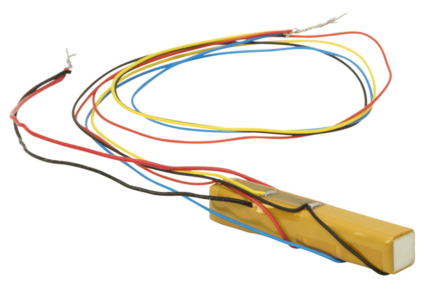
This work was based on a Thorlabs PK4FYC2 PEA (
Figure 1) which is a discrete stack actuator with four attached metal foil strain gauges in a full-bridge Wheatstone circuit (see specifications in
Table 1). The stack consists of multiple piezoelectric chips which are attached with epoxy and glass beads. The maximum displacement provided is 38.5
m at the maximum drive voltage whereas the hysteresis can induce an error of 15% according to the manufacturer.
Since the displacement measurement device is a strain gauge made of resistances configured as a Wheatstone bridge, certain issues had appeared at the moment of the measurement and it was concluded that the environment temperature had an impact on it. Cappa [
21] provided proof to this hypothesis since these type of gauges are affected due to the change in thermal expansion coefficient. For this reason, all the experiments were conducted on the same day and time.
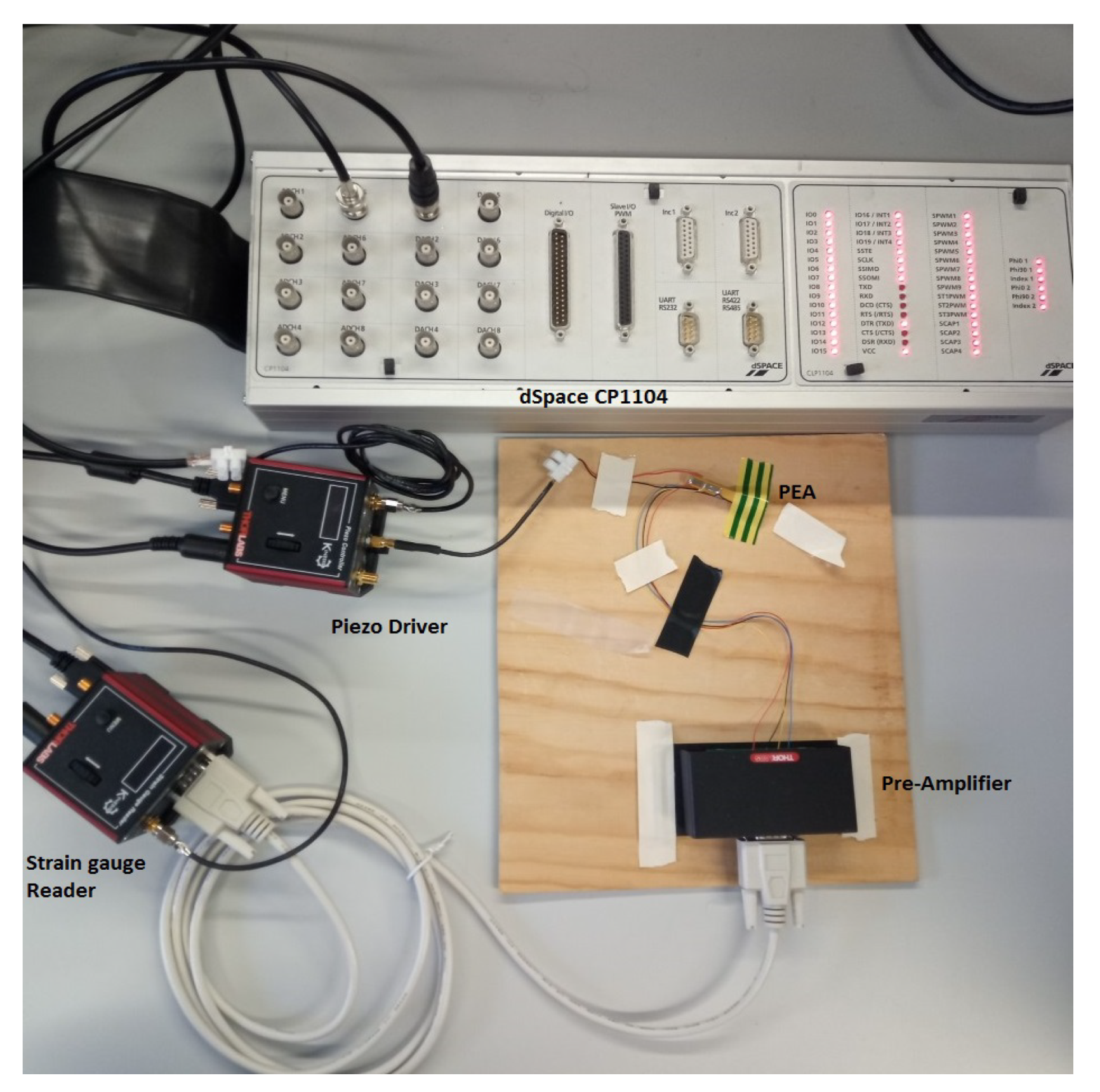
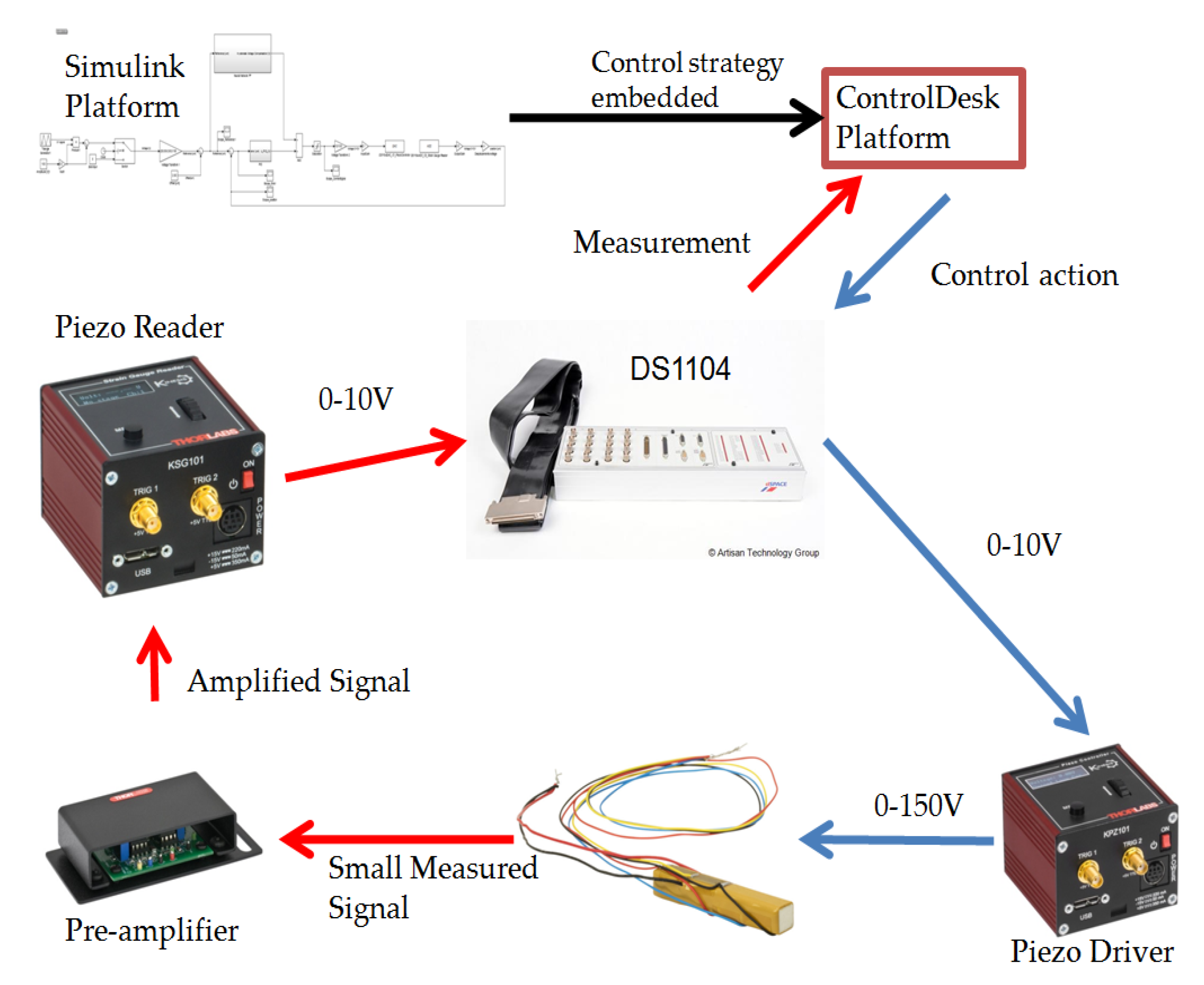
Figure 2 and
Figure 3 expose the control architecture which was designed in Simulink and embedded on ControlDesk platform within a dSpace controller board DSP1104 which granted 0–10 V range to driver cube. The hardware that provided the driving voltage was a PEA Controller Driver (KPZ101 by Thorlabs) which can supply up to the maximum PEA voltage and it can work in open as well as close loop, like in this research.
The measured displacement voltage that the strain gauge provides is between 0 and 2 V. As this is a minuscule signal, a pre-amplifier AMP002 by Thorlabs was linked with the strain gauge reader (KSG101 by Thorlabs) where the output is a voltage between 0–10 V. Finally, dSpace hardware reads the signal which was displayed in ControlDesk platform.
Pea Hysteresis Analysis
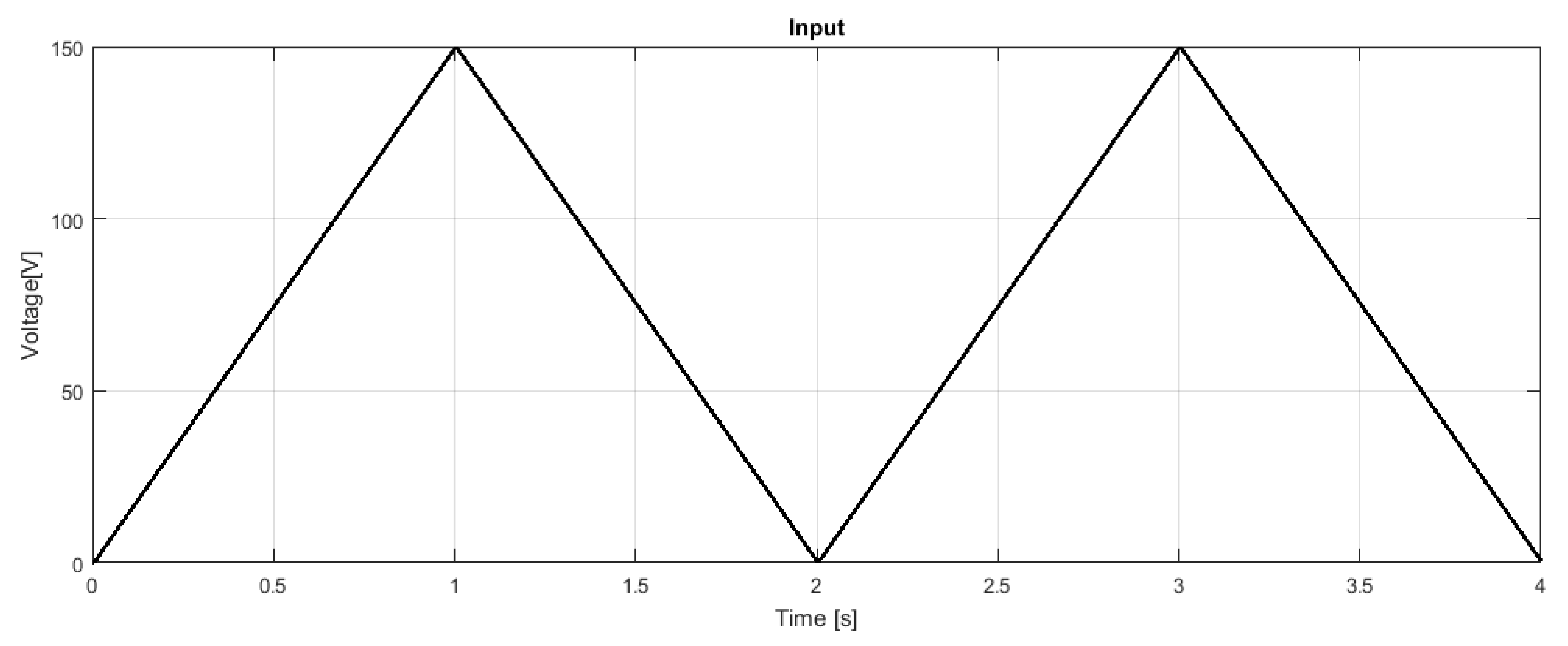
The main non-linearity analysed in this research was based on hysteresis that affected enough the performance of the PEA at guidance during the desired position. This investigation used a triangular wave (
Figure 4) since this function reflects vastly superior the hysteresis than others and also it can be considered as the sum of infinite harmonics and thus, the control tracking needs to be more robust and precise than with a softer signal like a sine wave. The sampling time was set at 1 kHz to drive the PEA since it was found to be optimal with the data acquisition and the hardware limitation.
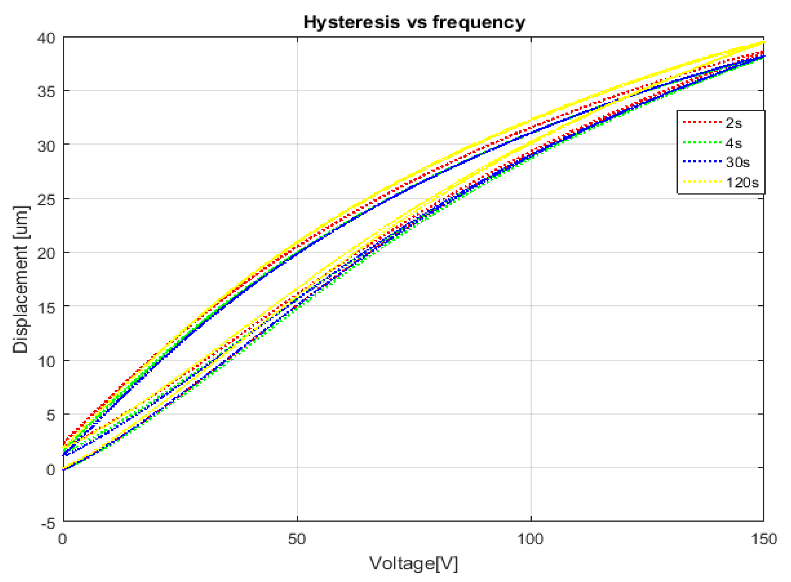
The period of the triangle wave was not chosen arbitrarily due to the following shallow analysis. PEA resonant frequency is 34 kHz, so the period needed to be far from the inverse of this value.
Figure 5 displays how the PEA performs at different periods for a triangular wave at maximum driving voltage. Hence, 2 s was chosen since covers an average of all the tested samples, although the highest difference can be seen at the maximum voltage.
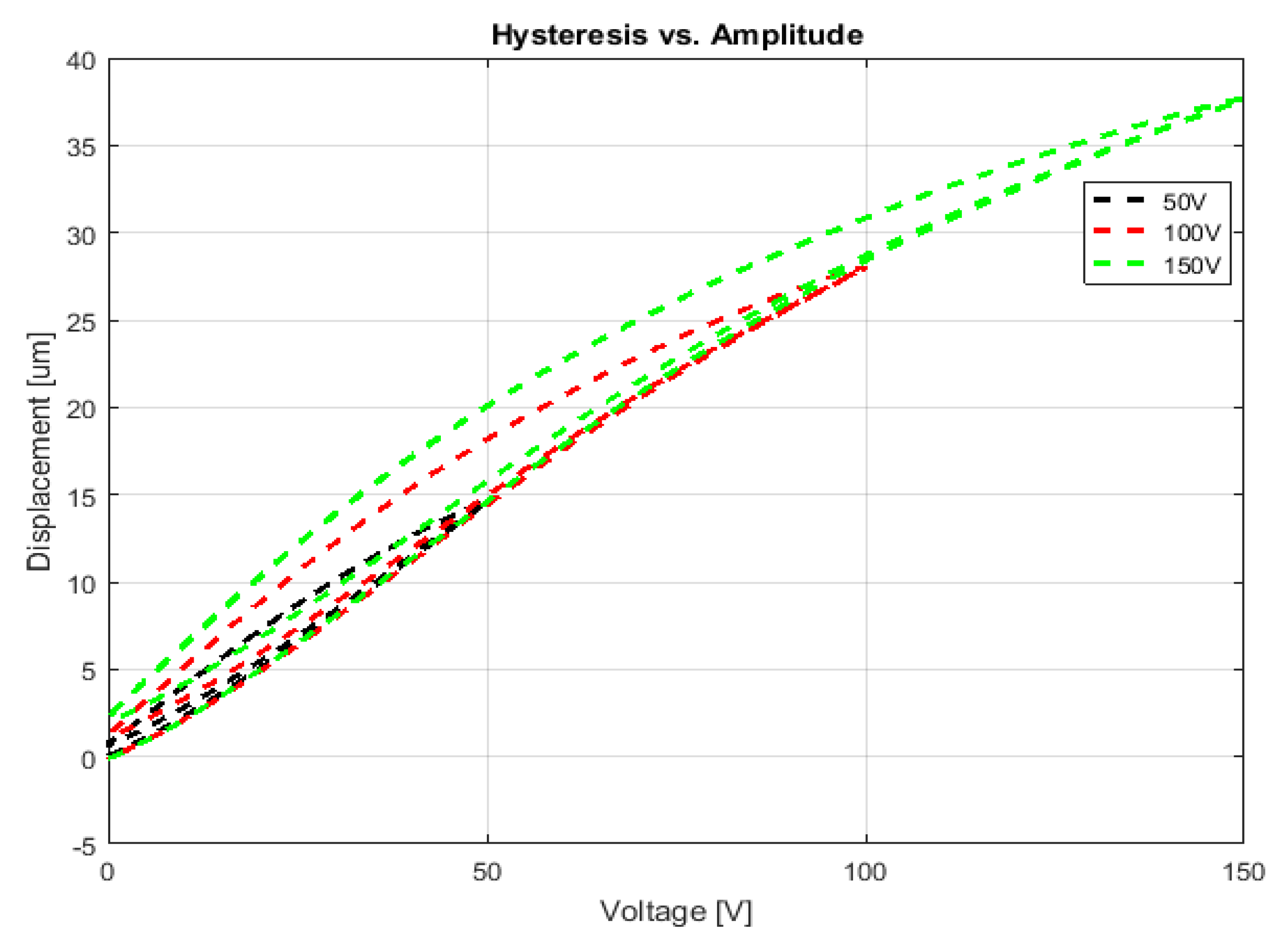
Regarding to the amplitude,
Figure 6 shows how the hysteresis behaves with different voltages. Although the non-linearity appears at lower voltages such as 50 V, it can be seen that at 150 V the hysteresis prevails more than with lower values. For this reason, the whole analysis realized during this research was done under the mentioned amplitude and the chosen input signal period.
3. Hysteresis Fitting with NN
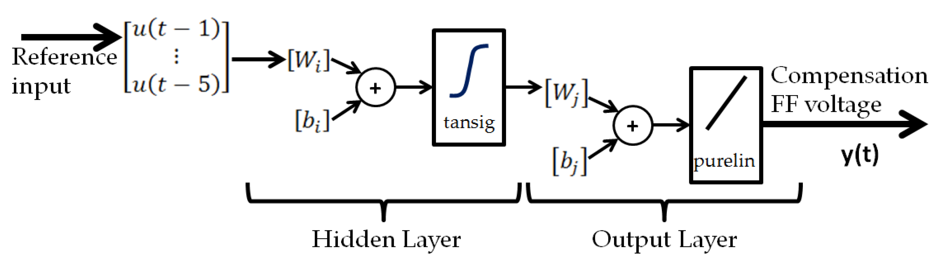
The PEA non-linearity hysteresis can be considered as a mapping problem since there can be two values for input, thus ANNs have many advantages such as self-learning and simplicity, which is suitable to learn one hysteresis curve. The ANN architecture used to fit the hysteresis loop was a Time Delay Neural Network (TDNN) which is a variance of a NARX but where the input weights have tap delays associated. Hence, the output prediction
y(t) depends on past values of the input and is combined with a non-linear function
f. In this case, the number of delays chosen was 5, due to the default configuration of Matlab Deep Learning Toolbox.
The complexity avoidance can result as the function
f is approximated to a combination of a hidden and an output layer where each has its weights and activation functions. Regarding the training information, a triangle wave with the previously mentioned features was used to obtain information for 10 s such as the displacement. In terms of the training algorithm, Matlab ANN toolbox suggests using as a first try, due to the fast back-propagation, the Levenberg–Marquardt (LM) which updates the weights and bias in terms of a back-propagation and optimization where the main metric is the mean squared error (MSE). Boussaada [
16] provided a deep analysis of different training algorithms where it was found that LM supplied efficient results. Since the FF compensation was expected in terms of voltage, an inverse model was needed; then, the input voltage used to obtained the hysteresis was the ANN target and the displacement as the input.
The
Figure 7 displays the architecture of the TDNN where the weights and bias are different of in each layer in terms of the subscripts
i and
j respectively. The hidden layer uses a Tansig activation function whereas the output operates with a Purelin, which according to [
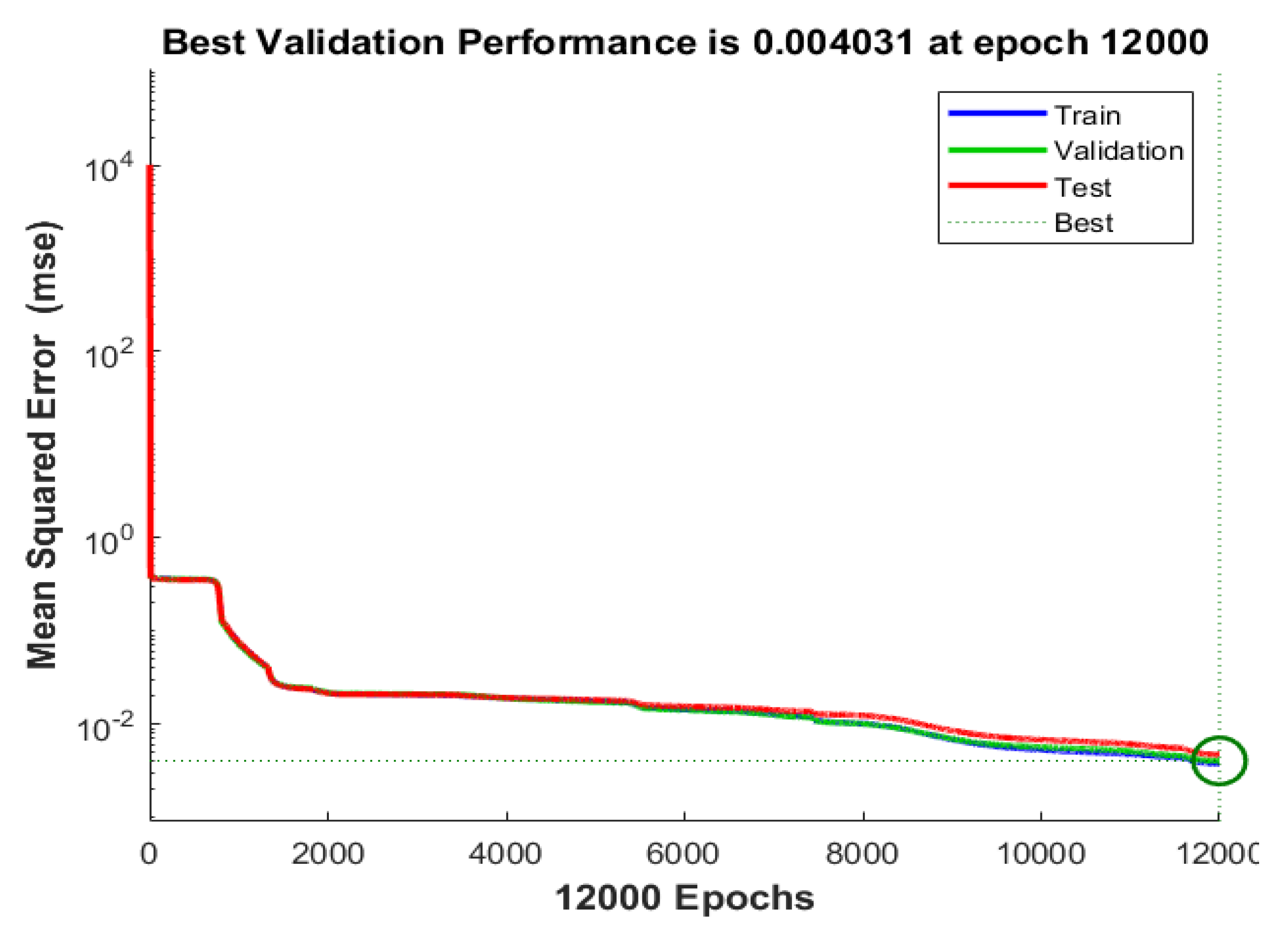
22], the configuration can approximate any function given the sufficient number of neurons. Based on a trial and error, the amounts of neurons were determined on a range from 5 to 30 and the optimal one was found to be 22 in which the MSE was 0.004031. The convergence development was found to be optimal since the following curves showed that model over-fitting was not an issue as
Figure 8 shows.
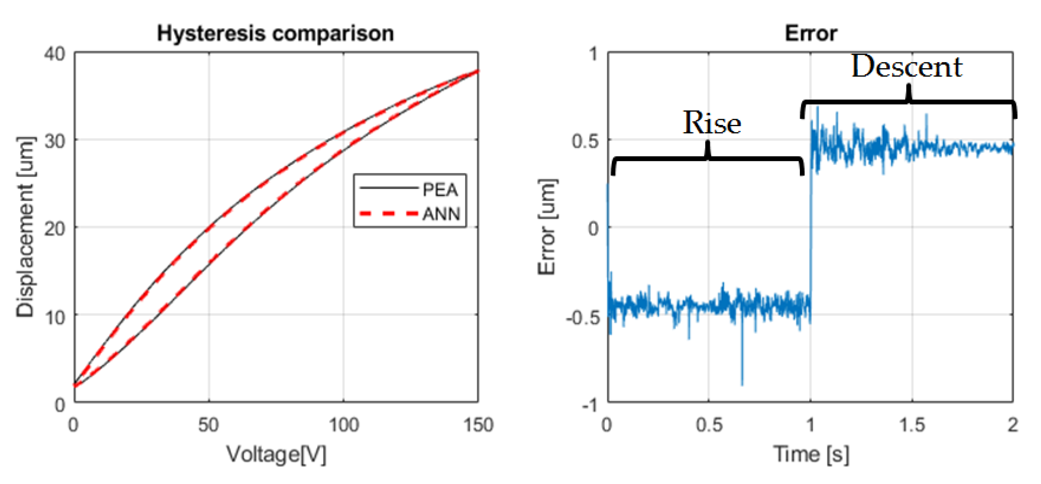
Figure 9 is a comparison with the piezoelectric hysteresis loop and the ANN fitting with the error on the right-hand side. Even though that the MSE was sufficiently small, the error in the comparison is around 0.5
m which is acceptable, but even more interestingly the ANN could manage the asymmetrical shape that belongs to the device. The error compensation was expected to be done by the feedback controllers which were implemented.
4. Control Structure
At the beginning of the experiments, simple and classical algorithms were tested where the following steps consisted of increment complexity so that the efficiency could be improved. As all solutions were based on real tests, the controllers were tuned in real-time to achieve the best performance. As previously mentioned, there were four structures which were evaluated:
PID without FF compensation
PID with Linear FF compensation
PID with ANN FF compensation
SNPID with ANN FF compensation
The comparison was done with the first three systems since the PID was considered as the same in each (invariable , and ). In every structure, it was considered that the hysteresis loop curve was not the first try since, as previously shown, the initial rise is completely different from the following ones. The best result of these three architectures was contrasted with the fourth one, which is an ANN FF compensation with SNPID since the performance was expected to be superior to others.
Figure 10 is an schematic Simulink block diagram which was equal for all the architectures except for the close-loop controller and FF compensation. The First block is the triangle reference in voltage which afterwards was transformed into displacement where the initial offset was concerned. The output of this arrangement was the displacement reference which needed to be followed and was the input to the FF compensation. The PEA input signal was saturated (the use of more than 150 V can reduce the life of the device) and transformed into 0–10 V for the dSpace board. The output of the hardware was then converted into 0–10 V and displacement. During the experiments, it was found that the relation between the output voltage and the measured position had a factor of 4.
The performance of each framework was compared using the integral of the absolute magnitude of the error (IAE) over time as a metric, which has the expression of Equation (
2). The use of the error magnitude in the integral results in a sensitive expression either for positive or negative values.
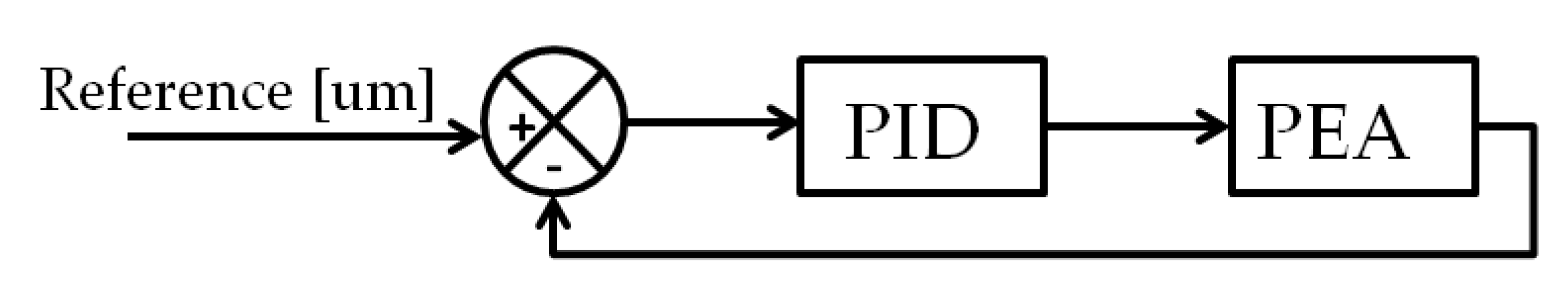
4.1. PID without FF Compensation
First, a simple and classic approach based on feedback structure was used with a PID controller (
Figure 11). Certainly, this might no be the most accurate aisle but was an acceptable starting point to undertake the following frameworks. The conventional PID Equation (
3) was embedded into the Simulink canvas for the experiment.
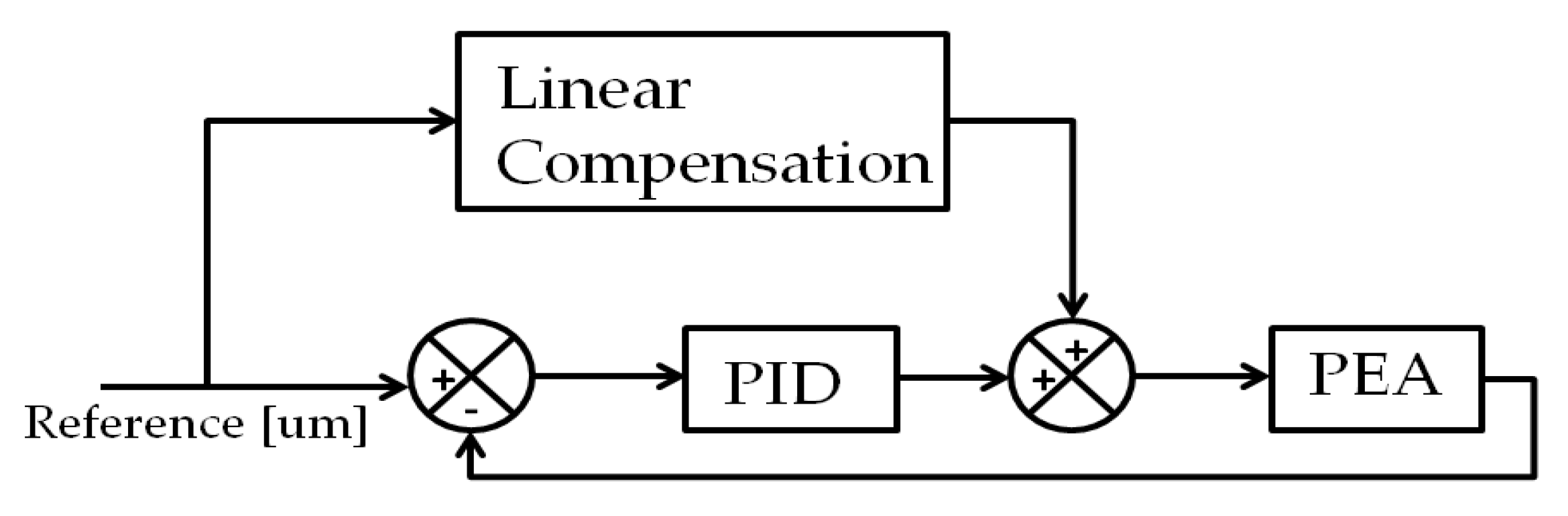
4.2. PID with Linear FF Compensation
The second approach proposed was a linear compensation with the previous PID (same constants) as
Figure 12 shows. Surely, in this case, the linear FF block is a supposition that considers that the PEA behaves linearly as well. Consequently, this was reflected as the
Figure 13 displays where the maximum and minimum displacement were used to generate a straight line that could resemble the linearity. In this circumstance, the feedback controller was expected to produce more compensation due to the hypothesis previously mentioned as the errors increased.
Since the hysteresis has a different shape during the first cycle in which the PEA starts at zero displacement and the following periods tend to a convergence where the initial displacement is not zero anymore due to the device properties and therefore, the curves are in a path to a common shape. During this research, a linear compensation was taken into account and hence, a straight line was interpolated between the initial offset and maximum value since the PEA was not expected to work only during the first cycle.
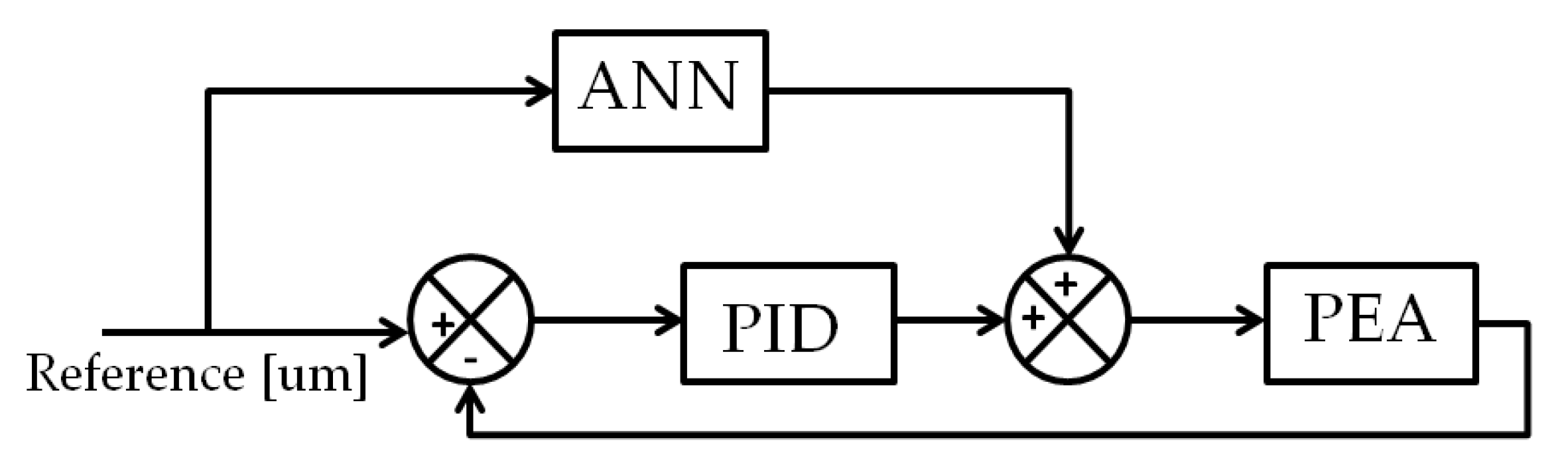
4.3. PID with ANN FF Compensation
A linear compensation might not be the best option since it can deliver enough error due to the high non-linearity during the whole cycle. Nevertheless, the FF can be non-linear using the mentioned ANN obtained (
Figure 14). The system explained in
Section 3 was used as an inverse PEA model which behaves with better precision than a straight line. Hence, it was expected that the guidance performance was going to increase compared to the architectures previously presented.
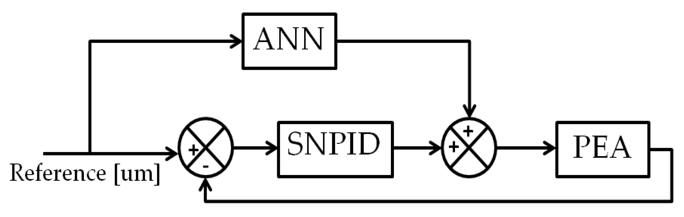
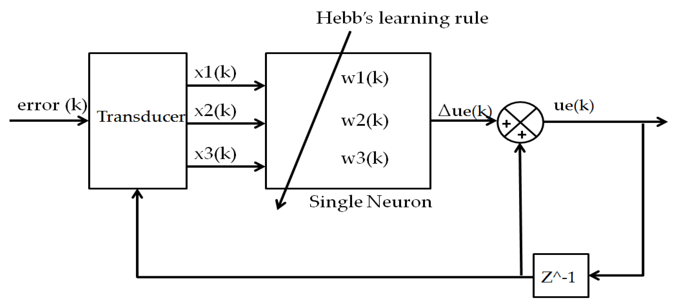
4.4. SNPID with ANN FF Compensation
Even though the performance could increase with the previous architecture, PID constants were still switched by trial and error but since the system has sufficient non-linearity, the constants might not be optimal in each moment. Therefore, an optimization path for the controller could increase the demeanour (
Figure 15). The avoidance of manual tuning was found to be possible with a self-adaptive PID. The error input to the controller was discomposed into three variables (
,
and
) in a similar way to a conventional PID but there will be three associated weights (
,
and
) which are adjusted by normalization and a learning rate. Therefore, the Hebb supervised learning rule is used to self-tune the weights and the whole controller behaves like a “single neuron”; this is a non-linear process unit which is helped by the mentioned rule to adapt for a control process.
The error that went through decomposition or also called “transducer”, complied with Equation (
4), which is an expression that is related to a conventional PID controller as well. The three new variables were fed into the single neuron with the learning where the algorithm corresponds with the Equations (6). Afterwards, the output of the SNPID is the
which is finally added with the delayed signal like in
Figure 16.
Based on [
16], the weight that is more important due to environment is mainly akin with
and
and then, a simplification of the previously presented equation can be achieved where the main control structure is related to a weight update with the following normalization for calculation cut down and final control law.
5. Experimental Practices and Results
The experiments were obtained from the hardware distribution that is displayed in
Figure 2, where the four architectures were tested. The presentation began from an elementary PID (no FF compensation); the following comparisons were merged to show up the performance improvement as the complexity increases. Finally, the last comparison was made with two most sophisticated ones since the guidance, error and control signal were more suitable to compare.
The PID gains were obtained from a trial and error in real-time during the first three experiments, where the values are shown in
Table 2. Furthermore,
and
were increased respectively to limits where the input voltage was not critical for the device. On the other hand, the SNPID constants such as K were switched in real-time as well on the same way whereas the learning rates
,
and
were assumed as less than 0.5 as the references suggested [
20], in this manner were set to 0.4. The constants of SNPID are summarized in the
Table 3.
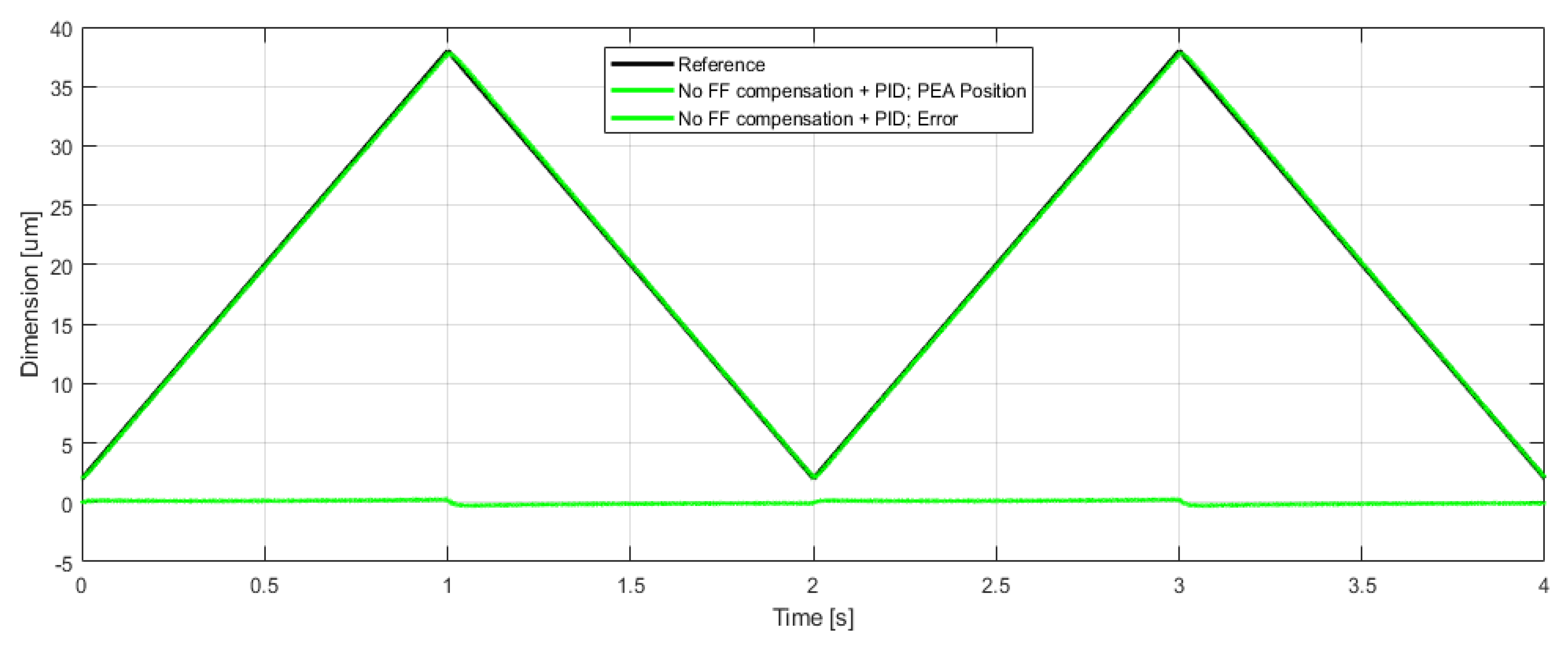
5.1. PID without FF Compensation Results
The first experiment was the close feedback loop with a PID as a controller.
Figure 17 displays the guidance embedded with the error where it can be seen that the peaks of the signal reduced the control performance since there was a sign change in the behaviour. In the following sections, this feature will be analysed in depth. The IAE had a value of 0.578 during the period that is shown and it will be compared with the following results.
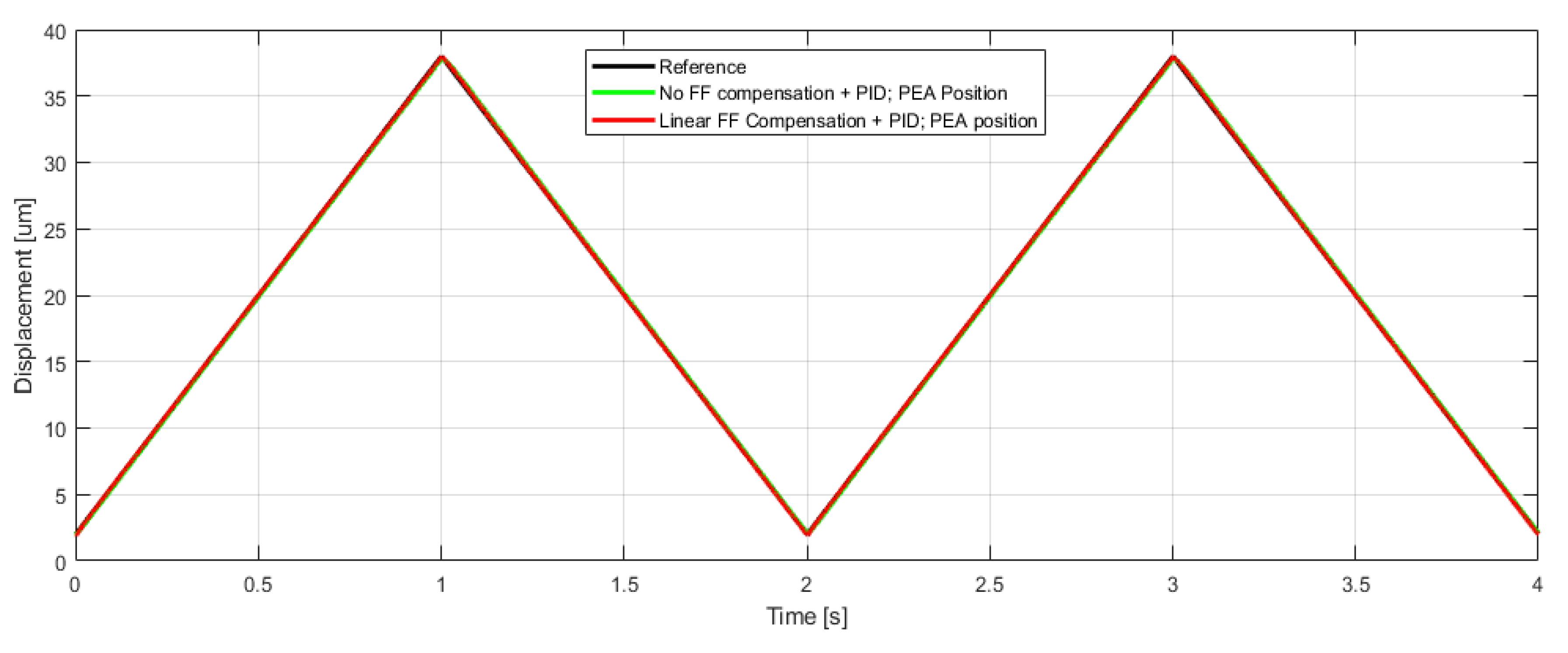
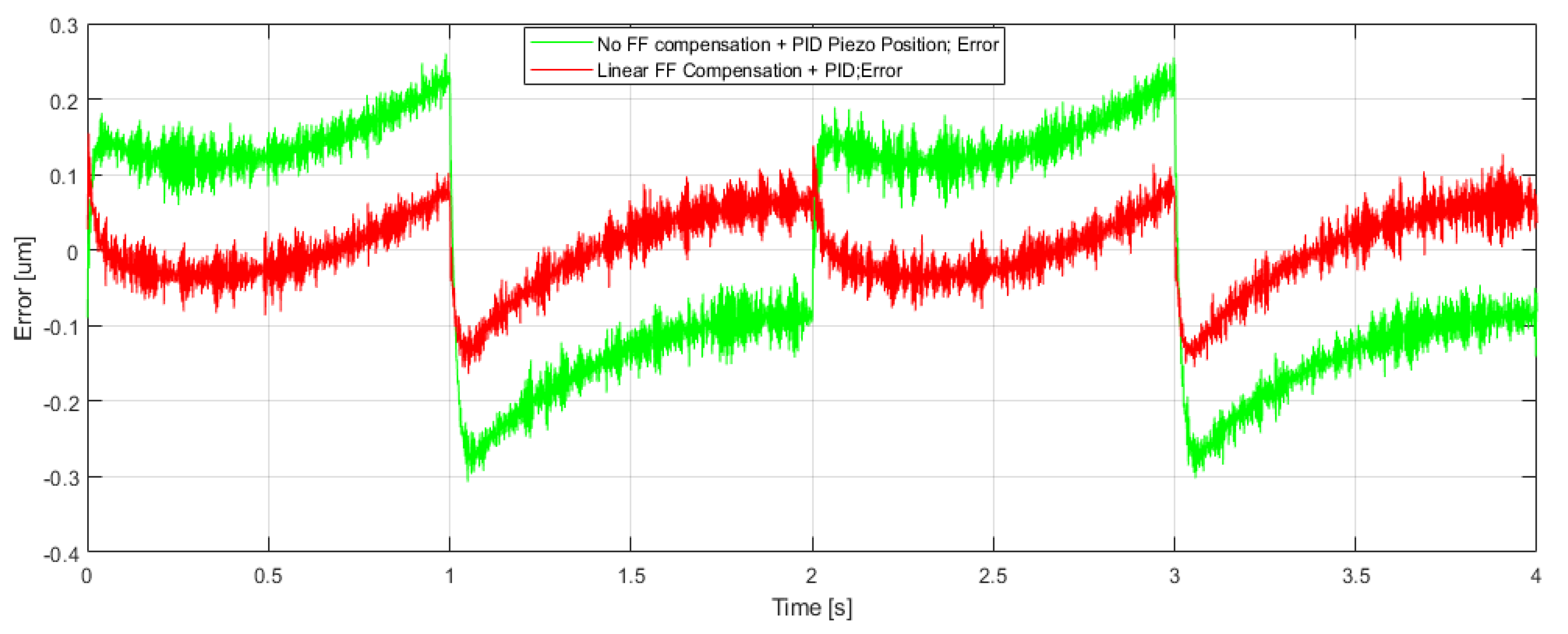
5.2. PID with Linear FF Compensation Results
The second try is a contrast with the previous showed result but now with a linear FF compensation. The new architecture increased the performance since the guidance and error were worthy reduced as it is shown in the
Figure 18 and
Figure 19 respectively, due to the FF addition. For this reason, the guidance efficiency had increased substantially although the values are still unreliable for a precision device. The IAE values had significantly decreased to 0.1659, which is 3.48 times less due to the improved framework.
5.3. PID with ANN FF Compensation Results
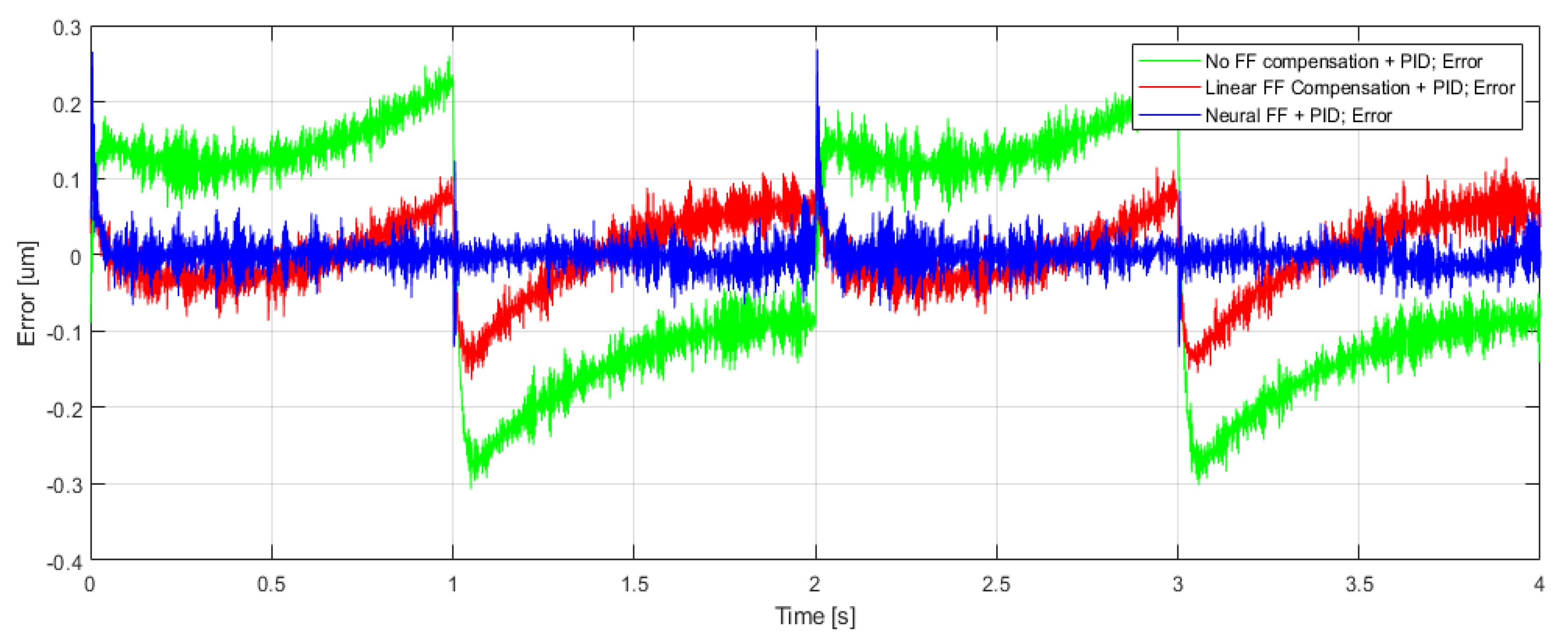
Certainly, the addition of a sophisticated FF compensation such as an ANN was expected to improve the performance and this was reflected in
Figure 20 and
Figure 21 where the tracking had improved adequately. The error is fairly reduced compared to the previously presented architectures and for this reason, it will be analysed in-depth during the following subsection with the most advance framework. As it was also expected, the IAE was reduced to 0.0683 with this approach and this results on a 2.42 times less than the previous framework.
5.4. SNPID with ANN FF Compensation Results
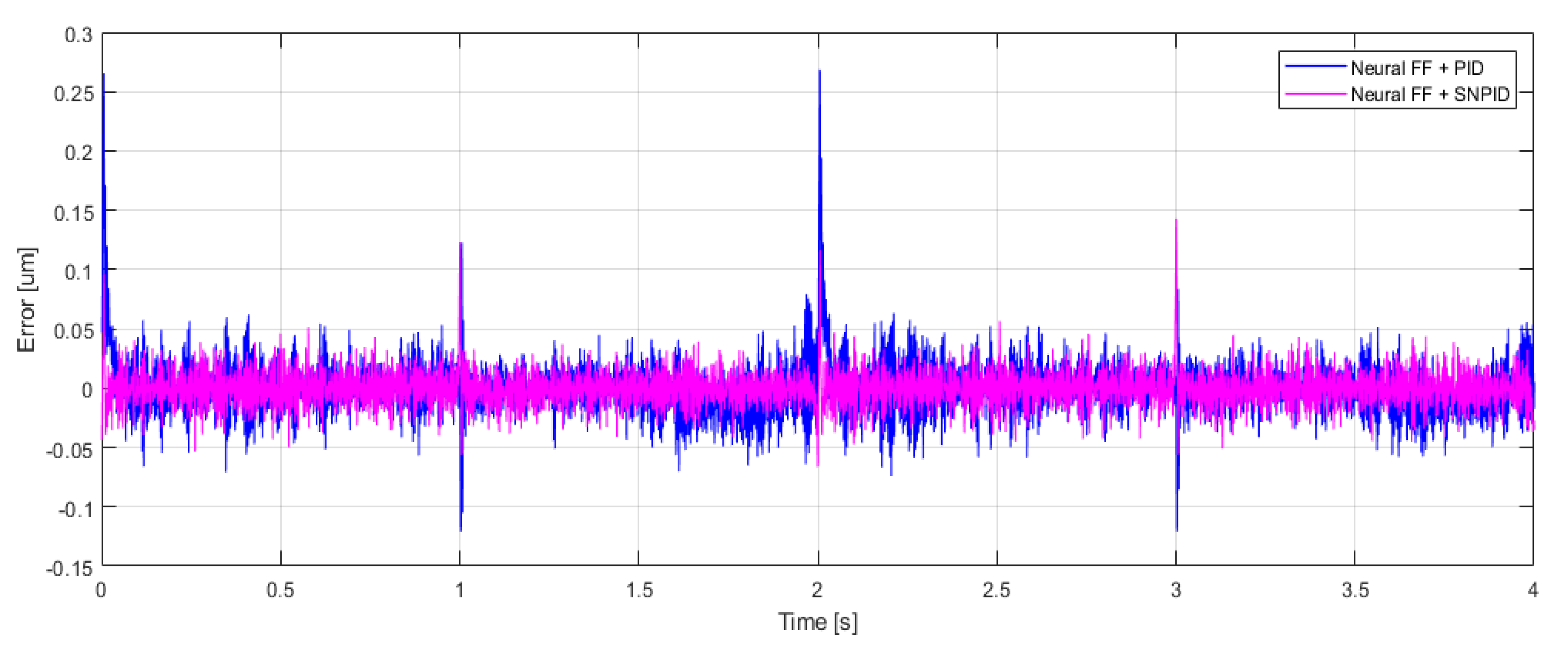
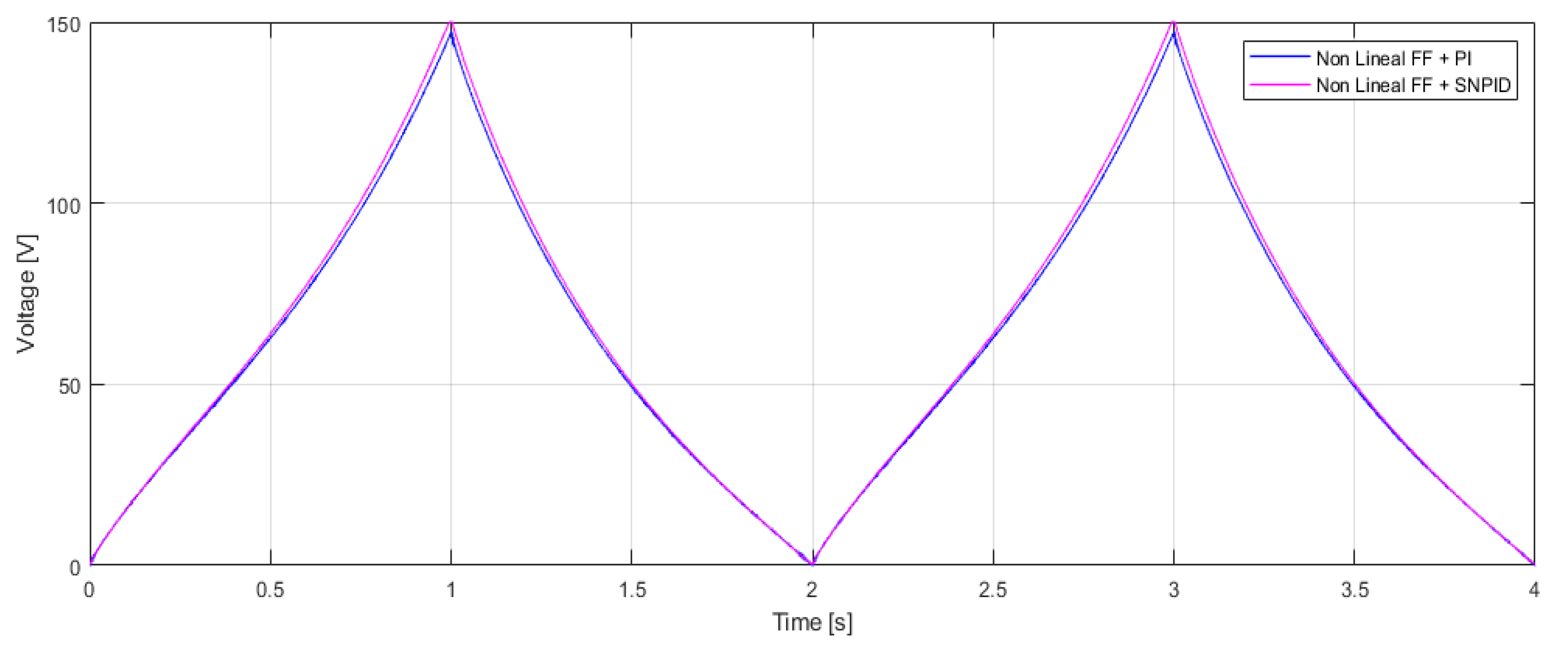
Finally, the last architecture tested was the SNPID. Since the results were close contrast regarding to guidance, the comparison was analysed with profundity especially in terms of error and control signal.
Figure 22 reveals the error progression along with two triangle reference as previously shown. The performance had undoubtedly increased since the mean error value tends to be very near to zero in both cases. However, the perception of the SNPID had increased essentially the efficiency around peaks (where the top values are in 1 and 3 s whereas the lower one is in 2 s). The FF with ANN compensation merged with the PID on feedback shows that after the lower peaks, the error increased its amplitude extensively and takes several fractions of a second to reduce it. Nevertheless, the framework with a SNPID corrects these effects with a small perception which resembles in a brief error increment which has less amplitude than the contrasted method; another advantage that can be appreciated is the fast error correction since the PID architecture had a slow demeanour to correct the error, the SNPID had the ability to avoid this situation.
On the other hand,
Figure 23 shows the control signal which is the sum of the feedback controller and the FF compensation. It can be seen that both signals are almost equal although and there were not any drastic changes or significant saturation which could reduce the lifespan of the actuator or make the system unstable.
As the analysis showed, this case had the best performance and this was reflected in the IAE. In this state, the value was 0.0499 which means that it has been reduced 1.36 times in contrast with the case from
Section 5.3. The
Table 4 is a comparison of all the IAE values that were exposed.
6. Discussion and Conclusions
This research has made a deep analysis of to compensate the hysteresis effect which started with elementary approaches until highly complex control algorithms in the feedback loop as well as in the FF which all of them, took place under experimental tests with real devices. Furthermore, the controllers were tuned under a rapid control prototyping type since most of the parameters were set in real-time to achieve the best performance for a genuine operation.
The analysis began with the device inspection in terms of frequency and different amplitudes where parameters were chosen to persist with the control design and especially, the ANN design. The FF neural compensation was first contrasted with real data in terms of the hysteresis. The result was acceptable since the interpolation had a small error which could be sufficient for the following compensation. The crucial improvement was the fitting along with the asymmetrical shape of the non-linearity since it was found in the references that this is a problematic feature to model with analytical techniques.
The first control architecture used was a simple one with a PID on the feedback where the results were as expected due to the high non-linearity presence of the device. The errors obtained were not acceptable since the position guidance was the main achievement to be improved. The following contrast was against a linear-compensation and certainly, it was found that even an inaccurate compensation could improve the performance since the IAE had a value of which was 3.48 times less than the first basic control architecture. Although the performance was improved, the value was still not sufficient because the linear interpolation was between two points of the hysteresis curve and this might not be the best solution, due to the asymmetric effect explained.
The last two approaches, which are the most complex ones, provided better outcomes than the previous ones. The addition of an ANN compensation surely was expected to provide better results since the fitting efficiency was higher due to the flexibility of the ANNs. As a result, the IAE decreases reasonably in comparison with the linear compensation and it resembled on the performance as it was showed (2.42 times less than the previous). Since this approach was found to be the best one until that point it was chosen for a final comparison with a SNPID which was already known for its high performance. The FF compensation with SNPID improved the process were the conventional PID had a weak response like after a peak. It was found that the SNPID neglects and corrects the errors during these violent slope changes. The IAE for the last framework result in dramatic decrease since the value was 1.36 times less than the third approach; for this reason, this method is considered to be the best of the ones that were tested.
Since the last two methods were found to have a satisfactory response, the control signal was studied. It was found that the control signals for both schemes were acceptable since there were no significant or fast action which can compromise the hardware due to input signal generated. For this reason, it is expected that both approaches can have a valuable (and probably much better) performance for a smoother curve like a sine wave since a triangular was chosen for its high complexity representation and requirement.
Future studies scheduled can be related to many options since these ideas are still widely open to different frameworks. The implementation of diverse learning rules for the SNPID like Delta Learning rate rule, Oja’s rule, etc. are an option since the changes are mostly in the controller expressions. Regarding to the FF, the combinations can be less restricted since the ANNs are probably more flexible and efficient tools than classic analytical ones.
Author Contributions
Conceptualization, O.B., J.V. and C.N.; methodology, O.B., I.C. and C.N.; software, C.N.; validation, C.N; formal analysis, O.B. and C.N.; investigation, O.B. and C.N.; resources, C.N.; writing—original draft preparation, C.N.; writing—review and editing, O.B. and C.N.; supervision, O.B. and I.C.; project administration, O.B. and J.V. All authors have read and agreed to the published version of the manuscript.
Funding
This research was funded by Basque Government and UPV/EHU projects.
Acknowledgments
The authors wish to express their gratitude to the Basque Government through the project SMAR3NAK (ELKARTEK KK-2019/00051), to the Diputación Foral de Álava (DFA) through the project CONAVAUTIN 2 and to the UPV/EHU for supporting this work.
Conflicts of Interest
The authors declare no conflict of interest.
References
- Peng, J.; Chen, J. A Survey of Modeling and Control of Piezoelectric Actuators. Mod. Mech. Eng. 2013, 3, 1–20. [Google Scholar] [CrossRef]
- Ozaki, T.; Ohta, N. Power-Efficient Driver Circuit for Piezo Electric Actuator with Passive Charge Recovery. Energies 2020, 13, 2866. [Google Scholar] [CrossRef]
- Bertotti, G.; Mayergoyz, I.; Damjanoivc, D. Hysteresis in Piezoelectric and Ferroelectric Materials. In The Science of Hysteresis; Elsevier: Oxford, UK, 2006; Volume 3, pp. 338–448. [Google Scholar]
- Frederik, F.; Minorowicz, N. Open loop control of piezoelectric tube transducer. Mech. Technol. Mater. 2018, 38, 23–28. [Google Scholar]
- Ang, W.; Garmon, G.A.; Khosla, P.; Riviere, C.N. Modelling rate-dependent hysteresis in piezoelectric actuators. IEEE Int. Conf. Intell. Robot. Syst. 2003, 2, 1975–1980. [Google Scholar]
- Kuhnen, K.; Janocha, H. Adaptive inverse control of piezoelectric actuators with hysteresis operators. In Proceedings of the European Control Conference, Karlsruhe, Germany, 31 August–3 September 1999; pp. 791–796. [Google Scholar]
- Kuhnen, K. Modeling, Identification and Compensation of Complex Hysteric and log(t) Type Creep Non-linearities. Control Intell. Syst. 2005, 33, 134–147. [Google Scholar]
- Rakotondrabe, M. Bouc-Wen Modeling and Inverse Multiplicative Structure to Compensate Hysteresis Nonlinearity in Piezoelectric Actuators. IEEE Trans. Autom. Sci. Eng. 2011, 8, 428–431. [Google Scholar] [CrossRef]
- Wang, D.H. Linearization of Stack Piezoelectric Ceramic Actuators Based on Bouc-Wen Model. J. Intell. Mater. Syst. Struct. 2011, 22, 401–413. [Google Scholar] [CrossRef]
- Chouza, A.; Barambones, O.; Calvo, I.; Velasco, J. Sliding Mode-Based Robust Control for Piezoelectric Actuators with Inverse Dynamics Estimation. Energies 2019, 12, 943. [Google Scholar] [CrossRef]
- Tan, X.; Iyer, R.; Krishnaprasad, P.S. Control of hysteresis: Theory and experimental results. Proc. SPIE 2001, 4326, 101–112. [Google Scholar]
- Song, J.; Kiureghian, A.D. Generalized Bouc-Wen Model for Highly Asymmetric Hysteresis. J. Eng. Mech. 2006, 132, 610–618. [Google Scholar] [CrossRef]
- Araújo, R.; Oliveira, A.; Meira, S. A morphological neural network for binary classification problems. Eng. Appl. Artif. Intell. 2017, 65, 12–28. [Google Scholar] [CrossRef]
- Gong, T.; Fan, T.; Guo, J.; Cai, Z. GPU-Based parallel optimization and embedded system of immune convolutional neural network. Int. Workshop Artif. Inmune Syst. 2015, 62, 384–395. [Google Scholar] [CrossRef]
- Sánchez, D.; Melin, P.; Castillo, O. Optimization of modular granular neural networks using a firefly algorithm for human recognition. Eng. Appl. Artif. Intell. 2017, 64, 172–186. [Google Scholar] [CrossRef]
- Boussaada, Z.; Curea, O.; Remaci, A.; Camblong, H.; Mrabet Bellaaj, N. A Nonlinear Autoregressive Exogenous (NARX) Neural Network Model for the Prediction of the Daily Direct Solar. Energies 2018, 11, 620. [Google Scholar] [CrossRef]
- Alyukov, A.; Rozhdestvenskiy, Y.; Aliukov, S. Active Shock Absorber Control Based on Time-Delay Neural Network. Energies 2020, 13, 1091. [Google Scholar] [CrossRef]
- Xie, H.; Tang, H.; Liao, Y. Time Series Prediction Based on NARX Neural Networks: An Advanced Approach. In Proceedings of the Eighth Conference on Machine Learning and Cybernetics, Baoding, China, 12–15 July 2009; Volume 3, pp. 1275–1279. [Google Scholar]
- Liang, Y.; Xu, S.; Hong, K.; Wang, G.; Zeng, T. Neural network modeling and sigle-neuron proportional-integral-derivative control for hysteresis in piezoelectric actuators. Meas. Control 2019, 52, 1362–1370. [Google Scholar] [CrossRef]
- Qin, Y.; Duan, H. Single-Neuron Adaptive Hysteresis Compensation of Piezoelectric Actuator Based on Hebb Learning Rules. Micromachines 2020, 11, 84. [Google Scholar] [CrossRef] [PubMed]
- Cappa, P.; De Rita, G.; McConnell, K.G.; Zachary, L.W. Using Strain Gauges to Measure Both Strain and Temperature. Exp. Mech. 1992, 32, 230–233. [Google Scholar] [CrossRef]
- Bai, M.; Zhao, X.; Hou, Z.G. Application of Neural Network to the Alignment of Strapdown Inertial Navigation System. Int. Conf. Intell. Comput. 2007, 4681, 889–896. [Google Scholar]
Figure 1.
Piezoelectric device with the Wheatstone bridge integrated for displacement measurement.
Figure 1.
Piezoelectric device with the Wheatstone bridge integrated for displacement measurement.
Figure 2.
Experimental setup with the involved hardware.
Figure 2.
Experimental setup with the involved hardware.
Figure 3.
Flow diagram of the closed loop working environment.
Figure 3.
Flow diagram of the closed loop working environment.
Figure 4.
Input voltage wave used for analysis.
Figure 4.
Input voltage wave used for analysis.
Figure 5.
Experimental hysteresis curves vs. different periods.
Figure 5.
Experimental hysteresis curves vs. different periods.
Figure 6.
Experimental hysteresis curves vs. different maximum voltages.
Figure 6.
Experimental hysteresis curves vs. different maximum voltages.
Figure 7.
Time Delay Neural Network (TDNN) architecture in terms of delay inputs.
Figure 7.
Time Delay Neural Network (TDNN) architecture in terms of delay inputs.
Figure 8.
Mean squared error (MSE) vs. trained epochs.
Figure 8.
Mean squared error (MSE) vs. trained epochs.
Figure 9.
Hysteresis fitting with Artificial Neural Network (ANN) and the associated error.
Figure 9.
Hysteresis fitting with Artificial Neural Network (ANN) and the associated error.
Figure 10.
Simulink block diagram used for experiments with feed-forward (FF).
Figure 10.
Simulink block diagram used for experiments with feed-forward (FF).
Figure 11.
Simple proportional-integral-derivative (PID) on feedback.
Figure 11.
Simple proportional-integral-derivative (PID) on feedback.
Figure 12.
PID on feedback and linear compensation on FF.
Figure 12.
PID on feedback and linear compensation on FF.
Figure 13.
Linear interpolation.
Figure 13.
Linear interpolation.
Figure 14.
PID on feedback and ANN compensation on FF.
Figure 14.
PID on feedback and ANN compensation on FF.
Figure 15.
SNPID on feedback and linear compensation on FF.
Figure 15.
SNPID on feedback and linear compensation on FF.
Figure 16.
Single neuron PID (SNPID).
Figure 16.
Single neuron PID (SNPID).
Figure 17.
Comparison of guidance and error with a PID as a controller in the close loop.
Figure 17.
Comparison of guidance and error with a PID as a controller in the close loop.
Figure 18.
Comparison of guidance with a PID as a controller in the close loop contrasted with a linear FF compensation.
Figure 18.
Comparison of guidance with a PID as a controller in the close loop contrasted with a linear FF compensation.
Figure 19.
Comparison of error with a PID as a controller in the close loop contrasted with a linear FF compensation.
Figure 19.
Comparison of error with a PID as a controller in the close loop contrasted with a linear FF compensation.
Figure 20.
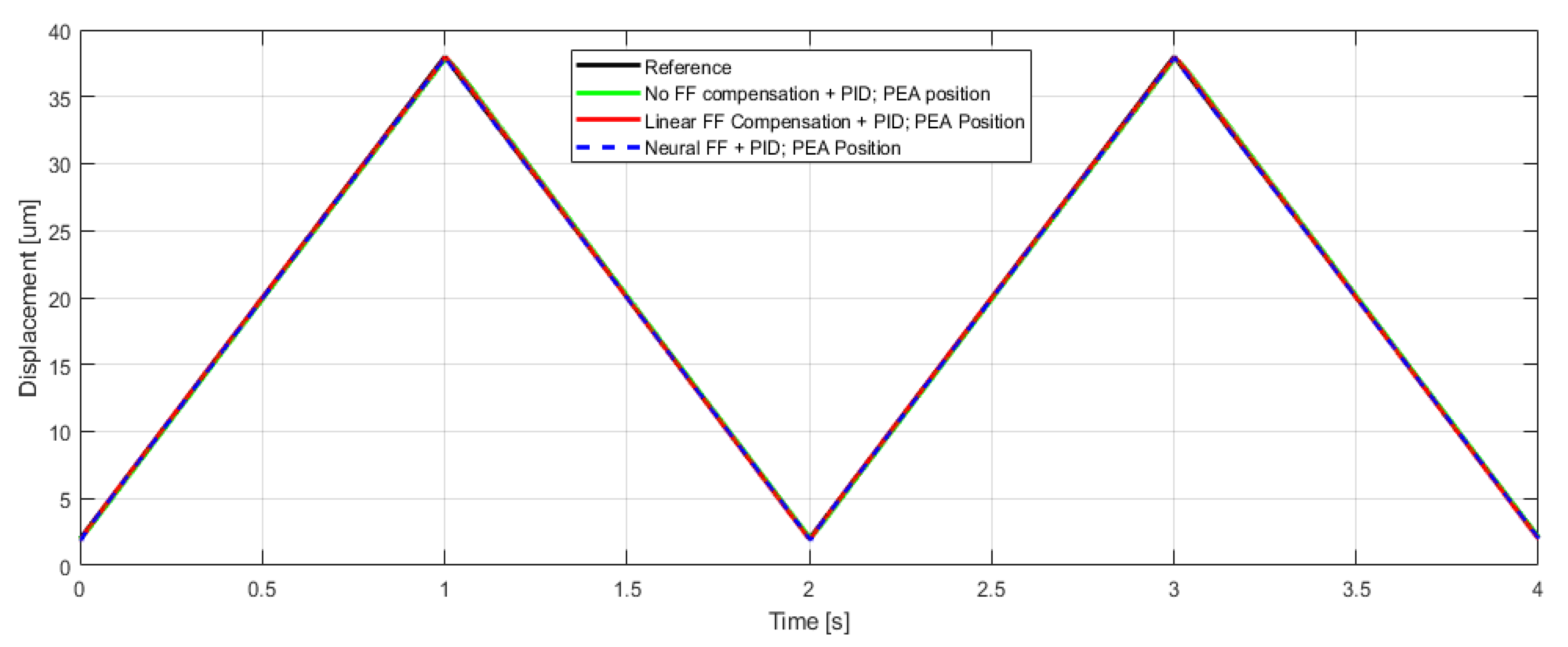
Comparison of guidance with a PID as a controller in the close loop contrasted with linear and ANN FF compensation.
Figure 20.
Comparison of guidance with a PID as a controller in the close loop contrasted with linear and ANN FF compensation.
Figure 21.
Comparison of error with a PID as a controller in the close loop contrasted with linear and ANN FF compensation.
Figure 21.
Comparison of error with a PID as a controller in the close loop contrasted with linear and ANN FF compensation.
Figure 22.
Error comparison with a Neural FF compensation with a conventional PID and a SNPID.
Figure 22.
Error comparison with a Neural FF compensation with a conventional PID and a SNPID.
Figure 23.
Control signal of a Neural FF compensation with a conventional PID and a SNPID.
Figure 23.
Control signal of a Neural FF compensation with a conventional PID and a SNPID.
Table 1.
Thorlabs PK4FYC2 specifications.
Table 1.
Thorlabs PK4FYC2 specifications.
| Properties | Values | Units |
|---|
| Physical Dimensions | 7.3 × 7.3 × 36 | mm |
| Nominal displacement | 38.5 | m |
| Max Force | 1000 | N |
| Drive Voltage Range | 0–150 | V |
Table 2.
PID parameters value.
Table 2.
PID parameters value.
| Constant | Value |
|---|
| 10.6 |
| 1000 |
| 0 |
Table 3.
SNPID constants value.
Table 3.
SNPID constants value.
| Constant | Value |
|---|
| K | 8.5 |
| 0.4 |
| 0.4 |
| 0.4 |
Table 4.
Integrals of the absolute error (IAEs) comparison.
Table 4.
Integrals of the absolute error (IAEs) comparison.
| Controller | IAE |
|---|
| PID | 0.578 |
| PID + Linear FF | 0.1659 |
| PID + Neural FF | 0.0683 |
| SNPID + Neural FF | 0.0499 |
© 2020 by the authors. Licensee MDPI, Basel, Switzerland. This article is an open access article distributed under the terms and conditions of the Creative Commons Attribution (CC BY) license (http://creativecommons.org/licenses/by/4.0/).


