1. Introduction
The increased electrification of the transport sector increases the potential use of renewable energy in electricity grids. This introduces challenges regarding the reliability of the power supply because on the one hand, renewable energy sources are mainly intermittent and therefore less predictable, and on the other hand they differ from “traditional” power generators in terms of circuit topology and effects on the grid. Top-down, centralized power flows change to more decentralized power generation, enabling the development of microgrids [
1,
2]. Power electronics (converter-based devices) are efficient for the conversion of power from DC to AC and vice-versa and are more often used for higher powers. This introduces several known and unknown effects in the grid at a large scale. One of the effects is the so-called “supraharmonic” disturbances (between 2 and 150 kHz), of which self-commutated converters are a significant source [
3,
4]. They can cause degradation of components due to excessive heating and malfunction or interference with other devices [
5] and even the damaging of equipment [
6]. Traditionally, supraharmonic (SH) disturbances were of less interest, but the expected increase in electric vehicles and fast chargers in both terms of quantity and charge power [
7] also increases supraharmonic emission and the corresponding consequences [
8,
9]. This development introduces the need for additional research and models of supraharmonic emissions from these devices in electricity grids and the possible impact they can have on the grid and all connected equipment. Past research has developed harmonic [
10,
11] and time-domain [
12] models for electric vehicle chargers as well as for low frequency (50 Hz–2 kHz) propagation [
13], but it is unknown whether they are also applicable for the supraharmonic range and when considering electric vehicles. Furthermore, supraharmonic propagation towards the grid possibly depends on the number of devices connected, as previously described for an installation with LED lights [
14]. The emission towards the grid is highly dependent on the number of devices connected and the impedances of individual devices and the grid. It is of interest to research how electric vehicles act as emission sources and interact in different grid configurations (including the impedances and background emission levels).
The goal of this research is to provide insight into the propagation and possible interaction of supraharmonics from electric vehicle chargers. This information is needed to create models of electric vehicle (EV) chargers in the supraharmonic frequency range, as well as for modeling the propagation of these currents in a possible future grid. This will lead to a better understanding of the impact the supraharmonics from electric vehicles can have and how an installation or the grid transfers these distortions. The analysis of supraharmonic interaction is valuable information for the development of models for the EV charger itself and to create awareness about these possible additional effects.
The main contributions of this research are therefore as follows:
Insight into the emission and propagation of supraharmonics of individual and combinations of electric vehicles in a small, low-voltage grid;
The influence of the grid impedance on the supraharmonic emission of electric vehicles, covering the public supply and microgrid operation (supplied by a storage inverter);
An analysis of possible interactions between electric vehicles due to supraharmonics.
This paper is set up as follows. In
Section 2, theoretical background on supraharmonics and the different sources and effects on equipment is given. Then, the experimental setup for measuring the supraharmonic emission of individual vehicles in different grid conditions is described (
Section 3). Then the results of emission and propagation measurements are studied, the different factors influencing them are analyzed, and the results are discussed (
Section 4). During the measurements, supraharmonic interaction between the electric vehicles is observed. This is further analyzed, and their occurrence is explained by simulations and theory in
Section 5. Finally,
Section 6 summarizes the results and gives the most important conclusions, and in
Section 7, recommendations for further research are given.
2. Background on Supraharmonics
Supraharmonics have been known about for a long time, but the amount of research on this topic has remained very limited. The definition of “supraharmonics” is proposed to describe waveform distortion in the frequency range of 2–150 kHz and is widely adopted [
15]. The lower limit (2 kHz) is taken to be equal to the upper limit of the traditional PQ-standards, covering up to the 40th harmonic. They were traditionally assessed for line-commutated converters, but self-commutated converters have emissions not related to the fundamental frequency and can easily reach much higher frequencies. The upper limit is chosen as the lower limit of the electromagnetic compatibility (EMC) standardization framework (150 kHz). Recently, research on supraharmonics has started growing and several standardization committees are working on describing emission and immunity limits as well as testing methods for disturbances in this frequency range [
16]. There are different reasons for studying emissions in the supraharmonic range. First, there is an increase in equipment emitting supraharmonic disturbances used by consumers, and secondly, power-line communication (PLC) makes use of the same frequency range [
17]. For example, smart meters, which are nowadays present in the majority of households in Europe, often use PLC over the low-voltage (LV) grid. Depending on the grid impedance, background emissions originating from other devices can influence the communication reliability [
18].
On the other side, the immunity of end-user equipment to supraharmonic disturbances has already been studied to some extent [
19]. Most electronic equipment uses EMC filters with capacitors to remove high-frequency noise from the input. However, capacitors absorb the high-frequency components as their impedance is inversely proportional to frequency according to
with
C being the capacitance and with the frequency
f in Hz. This can lead to extensive heating and decreased lifetime (up to 40%) of those components, resulting in degradation of the equipment itself [
20].
Furthermore, (linear) load-flow models that are useful for modeling the behavior of “classic” harmonics are not accurate enough to model the propagation of supraharmonics because they are often not directly linked to the fundamental frequency and their behavior in grids is difficult to predict. Interaction between the grid and EMC filters influences the amount of current absorbed by other devices and changes resonant frequencies [
21].
2.1. Primary and Secondary Emission
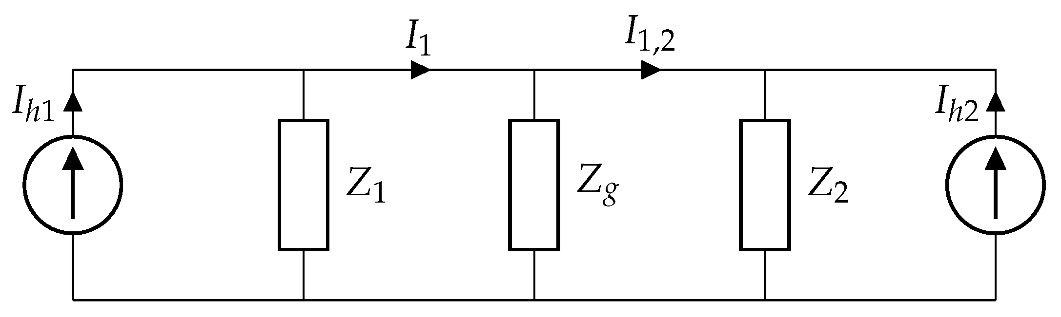
When studying harmonics, it is important to make a distinction between primary and secondary emission. This is needed in order to determine if part of the emission is originating from the device under test (DUT) or from another external source, thus defining responsibility. However, this is difficult because it is not always possible to isolate a single device to determine its primary emission [
16]. A simple and idealized model to understand primary and secondary emission is shown in
Figure 1. Here, device 1 is represented by a constant supraharmonic current source
and internal impedance
, which will absorb part of the emission. This will result in the primary emission from device 1 (
) as follows:
with
and
being the internal device impedances of device 1 and 2, respectively, and
being the grid impedance. This primary emission (
) is now partly flowing into the grid and a part through the impedance of device 2 as
where
is the secondary emission of device 2, originating from device 1. In the same way as described in (
2), the primary emission from device 2 can be determined. However, the total emission of device 2 will now be composed of the combination of its own primary emission
and the secondary emission from device 1 (
):
with
representing the primary and secondary emission of device 2. This effect will work in two ways; the total emission of device 1 will, therefore, also include part of the emission from device 2 that flows through the internal impedance
, resulting in a similar emission (
) for device 1. Background emission from the grid can be modeled as voltage source
, resulting in a current
through
and the device impedances. In practice, it is often not known how these impedances relate to each other, making it difficult to distinguish primary and secondary emission. Furthermore, it is difficult to determine the primary emission of a device when it is not connected to an ideal undisturbed grid. This research tries to distinguish between primary and secondary emission by using an environment in which turning devices on and off can be controlled.
2.2. Sources of Supraharmonics
There are different sources of supraharmonic emissions. In general, all devices with converter-based power electronics emit supraharmonics to a certain extent, as an artifact of the conversion from AC to DC or vice versa. In this research, only the effects on the power quality at the AC side are presented. Nevertheless, effects on the DC side can be present but fall outside the scope of this research. Next to the fact that power electronics are a prominent source of supraharmonics, they can also be key to mitigating distortion when the proper technology is used [
3].
When converting an alternating current to a direct current to, for example, charge a battery, different circuit typologies can be used. Most common in EV chargers and photo-voltaic (PV) inverters are bridge rectifiers with additional active or passive power-factor correction (PFC) circuits to keep the power factor (PF) around 1.
In [
22], the supraharmonic emissions of nine popular battery electric vehicle (BEV) types (representing 90% of the total share of BEV types in the Netherlands by the end of 2018) are measured. The results show that, except for one, all tested BEVs emit supraharmonic distortion to some extent and that most (6/9) use switching frequencies within the human hearing range (20 Hz to 20 kHz). This can lead to irritation and stress of the user.
An example of a measured current containing supraharmonic distortion from a single-phase BEV charging at 16 A is shown in
Figure 2. This superimposed 10 kHz component is visible with an average amplitude of 1 A (5% of the fundamental), but peak values go up to 2 A. The effect on the grid voltage is also shown, with, on average, 1 V at 10 kHz.
Other research also shows that electric vehicle chargers [
8] and bus chargers can be a source of supraharmonic distortions.
PLC uses a superimposed voltage on the fundamental with frequencies within the supraharmonic range (9 to 95 kHz). This is considered as intentional emission and, therefore, the limits for narrow-band signals according to EN-50160 apply. Supraharmonic current emissions from other devices, as artifacts of the AC/DC conversion, can also result in supraharmonic voltages. It has been observed that harmonic emissions moved from the classic harmonic range to the higher frequencies to avoid exceeding the existing limits for the frequency range below 2 kHz. From this point of view, the emissions from the converters should also be considered intentional [
4].
2.3. Supraharmonic Propagation
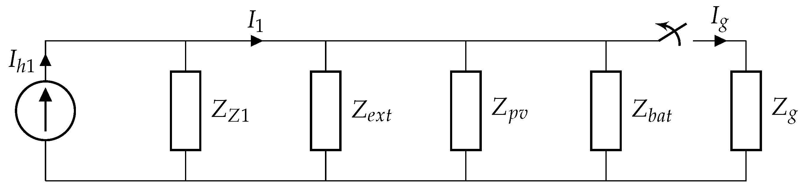
To study the propagation of supraharmonic currents originating from a single device, the model shown in
Figure 3 is used [
23]. Here, the constant supraharmonic current source
is used to represent harmonic current emission from the DUT. Impedance
represents the internal filter circuit of the device itself, absorbing part of the emission. Primary emission from device 1 is represented by
and obtained in a similar manner as in (
2). This harmonic load-flow model can be used for each individual device (1 to n) to model the propagation to other devices and the grid. For example the (supra)harmonic current originating from device 1 is flowing to the grid impedance
as follows:
with
being the impedances of other external devices,
and
being the PV- and battery-inverter impedance, respectively. This load flow can be made for each device, and by superposition, the total emission is determined. The grid impedance includes the impedance of the cable to the transformer and the transformer LV impedance [
23].
By switching between grid and microgrid mode, the grid impedance and background distortion in the voltage change. This can lead to a change in the emission of each connected device. Furthermore, it is assumed that the inverter impedances and are not constant for the different operation modes. This makes modeling difficult.
For low-voltage networks, the resistance is dominating, especially close to equipment. Hence, for low frequencies (<2 kHz) it can be assumed that is largely resistive. However, for higher frequencies the reactance of the cable will increase and can become dominant and the influence from impedances of neighboring equipment can play a role due to their capacitive nature.
Adding extra devices will create a different impedance seen by the device and will possibly affect supraharmonic emission. However, it is important to note that for each frequency, this model has different parameters, as device impedances (often capacitive due to filters) and grid impedances (often inductive due to cable and transformer characteristics) change with frequency. By superposition of all individual harmonic load-flow models per frequency, the total supraharmonic emission to the grid from the system can be determined. In this linear model, no interaction between devices or other effects are included.
2.4. Effects of Supraharmonics
From the skin effect, the current density in a good conductor will decrease exponentially from its value at the surface for increasing depth. The skin depth (
), or penetration depth, is dependent on frequency (
f) as follows:
with material permeability
and conductivity
[
24]. This means that higher frequencies will propagate more at the outer skin of a conductor, leading to a reduced effective usable section area and thus, a higher resistance. This will lead to additional heating of cables and other components connected to the grid. Furthermore, measurements on small distribution transformers showed the possibility of a transfer of supraharmonic currents to upstream grids as well, to a small extent [
25].
When studying supraharmonic disturbances, a distinction could be made between devices with communication (intentional emission, e.g., PLC) and without (emission as artifact). Besides the additional heating of components, effects like audible noises and the malfunction of equipment including PLC are described [
5]. Examples are whistling induction plates [
26], charging interruptions of EVs [
22], malfunction of coffee machines and failures of smart meters. For the latter, measurements show that some smart meters can be influenced by supraharmonic currents from PV panels by giving measurement errors up to –50%. This means the smart meter underestimates the amount of power delivered back to the grid, which is an adverse effect for the customer [
27]. Furthermore, LED drivers could be affected by supraharmonic disturbances, resulting in variations in the light intensity [
28].
3. Method
In this section, the measurement setup and process are described. To determine the primary supraharmonic emission of individual EVs and to see the effect of adding extra BEVs nearby on the secondary emission, different measurements are conducted. The goal of the measurements is to obtain insight into the propagation of the supraharmonic currents in the low-voltage installation. Because the charging current of BEVs is easily controlled and they are the main source of supraharmonics in this case, this is used as the main variable. All experiments are conducted twice—once for the lab connected to the public grid and once for the lab in microgrid operation (public grid disconnected). First, one BEV is measured and charged at different charge currents in order to obtain a complete overview of the supraharmonic emission of the BEV and to see whether it is dependent on the charge speed. Second, the same experiment is repeated for the second BEV, for the third, and for the fourth. Then, the combinations are tested. Again, the first BEV is measured during charging, but now, sequentially, the other BEVs are added to see the absorption of emission. In this way, a complete insight into the propagation of the supraharmonic currents from the individual BEVs is obtained. This is again repeated for all BEVs in the relevant possible combinations. Further in this section, the lab configuration, the measurement equipment, and the tested battery electric vehicles will be discussed.
3.1. The Lab: Microgrid and Public Grid Operation
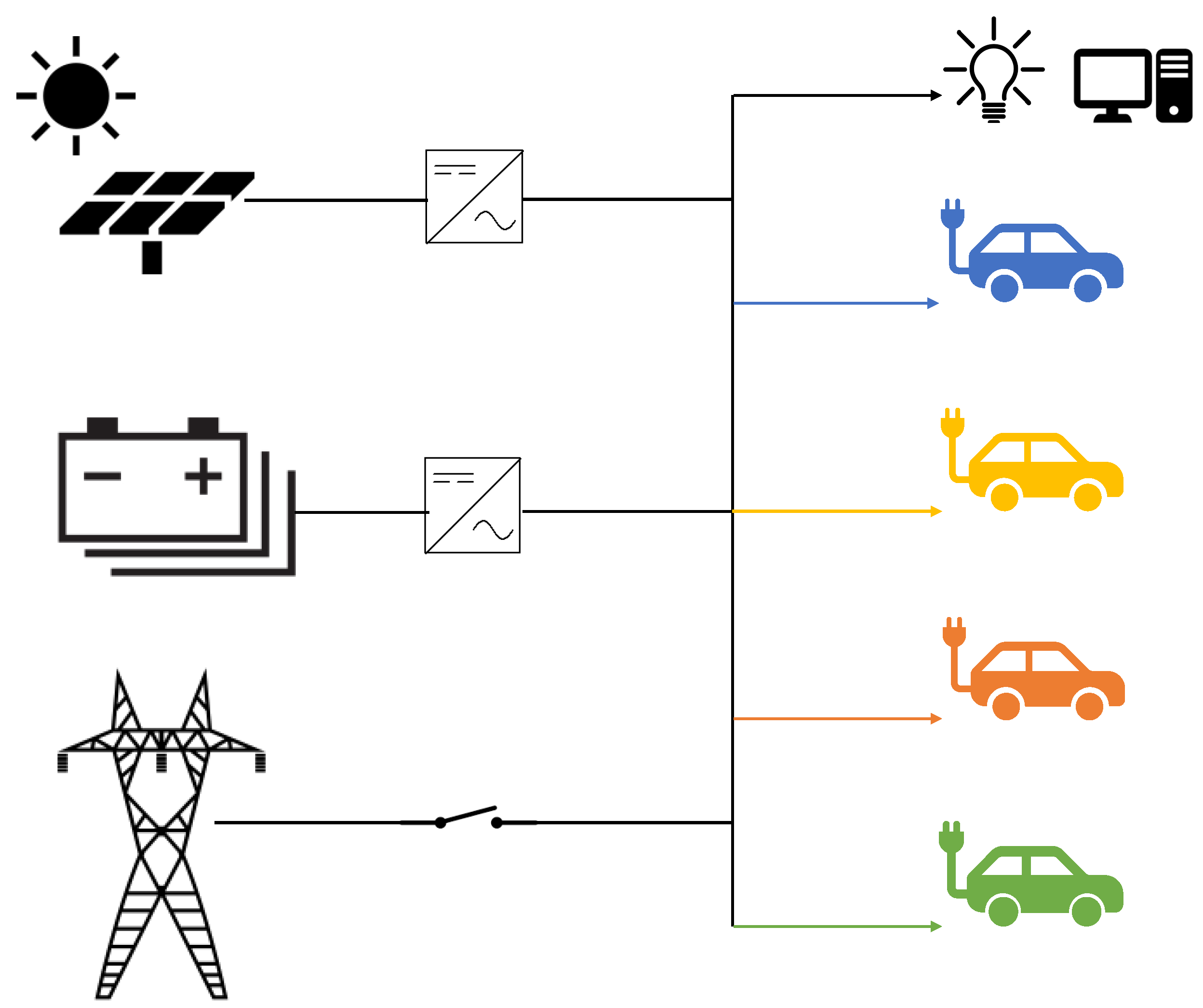
To test the interaction between converter-based devices with considerably high power for households, experiments were set up at the Smart Grid Interoperability Lab (SGIL) located in Petten, the Netherlands. This lab is part of the Joint Research Centre (JRC) of the European Commission. The environment is set up to represent a future household, with PV-panels, battery storage, and smart, energy-efficient appliances. This is a very unique configuration and enables experimentation and measurement at a location that will become more common in the future. It allowed the charging of 4 EVs simultaneously to analyze the behavior of these on a rather small and isolated grid. A schematic overview of the lab is shown in
Figure 4. While in normal operation the lab is connected to the public electricity grid, it has the possibility of switching to a microgrid as well. In microgrid operation, the lab is only supplied by the generation from the solar panels (33 × 250 Wp with a 8 kW PV inverter) and the stored energy in the batteries (1600 Ah, 48 V Lead Acid with a total of 30 kW inverters). The PV inverter is a 3-phase inverter, whereas the batteries use multiple single-phase inverters (6 kW each) divided over the 3 phases. The PV and battery inverters supply the lab with a nominal 3-phase 50 Hz, 230 V grid with neutral.
In microgrid operation, the external grid impedance
(drawn as overhead lines in
Figure 4) changes. The PV and battery inverters are now grid-forming, and it is assumed that their impedance will change for microgrid mode. The impedance
is defined as the impedance seen at the point of common coupling (PCC) into the grid, and the impedance of the inverters can be seen as device impedance (
and
), as in
Figure 3. The PCC is also the physical location where the grid is disconnected. To see whether removing
and changing
and
influences the behavior of the supraharmonic emissions and absorption from the electric vehicles, measurement scenarios are created to compare the primary emission between the grid and microgrid. Scenarios include all relevant combinations between either connecting or disconnecting a vehicle. For each EV (4), those combinations are repeated for grid and microgrid mode. In this way, the primary emission of the individual vehicles is determined as well as the secondary emission.
3.2. Measurement Equipment
All measurements were performed using the same equipment, but in different setups. A Dewetron DEWE-800 data-acquisition (DAQ) device with a maximal bandwidth of 1 MHz sampling at 500 kS/s with 8 channels for both the current and voltage measurements was used. The channels have a −3 dB bandwidth of 300 kHz. For some measurements, the bandwidth was further limited to 100 kHz by down-sampling to reduce data. Using flexible Rogowski coils with a sensitivity of 100 mV/A and a typical noise of 3.0 mV, the current through conductors was measured. These coils are linear up to 20 kHz and give an error in amplitude and phase for frequencies above 20 kHz. At 20 kHz, the error in amplitude equals −3% according to the data sheet. Measurements on frequencies above give lower values than the actual values, with error by experiments estimated at −15% at 60 kHz and −27% at 100 kHz. The voltage was measured using passive 1:1 probes with a 1 mV resolution. The Dewetron was solely used for data collection. Data processing and analysis was done using MATLAB’s FFT and spectrogram functions; implementations of the discrete fourier transform (DFT) and the short-time fourier transform (STFT), respectively.
3.3. Tested Battery Electric Vehicles
For the experiments, 4 battery electric vehicles (EV-1 to EV-4) of 3 different types were used. EV-1 and EV-3 are of the same type. The data regarding the different vehicles is shown in
Table 1. All vehicles were charged using a type-2 connector and an 11 or 22 kW AC charging station. This charging station handled the communication with the vehicle and was used to control the maximum allowed current. During the measurements with multiple vehicles, the power was limited to 11 kW per charging station due to the limited maximum power available in the microgrid.
4. Results on Supraharmonic Emission and Propagation
This section will discuss the most important measurement results. Measurements on single EVs were used to determine primary emission. Next, additional devices were added to determine the absorption of emission from external devices, leading to secondary emission. The effects of adding an extra device are not limited to the extra harmonic currents. An extra device will also include an additional parallel impedance, as shown in the model (
Figure 3), changing harmonic current flows. The goal is to treat both, by analyzing primary and secondary emissions. Measurements are repeated for the same setup in a microgrid to see the effect of the grid impedance on primary emissions and background distortion from the grid voltage on secondary emissions.
4.1. Influence of Grid Connection on Supraharmonic Emission
In the SGIL, the grid can be disconnected, removing the grid impedance and background distortion.
Table 2 shows the magnitudes of the supraharmonic components of interest (switching frequencies of the BEV types including their harmonics) with and without the grid connected. The emission spectrum of EV-4 is different for charging at full and reduced power, and, therefore, is shown twice. For the supraharmonic components of EV-1 at switching frequency (10 kHz) and its first harmonic (20 kHz), the emission is approximately halved. A possible conclusion is that a significant portion of the current emission at this frequency flows back to the grid and that
is relatively low for these frequencies or due to changes in the operation of the PV and battery inverter, or the vehicle itself. Other supraharmonic components at higher frequencies are only slightly influenced by the change in operation mode.
For the emission at 10 and 20 kHz, the induced effect on the voltage is also almost halved in microgrid operation. Next, a relatively low harmonic current emission of only 0.205 A from EV-4 between 45 and 49 kHz results in a high effect on the voltage. Compared to the current emission from EV-1, which is of a higher amplitude but with a lower frequency, a possible conclusion is that the impedance seen by EV-4 is significantly higher around its switching frequency or that local resonances occur at this specific frequency.
With the data from
Table 2, the impedance seen by the devices could be estimated. The estimated impedance at different frequencies is calculated using Ohm’s law and slightly increases for higher frequencies. Due to safety reasons, the grid connection could not be measured directly. The measurements on the impedance seen by the devices are not sufficient to make an accurate estimation of the grid impedance over frequency because the variable impedances
and
also influence the impedance seen.
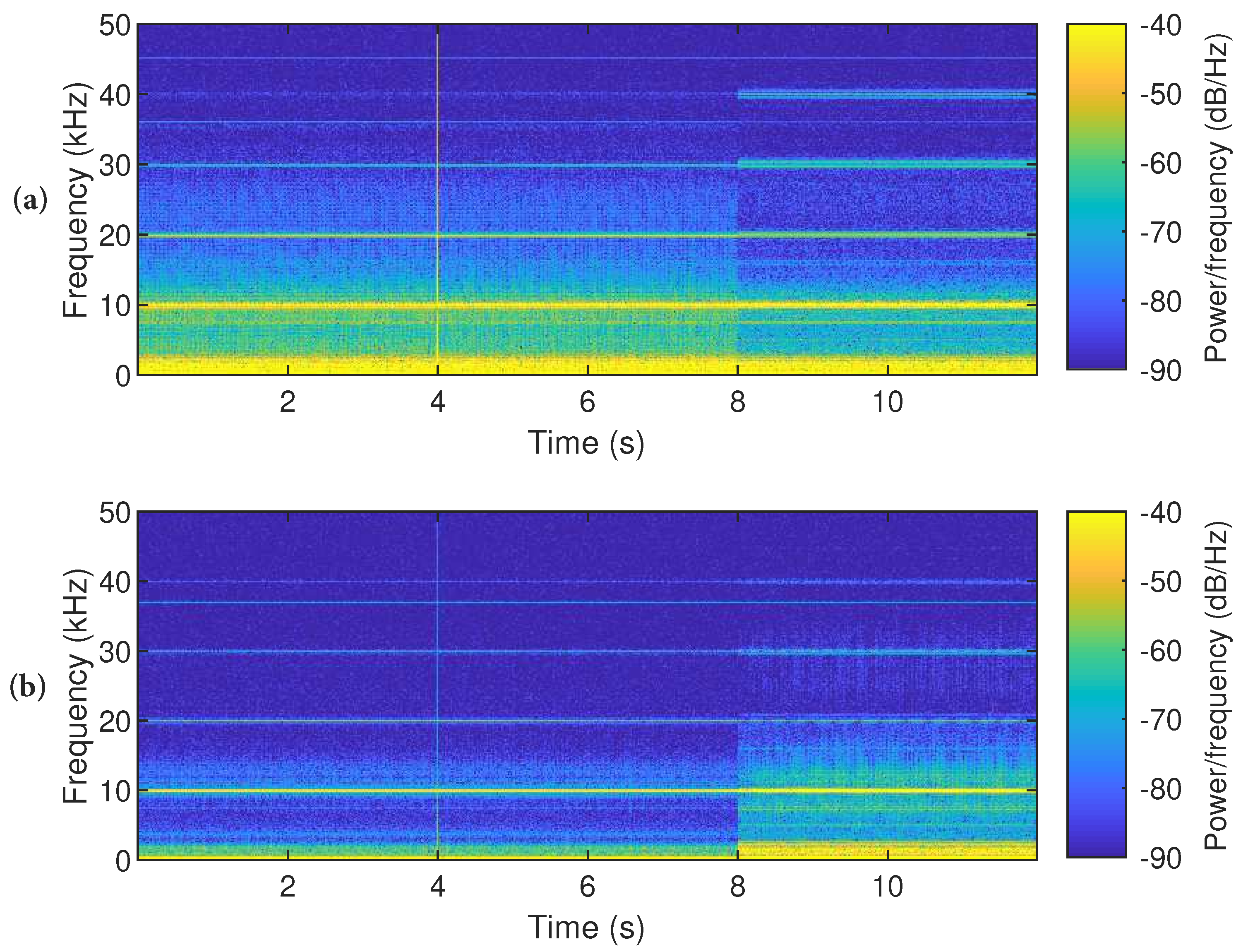
4.2. Emission and Absorption of EV-1 (and EV-3)
For EV-1 and EV-3 (which are of the same type), the spectrum for the different scenarios is shown in
Figure 5 for the lab connected to the grid and in the microgrid. Constant emission around 37 kHz originates from the measurement device. Data files are combined for comparison of the spectra, such that every interval of 4 s represents a new scenario. The time-frequency domain is used for easy comparison of the spectra. The main differences are the background distortion (up to 30 kHz), which reduces for the microgrid and the reduced supraharmonic amplitude when in microgrid operation. In the second interval, EV-2 is connected. This showed no additional supraharmonic emission or absorption of emission from the DUT. Furthermore, in the last interval where EV-3 was connected, the emission increased. This has to do with an effect called “frequency beating” and will be further analyzed and discussed in
Section 5.1.
4.3. Emission and Absorption of EV-2
When analyzing the spectrum of EV-2, the same conclusion is drawn as in
Section 4.2: EV-2 is not emitting (primary emission) nor absorbing (secondary emission) supraharmonic currents from other vehicles. This can be for several reasons. At first, the possibility exists that EV-2 makes use of switching frequencies above the supraharmonic range. This does not necessarily mean that problems are avoided, as the upper limit (150 kHz) is rather arbitrary and does not imply that no conducted disturbances could exist for higher frequencies. Second, the use of filters or other switching configurations can reduce supraharmonic emissions. Neither, however, could be tested or verified.
4.4. Emission and Absorption of EV-4
For EV-4, the same scenarios are used to analyze its supraharmonic emission and absorption. For EV-4, it seems that the emission differs significantly between nominal (full) power and reduced power. In
Figure 6, the first interval shows the spectrum for EV-4 when charging at 16 A. When reducing its power to 14 A, supraharmonic emission between 45 and 49 kHz appears. The emission between 22 and 25 kHz remained constant. For the third interval, EV-3 was added to the setup. A corresponding secondary emission is observed at 10 kHz and its harmonics (20, 30 kHz). The primary emission from EV-4 did not change, but the background emission reduced.
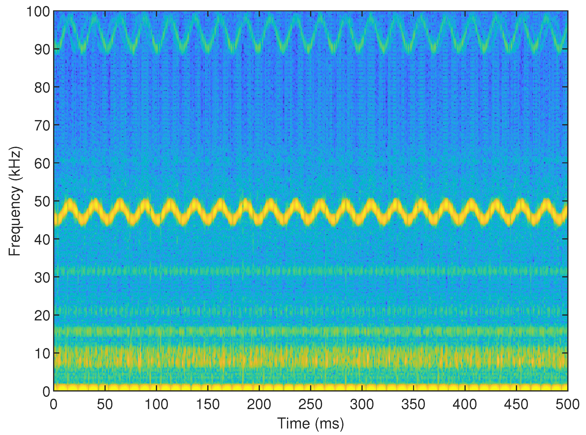
Most converters studied show one narrow-band peak (including its harmonics) in the supraharmonic spectrum. However, EV-4 shows a more broadband emission. Further analysis in the time–frequency domain showed that this device has a periodically changing switching frequency between 45 and 50 kHz. The assumption is that this is the result of making use of boundary conduction mode (BCM) instead of continuous conduction mode (CCM) [
21]. This periodical switching is visible when applying spectral analysis, as shown in
Figure 7, and repeats every 25 ms. Here also, the harmonic component between 90 and 100 kHz is visible. Spreading the emission over a wider spectrum allows the manufacturer to create a lower peak emission. It is, however, still unknown what (additional) effect this has on other equipment connected and the grid and equipment exposed to it. Nevertheless, the broader spectrum results in a higher chance of creating local resonances or other effects because a larger part of the supraharmonic spectrum contains distortion.
4.5. Summary of Results
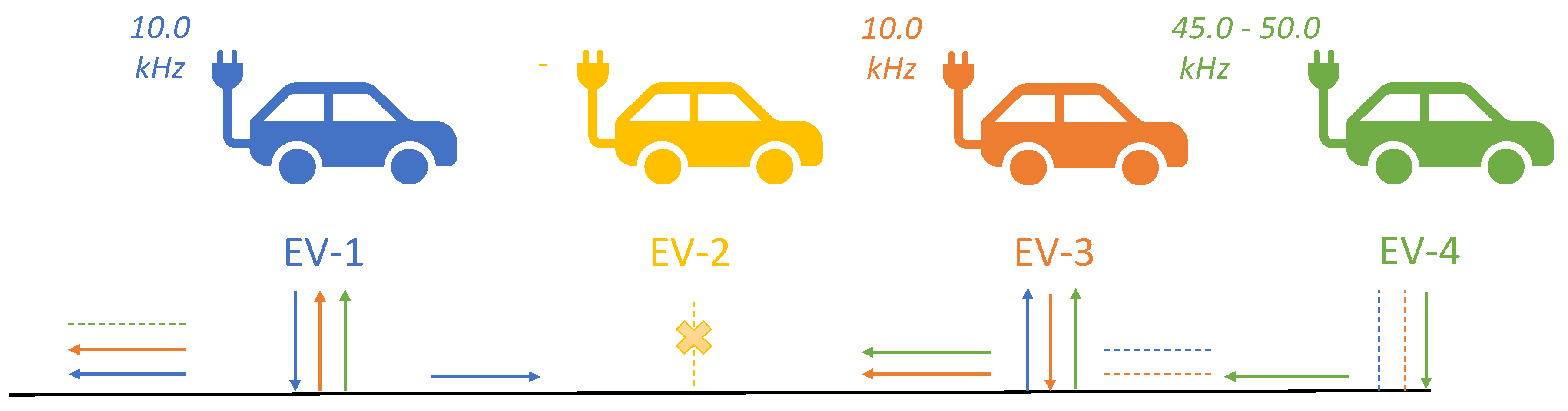
In this section, the most important results and findings from the measurements will be summarized using
Figure 8. In this figure, the 4 tested EVs are shown, with on the top right their supraharmonic emission frequency with the highest amplitude. EV-1 and EV-3 were identical and showed primary narrow-band supraharmonic emission at 10 kHz and its multiples (20 and 30 kHz). EV-2 showed no primary emission within the supraharmonic range. EV-4 had a broadband primary emission between 45 and 50 kHz, and time–frequency analysis showed an oscillating emission with a period of approximately 25 ms.
EV-1, EV-3, and EV-4 absorb emissions from each-other, resulting in secondary emissions and a beating effect between EV-1 and EV-3. The emissions of EV-1 and EV-3 partly flow into the public grid and is influenced by this grid connection. The emission from EV-4 is mainly absorbed by EV-1 and EV-3 and is only slightly influenced by the grid connection. However, the high effect on the voltage at this frequency could indicate local resonance. EV-2 did not absorb any emissions and therefore shows no secondary emissions.
5. Analysis of Supraharmonic Interaction
During the measurements, interaction between EVs was observed. Each subsection will discuss one of these and gives a detailed analysis supported by simulations with MATLAB.
5.1. Frequency Beating
When different devices with the same converter are connected (electrically) close to each other, interaction can occur. Two converters of the same type will never switch at exactly the same frequency, due to impurities in the components and unavoidable flaws in the design process. A slight difference of only 0.01% can cause a difference in switching frequency of the same order. For example, the switching frequency of device A is set at
= 20,000 Hz. Another device of the same type, device B, has a switching frequency that is off by 0.01% of 20,000 Hz;
= 2 Hz. The actual switching frequency is now
= 20,002 Hz. Adding 2 waveforms with a slightly different frequencies will result in varying constructive and destructive parts. This phenomena is called frequency beating and will cause the supraharmonic component to attenuate periodically with a beating frequency directly related to the difference in switching frequencies [
29]:
with
being the observed period of the beating oscillation.
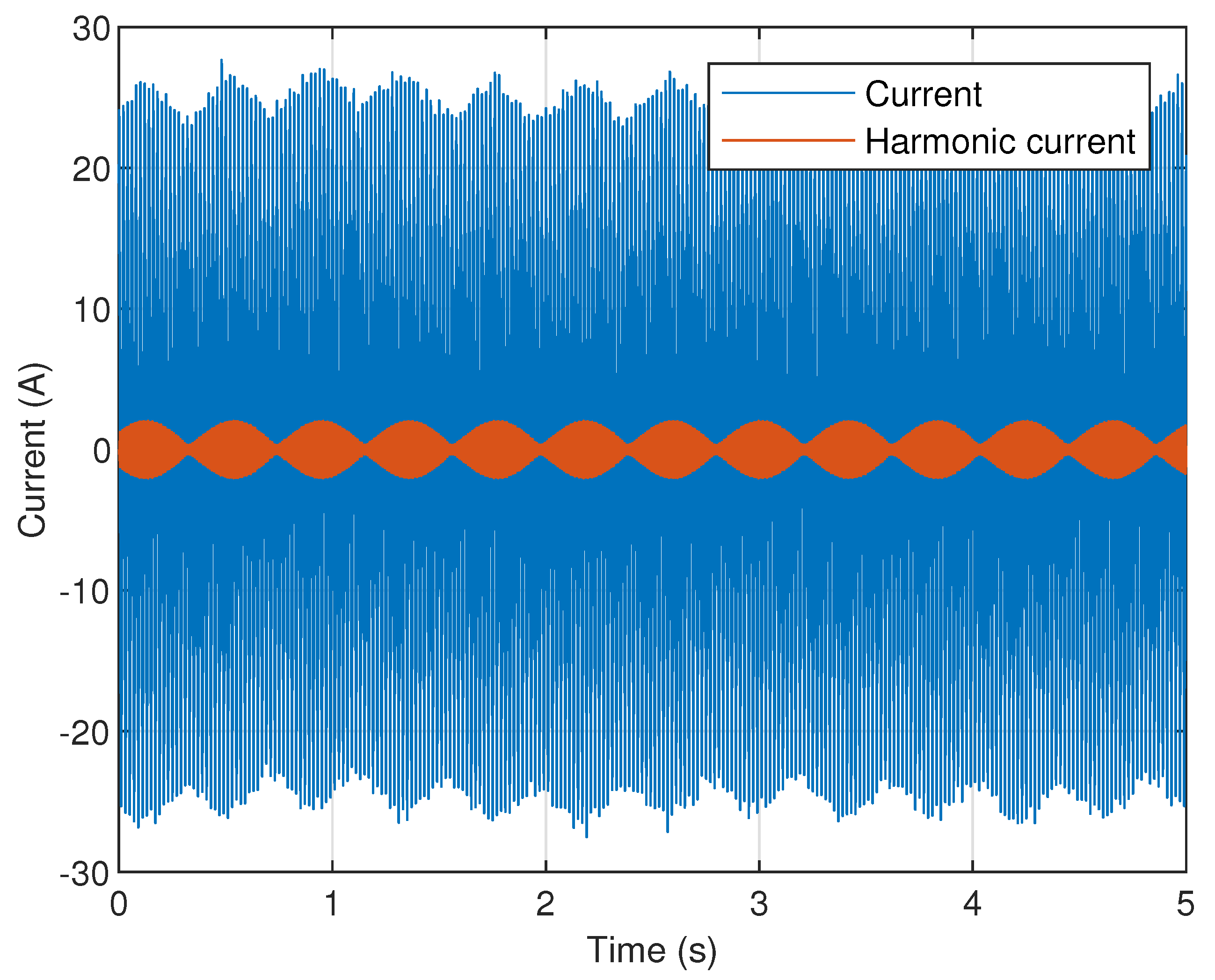
Frequency beating was observed in other measurements at a parking lot with 16 three-phase 22 kW charging stations. When two EVs of the same type were charging, frequency beating was observed. At this location, the residual current devices (RCDs) tripped multiple times a week, especially when 2 or more identical EVs where charging. Supraharmonic currents combined with the described beating effect are the suspected source of the tripping, but this could not be proven. At this location, a supraharmonic component of around 10 kHz was measured, which behaves periodically with a period
of 0.42 s. The frequency difference between the switching frequencies of the two EVs is therefore
= 2.4 Hz. The resulting current waveform as well as the extracted supraharmonic component are shown in
Figure 9. Here, the beating effect is clearly visible in the supraharmonic amplitude that oscillates between −2 and 2 A. In the time–frequency analysis, the beat oscillation is also visible around 10 kHz, see
Figure 10. The amplitude of the higher supraharmonic components (20 and 30 kHz) was too low to determine if a similar beating effect was present.
This effect will have a different periodical behavior when more EVs are added. This was simulated for a combination of three devices with small differences (9999; 10,000; 10,002.4 Hz) in switching frequency, matching the measurements but including another fundamental at 9999 kHz. The result is shown in
Figure 11. Due to the multiple
values that now exist (1, 2.4, 3.4 Hz) the periodic behavior changed.
5.2. Intermodulation Distortion
Another interaction between switching frequencies of devices is intermodulation distortion. Intermodulation occurs when two devices with different switching frequencies of considerable amplitude are connected close to each other. Intermodulation is a different type of distortion than frequency beating because the
is normally in the order of some kHz to tens of kHz, resulting in an additional (supraharmonic) frequency component in the spectrum. Intermodulation is known from communication theory but is also (unintentional) present from the switching artifacts of different converters [
30].
Intermodulation distortion will result in additional frequency components at frequencies related to the two fundamental (supraharmonic) switching frequencies
and
chosen such that
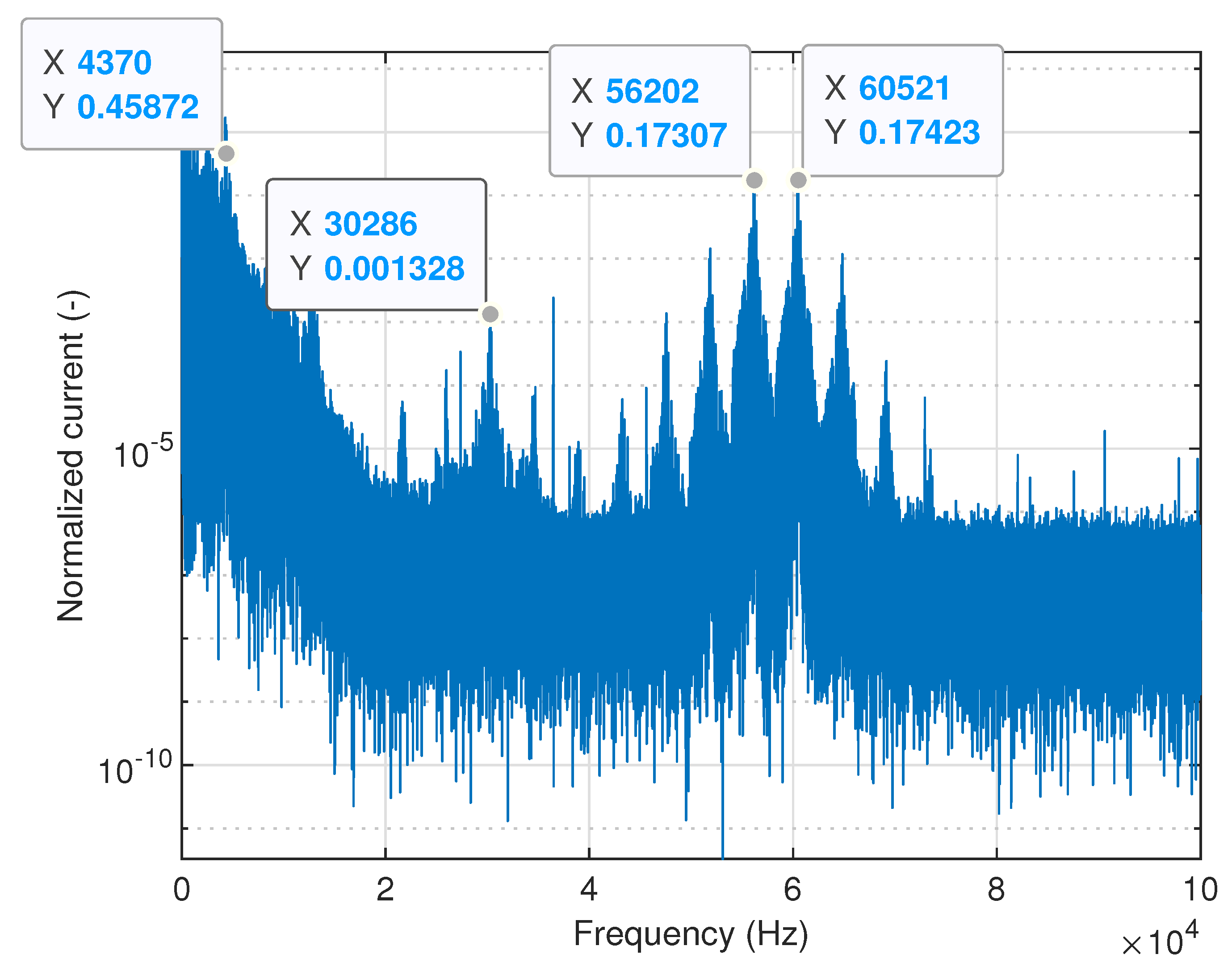
. The measurement shown in
Figure 12 shows intermodulation distortion due to supraharmonic components at
kHz and
kHz. Here, the amplitudes of the current are normalized to the nominal current of the DUT (16 A). Second-order intermodulation is visible at
kHz. Third-order intermodulation distortion is visible at
kHz and
kHz, and even fifth-order intermodulation at
kHz and
kHz. The possibility exists that
originates from a component at
kHz, which is exactly
. This means that the intermodulation distortion in fact originated from a harmonic of
(
) and switching frequency of the EV at
.
This effect was simulated to check whether the given statement matches the theory. For the two components
and
as stated above, the intermodulation components of the 2nd, 3rd, 5th, and 7th order were calculated for both frequency as well as relative amplitude. The result (
Figure 13) shows no component around 30 kHz, which supports the statement that
originates from
and that the component at 4.3 kHz is actually a third-order component from
and
, namely
. This makes this example especially interesting because intermodulation between a harmonic of one of the supraharmonic components also resulted in additional distortion.
6. Conclusions
Research on supraharmonics is increasing, and standards describing supraharmonic emissions are under development. There are a lot of sources of supraharmonics, and this number is expected to increase. Supraharmonics have different effects and can have an influence on devices and grid assets. Most important is the fact that components heat up excessively, influencing the lifetime of equipment. In addition, different interactions can appear when devices are connected close to each other and equipment malfunction or failure is possible.
The goal of this research was to analyze the behavior of supraharmonic emissions from individual EVs and the propagation of supraharmonic currents. Two models were used in order to understand and analyze the propagation of primary harmonic currents to secondary devices and to see the influence of background and other external emissions on secondary emissions from devices. The models are simplified and omit a portion of the interactions between devices that can occur.
A measurement setup and test process were developed to analyze the effects of a single EV, as well as combinations of them. The supraharmonic emissions from individual EVs were measured to obtain spectra of primary emissions. Even though the measurements at frequencies above 20 kHz had a lower accuracy due to the used Rogowski coils, valuable insights were gained. Furthermore, the effect of external emissions on the spectrum was analyzed to study absorption and flows of supraharmonic currents.
Two BEV types (EV-1 and EV-3) were identical and showed narrow-band emissions at 10 kHz and integer multiples. Another BEV (EV-4) showed a broadband emission profile between 45 and 49 kHz. Both absorb harmonic currents from each other (secondary emission). The last BEV (EV-2) showed no primary emission and did not absorb secondary currents from other devices.
Furthermore, the effect of creating a microgrid was studied. The grid connection absorbed a portion of the emissions (from EV-1) and also was a source of additional background emissions. Supraharmonic emissions of EV-1 and EV-3 were influenced by grid connection; the supraharmonic emission from EV-2 and EV-4 remained constant.
Interaction between supraharmonic currents can occur when two devices are connected close to each other. Frequency beating appears with two or more identical devices with a small (some Hz) difference between their fundamental switching frequencies. Intermodulation distortion results in additional supraharmonic components at frequencies related to the fundamental switching frequencies (which differ by some kHz). Broadband emission profiles spread emissions over a wider spectrum with lower peak values by continuously varying the switching frequency. It is unknown whether the described interactions have additional effects on equipment or the grid assets, but one suspected effect is the unwanted tripping of RCDs.
To summarize, the supraharmonic currents from EV-1 and EV-3 propagated between each other, resulting in a beating effect. They also propagated towards EV-4 and were strongly influenced by the grid connection. The emissions from EV-4 were not influenced by the grid connection and mainly propagated towards EV-1 and EV-3. No primary or secondary emissions from EV-2 were measured, and hence, no supraharmonic currents propagated towards or originated from EV-2.
7. Research Limitations and Further Research
In this research, the effect of electric vehicles on supraharmonic propagation in a small (micro)grid was studied. Further research could investigate the effect of higher penetrations of EVs on larger domestic grids and could also include the effect of PV and other types of EV chargers with higher power (DC fast chargers). In addition, the effect of intentional emission as used for PLC can be studied further. This will give more representative insight into propagation to and emission from households.
The currents towards the grid were not measured in the lab due to safety restrictions. Indicative measurements at a parking lot with 15 charging points showed that most emissions propagate between the EVs and only a small portion flows back into the grid. Of interest is whether the same applies for other parking lots and for a domestic grid.
On a higher power level, DC fast chargers (at the moment up to 350 kW but expected to increase towards 1 MW) will be sources of supraharmonic emissions as well, shown in indicative measurements by the authors. Of interest is the supraharmonic emissions of these device and the impact on the grid.
Supraharmonic currents are potentially transferred by a distribution transformer from an LV to a medium-voltage (MV) grid. This depends on the transformer and cables used and the strength of the MV grid upstream. The mentioned fast chargers are mainly connected by dedicated LV cables directly to a (dedicated) transformer (in future, possibly directly to the MV grid). Further research could investigate how realistic a transfer of supraharmonic currents from the LV to the MV grid is in practice and whether it propagates through the MV grid as well, potentially affecting other downstream LV grids.
Harmonic load flow and summation models only describe part of the physics behind supraharmonic propagation and emission. Supraharmonic interaction is also not taken into account here. For grid planning and operation, it would be useful to include the effects of supraharmonics and to make a prediction of future severity and measures needed. This is difficult because this depends on (mainly uncontrollable) variables.
Author Contributions
Conceptualization, T.S. and V.Ć.; methodology, T.S. and S.C.; validation, T.S. and V.Ć.; formal analysis, T.S.; investigation, T.S. and T.v.W.; resources, T.v.W.; data curation, T.S.; writing—original draft preparation, T.S.; writing—review and editing, T.v.W., V.Ć., and S.C.; visualization, T.S. and T.v.W.; supervision, S.C. All authors have read and agreed to the published version of the manuscript.
Funding
This research received no external funding.
Acknowledgments
Thanks to The Smart Grid Interoperability Laboratory (SGIL) of the Joint Research Centre (European Commission) in Petten for helping to facilitate this research.
Conflicts of Interest
The authors declare no conflict of interest.
Abbreviations
The following abbreviations are used in this manuscript:
| BEV | battery or full electric vehicle |
| DAQ | data acquisition |
| DUT | device under test |
| EMC | electromagnetic compatibility |
| EV | electric vehicle in general. Used for indexing. |
| LV | low voltage |
| MV | medium voltage |
| PCC | point of common coupling |
| PLC | power line communication |
| PV | photo-voltaic |
| SGIL | smart-grid interoperability lab |
References
- Yu, B.; Guo, J.; Zhou, C.; Gan, Z.; Yu, J.; Lu, F. A Review on Microgrid Technology with Distributed Energy. In Proceedings of the 2017 International Conference on Smart Grid and Electrical Automation (ICSGEA), Changsha, China, 27–28 May 2017; pp. 143–146. [Google Scholar] [CrossRef]
- Schmitt, L.; Kayal, S.; Kumar, J. Microgrids and the future of the European city. In Proceedings of the 2014 Saudi Arabia Smart Grid Conference (SASG), Jeddah, Saudi Arabia, 15–17 December 2014; pp. 1–3. [Google Scholar] [CrossRef]
- Ronnberg, S.K.; Castro, A.G.d.; Bollen, M.H.; Moreno-Munoz, A.; Romero-Cadaval, E. Supraharmonics from power electronics converters. In Proceedings of the 2015 9th International Conference on Compatibility and Power Electronics (CPE), Costa da Caparica, Portugal, 24–26 June 2015; pp. 539–544. [Google Scholar] [CrossRef]
- Moreno-Munoz, A.; Gil-de Castro, A.; Romero-Cavadal, E.; Ronnberg, S.; Bollen, M. Supraharmonics (2 to 150 kHz) and multi-level converters. In Proceedings of the 2015 IEEE 5th International Conference on Power Engineering, Energy and Electrical Drives (POWERENG), Riga, Latvia, 11–13 May 2015; pp. 37–41. [Google Scholar] [CrossRef]
- Meyer, J.; Khokhlov, V.; Klatt, M.; Blum, J.; Waniek, C.; Wohlfahrt, T.; Myrzik, J. Overview and Classification of Interferences in the Frequency Range 2–150 kHz (Supraharmonics). In Proceedings of the 2018 International Symposium on Power Electronics, Electrical Drives, Automation and Motion (SPEEDAM), Amalfi, Italy, 20–22 June 2018; pp. 165–170. [Google Scholar] [CrossRef]
- Rönnberg, S.K.; Bollen, M.H.; Amaris, H.; Chang, G.W.; Gu, I.Y.; Kocewiak, Ł.H.; Meyer, J.; Olofsson, M.; Ribeiro, P.F.; Desmet, J. On waveform distortion in the frequency range of 2 kHz–150 kHz—Review and research challenges. Electr. Power Syst. Res. 2017, 150, 1–10. [Google Scholar] [CrossRef]
- International Energy Agency. Global EV Outlook; International Energy Agency: Paris, France, 2019. [Google Scholar]
- Meyer, J.; Mueller, S.; Ungethuem, S.; Xiao, X.; Collin, A.; Djokic, S. Harmonic and supraharmonic emission of on-board electric vehicle chargers. In Proceedings of the 2016 IEEE PES Transmission & Distribution Conference and Exposition-Latin America (PES T&D-LA), Morelia, Mexico, 2–5 May 2016; pp. 1–7. [Google Scholar] [CrossRef]
- Schottke, S.; Meyer, J.; Schegner, P.; Bachmann, S. Emission in the frequency range of 2 kHz to 150 kHz caused by electrical vehicle charging. In Proceedings of the 2014 International Symposium on Electromagnetic Compatibility, Gothenburg, Sweden, 1–4 September 2014; pp. 620–625. [Google Scholar] [CrossRef]
- Collin, A.J.; Djokic, S.Z.; Thomas, H.F.; Meyer, J. Modelling of electric vehicle chargers for power system analysis. In Proceedings of the 11th International Conference on Electrical Power Quality and Utilisation, Lisbon, Portugal, 17–19 October 2011; pp. 1–6. [Google Scholar] [CrossRef]
- Xiao, X.; Molin, H.; Kourtza, P.; Collin, A.; Harrison, G.; Djokic, S.; Meyer, J.; Muller, S.; Moller, F. Component-based modelling of EV battery chargers. In Proceedings of the 2015 IEEE Eindhoven PowerTech, Eindhoven, The Netherlands, 29 June–2 July 2015; pp. 1–6. [Google Scholar] [CrossRef]
- Horton, R.; Taylor, J.A.; Maitra, A.; Halliwell, J. A time-domain model of a plug-in electric vehicle battery charger. In Proceedings of the PES T&D 2012, Orlando, FL, USA, 7–10 May 2012; pp. 1–5. [Google Scholar] [CrossRef]
- Cassano, S.; Silvestro, F.; Jaeger, E.D.; Leroi, C. Modeling of harmonic propagation of fast DC EV charging station in a Low Voltage network. In Proceedings of the 2019 IEEE Milan PowerTech, Milan, Italy, 23–27 June 2019; p. 6. [Google Scholar]
- Espin-Delgado, A.; Ronnberg, S.; Busatto, T.; Ravindran, V.; Bollen, M. Summation Law for Supraharmonic Currents (2 to 150 kHz) in Low-Voltage Installations. Electr. Power Syst. Res. 2019, 184, 106325. [Google Scholar] [CrossRef]
- Bollen, M.; Olofsson, M.; Larsson, A.; Ronnberg, S.; Lundmark, M. Standards for supraharmonics (2 to 150 kHz). IEEE Electromagn. Compat. Mag. 2014, 3, 114–119. [Google Scholar] [CrossRef]
- Bollen, M.; Ronnberg, S. Propagation of Supraharmonics in the Low Voltage Grid; Energiforsk: Stockholm, Sweden, 2017. [Google Scholar]
- Larsson, E.O.A.; Bollen, M.H.J. Emission and immunity of equipment in the frequency range 2 to 150 kHz. In Proceedings of the 2009 IEEE Bucharest PowerTech, Bucharest, Romania, 28 June–2 July 2009; pp. 1–5. [Google Scholar] [CrossRef]
- Arechavaleta, M.; Halpin, S.M.; Birchfield, A.; Pittman, W.; Griffin, W.E.; Mitchell, M. Potential Impacts of 9–150 kHz Harmonic Emissions on Smart Grid Communications in the United States. In Proceedings of the ENERGY 2015: The Fifth International Conference on Smart Grids, Green Communications and IT Energy-aware Technologies, Rome, Italy, 24–29 May 2015; p. 6. [Google Scholar]
- Meyer, J.; Haehle, S.; Schegner, P. Impact of higher frequency emission above 2kHz on electronic mass-market equipment. In Proceedings of the 22nd International Conference and Exhibition on Electricity Distribution (CIRED 2013), Stockholm, Sweden, 10–13 June 2013. [Google Scholar] [CrossRef]
- Waniek, C.; Wohlfahrt, T.; Myrzik, J.M.; Meyer, J.; Schegner, P. Topology identification of electronic mass-market equipment for estimation of lifetime reduction by HF disturbances above 2 kHz. In Proceedings of the 2017 IEEE Manchester PowerTech, Manchester, UK, 18–22 June 2017; pp. 1–6. [Google Scholar] [CrossRef]
- Waniek, C.; Wohlfahrt, T.; Myrzik, J.M.; Meyer, J.; Klatt, M.; Schegner, P. Supraharmonics: Root causes and interactions between multiple devices and the low voltage grid. In Proceedings of the 2017 IEEE PES Innovative Smart Grid Technologies Conference Europe (ISGT-Europe), Torino, Italy, 23–26 April 2017; pp. 1–6. [Google Scholar] [CrossRef]
- Slangen, T.M.H.; van Wijk, T.; Cuk, V.; Cobben, J.F.G. The Harmonic and Supraharmonic Emission of Battery Electric Vehicles in The Netherlands. In Proceedings of the 2020 International Conference on Smart Energy Systems and Technologies (SEST), Istanbul, Turkey, 7–9 September 2020; p. 6. [Google Scholar]
- Ronnberg, S.; Larsson, A.; Bollen, M. A Simple Model for Interaction Between Equipment at a Frequency of Some Tens of kHz. In Proceedings of the International Conference on Electricity Distribution, Frankfurt, Germany, 6–9 June 2011; p. 4. [Google Scholar]
- Hayt, W. Engineering Electromagnetics; Number 8th; McGraw-Hill Education: New York, NY, USA, 2010. [Google Scholar]
- Schottke, S.; Rademacher, S.; Meyer, J.; Schegner, P. Transfer characteristic of a MV/LV transformer in the frequency range between 2 kHz and 150 kHz. In Proceedings of the 2015 IEEE International Symposium on Electromagnetic Compatibility (EMC), Dresden, Germany, 16–22 August 2015; pp. 114–119. [Google Scholar] [CrossRef]
- Korner, P.M.; Stiegler, R.; Meyer, J.; Wohlfahrt, T.; Waniek, C.; Myrzik, J.M. Acoustic noise of massmarket equipment caused by supraharmonics in the frequency range 2 to 20 kHz. In Proceedings of the 2018 18th International Conference on Harmonics and Quality of Power (ICHQP), Ljubljana, Slovenia, 29–30 March 2018; pp. 1–6. [Google Scholar] [CrossRef]
- Jiang, L.; Ye, G.; Xiang, Y.; Cuk, V.; Cobben, J. Influence of high frequency current harmonics on (Smart) energy meters. In Proceedings of the 2015 50th International Universities Power Engineering Conference (UPEC), Stoke On Trent, UK, 1–4 September 2015; pp. 1–5. [Google Scholar] [CrossRef]
- Sakar, S.; Ronnberg, S.; Bollen, M. Interferences in AC–DC LED Drivers Exposed to Voltage Disturbances in the Frequency Range 2–150 kHz. IEEE Trans. Power Electron. 2019, 34, 11171–11181. [Google Scholar] [CrossRef]
- Yue, X.; Boroyevich, D.; Lee, F.C.; Chen, F.; Burgos, R.; Zhuo, F. Beat Frequency Oscillation Analysis for Power Electronic Converters in DC Nanogrid Based on Crossed Frequency Output Impedance Matrix Model. IEEE Trans. Power Electron. 2018, 33, 3052–3064. [Google Scholar] [CrossRef]
- Abid, F.; Busatto, T.; Ronnberg, S.K.; Bollen, M.H.J. Intermodulation due to interaction of photovoltaic inverter and electric vehicle at supraharmonic range. In Proceedings of the 2016 17th International Conference on Harmonics and Quality of Power (ICHQP), Belo Horizonte, Brazil, 16–19 October 2016; pp. 685–690. [Google Scholar] [CrossRef]
Figure 1.
A simple model describing primary and secondary emission. Primary emission from device 1 is denoted as , of which a part results in the secondary emission of device 2 (), depending on the impedance ratio. The total emission of device 2 is now composed of its own primary emission superimposed on the secondary emission from device 1.
Figure 2.
Measured current of a single-phase battery electric vehicle charging at 16 Arms with supraharmonic distortion at 10 kHz. The amplitude of the supraharmonic component is approximately 1 A (5% of the fundamental) and also results in an effect on the voltage (approximately 1 Vpp).
Figure 2.
Measured current of a single-phase battery electric vehicle charging at 16 Arms with supraharmonic distortion at 10 kHz. The amplitude of the supraharmonic component is approximately 1 A (5% of the fundamental) and also results in an effect on the voltage (approximately 1 Vpp).
Figure 3.
Simple model describing the flow of harmonic currents from a single device () towards its internal impedance and towards other external impedances , the inverter impedances and , and the grid . The external emission is denoted as . Device and grid impedances are not constant over frequency, changing the harmonic load flow for different frequencies and sources.
Figure 4.
Simplified schematic overview of the lab that can either work as a microgrid or be connected to the public grid. From top to bottom, on the left: 33 × 250 Wp PV panels with a 3-phase PV inverter (8 kW total), 1600 Ah 48 V (76 kWh) lead acid batteries with multiple 1-phase inverters (30 kW total), public grid connection (switchable). On the right: base load from lab (LED, servers), four 11 or 22 kW (3-phase) electric vehicle (EV) charging stations.
Figure 5.
Time–frequency analysis of current emission of EV-1. First interval (0–4 s): only EV-1; second interval (4–8 s): EV-1 and EV-2; third interval (8–12 s): EV-1, EV-2, and EV-3. For grid connection (a), the emission of EV-1 is higher compared to microgrid (b) operation. The effect of adding EV-2 is insignificant. Adding EV-3 increases the amplitude and results in a beating effect.
Figure 6.
Time–frequency analysis of emission from EV-4. The first interval (0–4 s) shows only EV-4 at nominal power, second interval (4–8 s) shows EV-4 at reduced power, and the third interval (8–12 s) shows EV-4 at reduced power and the absorbed secondary emission of EV-3. For public grid connection (a) and microgrid operation (b), the emissions are similar.
Figure 7.
Time–frequency analysis of broadband supraharmonic emission EV-4. The emission frequency is time-dependent and oscillates between 45 and 50 kHz. The period of oscillation is approximately 25 ms. A harmonic of this oscillating component is visible between 90 and 100 kHz.
Figure 7.
Time–frequency analysis of broadband supraharmonic emission EV-4. The emission frequency is time-dependent and oscillates between 45 and 50 kHz. The period of oscillation is approximately 25 ms. A harmonic of this oscillating component is visible between 90 and 100 kHz.
Figure 8.
Overview of results on supraharmonic emission and propagation.
Figure 8.
Overview of results on supraharmonic emission and propagation.
Figure 9.
Measured current with beating effect and extracted supraharmonic currents around 10 kHz. Due to a of 2.4 Hz between the switching frequencies of two identical EVs, a periodical beating effect with a period of 0.42 s appears in the current taken by this EV.
Figure 9.
Measured current with beating effect and extracted supraharmonic currents around 10 kHz. Due to a of 2.4 Hz between the switching frequencies of two identical EVs, a periodical beating effect with a period of 0.42 s appears in the current taken by this EV.
Figure 10.
Time–frequency analysis of the measured beating effect around 10 kHz. The oscillating behavior of the supraharmonic components around 10 kHz is visible. Furthermore, distortion around 20 and 30 kHz is observed with a lower amplitude but with the beating effect present to a certain extent as well.
Figure 11.
Simulated beating effect for 3 EVs with small differences between switching frequencies ( = 9999, = 10,000, and = 10,002.4 Hz) and extracted supraharmonic currents. The beating pattern is dependent on the number of devices and their individual values. The frequencies are chosen such that they are representative of 3 identical EVs with small differences in switching frequencies, similar to previous results.
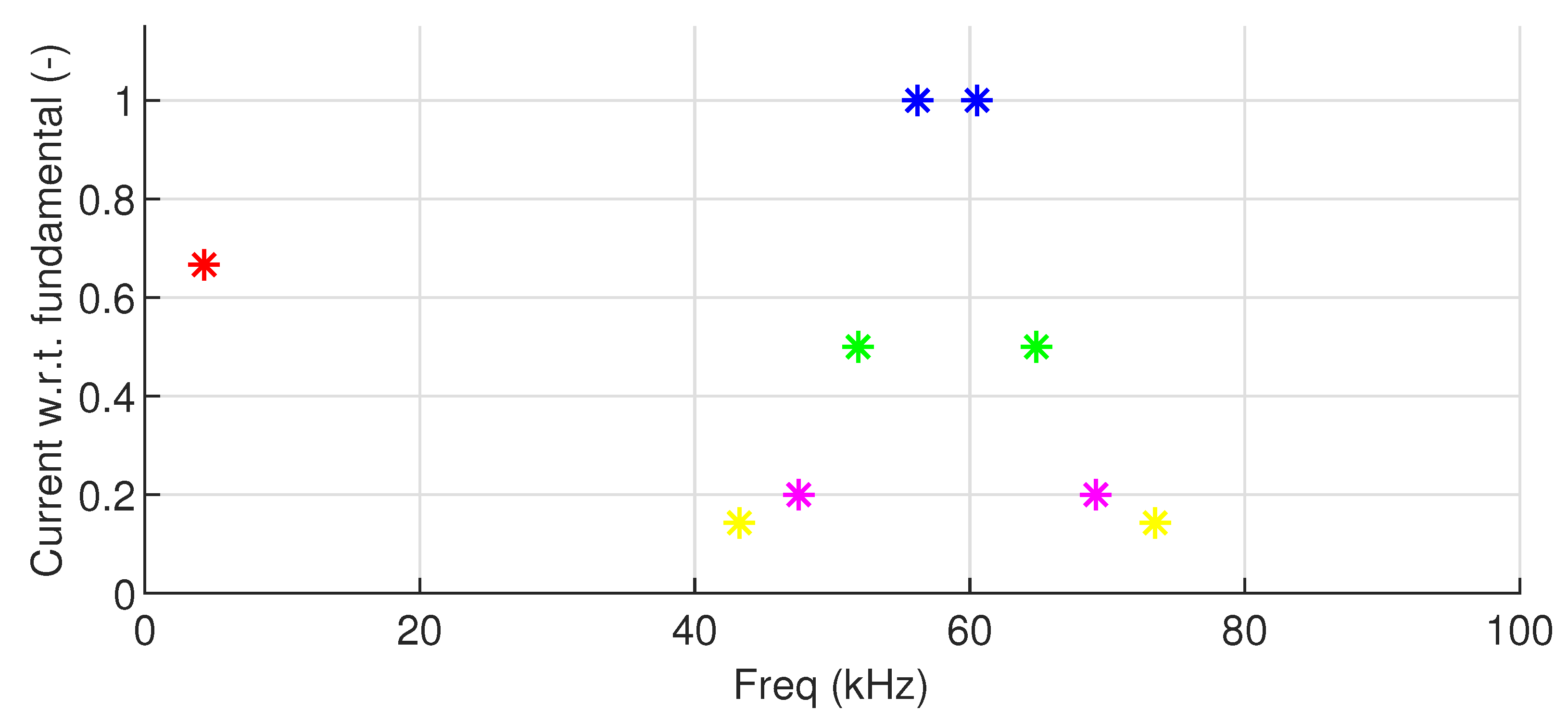
Figure 12.
Frequency analysis of measured intermodulation current distortion as a result of two supraharmonic components and at 56.2 and 60.5 kHz, respectively. Second-order intermodulation is visible at kHz, and third-order intermodulation at kHz and kHz. The component at 60.5 kHz is possibly a harmonic of the component at 30.2 kHz.
Figure 13.
Simulated intermodulation current distortion for kHz and kHz, up to the 7th order. No component at 30.2 kHz is visible now, which supports the statement that the 60.5 kHz component could be a harmonic of the 30.2 kHz component.
Figure 13.
Simulated intermodulation current distortion for kHz and kHz, up to the 7th order. No component at 30.2 kHz is visible now, which supports the statement that the 60.5 kHz component could be a harmonic of the 30.2 kHz component.
Table 1.
Data on the different battery electric vehicles used for testing. EV-1 and EV-3 are of the same type. For combined tests, the maximum power was reduced to 11 kW per charging station.
Table 1.
Data on the different battery electric vehicles used for testing. EV-1 and EV-3 are of the same type. For combined tests, the maximum power was reduced to 11 kW per charging station.
| Max. Current
Per Phase (A) | Nr. of Phases | Max. Power
(kW) | Battery Capacity
(kWh) |
|---|
| EV-1/EV-3 | 32 | 3 | 22 | 52 |
| EV-2 | 29 | 1 | 6.7 | 36 |
| EV-4 | 16 | 3 | 11 | 64 |
Table 2.
Comparison of supraharmonic current emission and effect on the voltage at different frequencies of interest when charging at 16 A. Results for the lab connected to the public grid (left) and for the lab in microgrid operation (right) are shown. Especially the emissions of EV-1 (and EV-3) at 10 kHz (shown in bold) are significantly affected by the operation mode. In the microgrid, the emission as well as the effect on the voltage was approximately halved. For the emission of EV-4 at 45–50 kHz (also shown in bold), the effect of the voltage is large, possibly due to a local resonance at this frequencies. EV-2 is left out of these results.
| | Public Grid | Microgrid |
|---|
| Frequency
(kHz) | Emission () | Voltage (V) | Emission () | Voltage (V) |
|---|
| EV-1/EV-3 | 10 | 1.761 | 1.305 | 0.865 | 0.699 |
| EV-1/EV-3 | 20 | 0.083 | 0.141 | 0.040 | 0.059 |
| EV-1/EV-3 | 30 | 0.011 | 0.047 | 0.014 | 0.040 |
| EV-4, 14 A | 45–50 | 0.205 | 1.067 | 0.225 | 1.037 |
| EV-4 | 45–50 | 0.004 | 0.045 | 0.005 | 0.037 |
© 2020 by the authors. Licensee MDPI, Basel, Switzerland. This article is an open access article distributed under the terms and conditions of the Creative Commons Attribution (CC BY) license (http://creativecommons.org/licenses/by/4.0/).


