Abstract
In practical power system operation, knowing the voltage stability limits of the system is important. This paper proposes using a decision tree (DT) to extract guidelines through offline study results for assessing system voltage stability status online. Firstly, a sample set of DTs is determined offline by active power injection and bus voltage magnitude (P-V) curve analysis. Secondly, participation factor (PF) analysis and the Relief-F algorithm are used successively for attribute selection, which takes both the physical significance and the classification capabilities into consideration. Finally, the C4.5 algorithm is used to build the DT because it is more suitable for handling continuous variables. A practical power system is implemented to verify the feasibility of the proposed online voltage stability margin (VSM) assessment framework. Study results indicate that the operating guidelines extracted from the DT can help power system operators assess real time VSM effectively.
1. Introduction
Voltage stability refers to the capability of maintaining voltage within safe or acceptable limits, even in the case of credible contingencies [1,2,3,4]. Current industry practice is to perform offline voltage stability studies and extract operating guidelines to monitor and control the system state. Due to the interconnections of power systems, the scale of the power grid expands rapidly and operating conditions become more complicated. Furthermore, due to the rapid development of wind power and photovoltaic power generation in the power grid, greater uncertainty has been introduced. To investigate system stability limits, operational planners have to perform more offline studies of various system topologies and conditions. Data collected from these offline studies has reached an unprecedented level. Currently, individual operational planners analyze offline data manually or semi-automatically. Each individual is only capable of exploring valuable information from small amounts of data and is unable to manually process large amounts of data. Determination of stability limits is dependent on an individual operational planner’s experience and knowledge, which is inevitably limited and fragmentary. Although online voltage stability analysis has been implemented by some utilities, it remains a challenge to extract useful information from the mass of data obtained from voltage stability analysis results within an operating time frame.
Data mining techniques provide opportunities to solve this problem, as they can process large amounts of data automatically and efficiently. Researchers have applied data mining technologies, such as artificial neural networks (ANNs), support vector machine (SVMs), and naive Bayes (NB) algorithms, and various improved versions, to online voltage stability assessment [5,6,7,8,9,10,11,12,13,14,15,16,17,18,19,20,21,22,23,24,25,26,27,28,29]. However, these attempts use black box models, which hide the inner data mining process and cannot extract underlying valuable information [30].
Decision trees (DTs) are easier to understand and explain than black-box models because of their tree-like structure. They both reveal the inner data mining process and achieve a precise assessment [31]. References [32,33,34,35,36] proposed using a classification and regression tree (CART) algorithm for voltage stability assessment. Reference [32] scored the full paths of a DT rather than the classification results stored in leaf nodes to assess voltage stability. Reference [33] constructed a regularly updated DT for the voltage stability problem. Reference [35] applied a DT to assess voltage stability and discussed the influence of the DT growing method on classification accuracy. Each of these methods constructed DTs with the CART algorithm, which computes the Gini index to determine the most suitable attribute for purifying a sample set and then builds a binary tree from top to bottom [37]. However, a restriction of the CART algorithm is that it cannot effectively handle continuous attributes. Because voltage amplitude, reactive power of generators and that of branches are continuous variables, system operators need an exact value to assess the system voltage stability status. When handling continuous attributes, the CART algorithm discretizes data into several intervals. According to these intervals, the classification boundary is determined. Therefore, the DT can provide inaccurate reference values on leaf nodes. The assessment results may be incorrect after several judgements and lead operators to make a wrong decision.
Previous research divided voltage stability status into two categories, voltage stable and voltage unstable, and applied the decision tree for classification [38,39,40,41,42,43]. Reference [39] employed the CART and C4.5 algorithms to build DTs, and combined the bagging and adaptive boosting methods to increase accuracy. Reference [41] presented a Hoeffding tree method for the voltage security problem. Reference [43] applied the relief and C4.5 algorithms to construct a DT to evaluate the system state. However, even if the voltage instability status can be identified accurately, there is not enough time for system operators to take remedial action. In practical system operation, it is important to know the current operating point and the distance to voltage instability. Therefore, there is a pressing need to perform online voltage stability margin (VSM) assessment. This paper considers the actual demands of online VSM assessment and presents the use of a DT to extract guidelines to help operators to evaluate power system state.
2. Theoretical Framework
This section is composed of three parts. First, the sample set is established for the DT. According to the P-V curve analysis, the VSM is determined and the DT’s sample set then can be generated. Second, participation factor (PF) analysis and the Relief-F algorithm are sequentially applied in attribute selection. Finally, the DT is built using the C4.5 algorithm for online VSM assessment.
2.1. Establish Sample Set for DT
For each network topology, the maximum power transfer point is obtained by gradually increasing system loads with the original operating point. Once it is reached, VSM can be determined and corresponding training samples then can be generated.
The variation of voltage amplitude V with active power P is plotted as the P-V curve. The system VSM is given as follows:
where is active power of the ith operating point. represents the active power of the maximum power transfer point.
In practice, system operators usually avoid operating the power system in the region below the maximum power transfer point. According to monitoring needs, operators usually divide the system into three states: normal state, alert state, and emergency state.
Table 1 shows these three system states and their corresponding VSM.

Table 1.
Voltage stability status.
When is within the interval [5%, 8%), the power system is considered to be at a normal state. The operating points within this interval are treated as normal samples and assigned with class label N. In a similar vein, the alert samples and emergency samples are selected and assigned with class label A and class label E, respectively. If the number of a certain class of samples is much smaller than that of others, this class of samples may be mistaken for noise. In the classifying process, the DT may neglect learning these samples, which means the DT cannot learn the true structure of data. This is called “underfitting” [37]. In system operation, operators tend to focus more on the emergency state. However, the number of emergency samples is obviously less than that of normal or alert samples. Therefore, the same number of samples should be selected from each class for constructing the sample set to avoid underfitting.
2.2. Determine Attributes for the DT
First, modal analysis is implemented for distinguishing pivotal voltage stability modes. For each pivotal mode, PF analysis is applied for selecting attributes preliminarily. Second, the relief-F algorithm is used for further selecting attributes and the final attribute set then can be determined for DT.
The relationship of reactive power increment to voltage amplitude increment is expressed using the following equation [1,2]:
where represents the reduced Jacobian matrix. and are incremental changes in voltage amplitude and reactive power, respectively.
The ith modal voltage change is calculated as follows:
where is the ith eigenvalue of . is the modal reactive power change. It is clear that if , a slight change in will cause significant changes in . The system is considered to be on the brink of voltage instability if one of the eigenvalues equals 0.
The eigenvalues are obtained using eigenvalue analysis based on P-V curves. The smallest eigenvalue, which can be used for measuring the distance to voltage instability, is chosen to implement PF analysis.
The PF at bus k of mode i is shown as:
where and are kth elements of the ith column right eigenvector and ith row left eigenvector of , respectively.
According to (4), the PFs of each bus are calculated and the buses are listed in descending order based on the bus PF analysis results. The differences between adjacent PFs then can be calculated and the largest is regarded as the threshold. The bus whose PF is above the threshold is selected as the key bus.
The branch PF of branch j in mode i is given as:
where and are reactive power loss of branch j and the maximum loss in all branches, respectively.
The generation PF is given as:
where and are reactive power loss of generator k and the maximum loss of all generators, respectively.
The corresponding key branches and generators can be determined in a similar way to key buses. The voltage amplitude and voltage phase angle of buses, reactive power of branches, and reactive power of generators comprise the DT’s initial attributes.
PF analysis can effectively identify which buses, branches, or generators are important to voltage stability. However, these initial attributes may not have good classification capability. If an attribute is closely correlated with another attribute, these two attributes have the same classification capability. One of these two attributes can be regarded as redundant. In addition, some attributes are irrelevant attributes that may not be useful for classification. If many redundant attributes and/or irrelevant attributes are chosen, the DT is larger than necessary [37,44]. Initial attributes determined by PF analysis should be further selected from a classification capability perspective.
Relief algorithms, one of the most successful preprocessing algorithms, can select attributes effectively without any assumption of attribute independence. However, they are restricted to two-class problems [45,46,47,48,49]. The Relief-F algorithm, which is extended from the relief algorithm and suitable for handling multi-class problems, is applied in this paper to further select attributes. The core of the algorithm is to compute weight values iteratively for attributes based on the distance of different samples. At the beginning, sample is selected randomly. From the same class with sample , m nearest neighbors, which are represented by , are selected. In addition, the m nearest neighbors, which are represented by , from each of the different classes is also selected. The weight of attribute A is given as:
where is the weight value of attribute A. n represents the number of iterations. represents the probability of samples belonging to class C. diff represents the difference between and or under attribute A:
where and are the values of sample and of attribute A, respectively. and are the maximum and minimum values, respectively, of attribute A for all of the samples.
For attribute A, if is larger than , then the attribute is suitable for dividing the sample set and the weight value should be raised.
According to (7), the weight value of each attribute can be obtained and then listed in descending order. The threshold value is determined based on the most obvious change between adjacent weight values. Given that the attributes with larger weight values have a more positive effect on classification, the attributes whose weight values are greater than the threshold value are selected.
2.3. Apply C4.5 Algorithm to Build DT
The tree-like structure of the DT reveals the classification rules visually. Once the DT is constructed, a series of operating guidelines are obtained for operators to monitor system voltage stability status.
CART, Iterative Dichotomiser 3 (ID3), and C4.5 are commonly used algorithms to construct DTs. The C4.5 algorithm is better suited to handling continuous attributes than the CART algorithm and can avoid the overfitting problem of the ID3 algorithm [50]. The C4.5 algorithm comprises four main steps. First, the initial information entropy of the sample set is calculated. Second, the split entropy of the sample set under a selected attribute is calculated. Then the information gain can be easily obtained by subtracting the split entropy from the initial information entropy. Finally, the information gain ratio corresponding to the selected attribute is calculated based on the information gain.
2.3.1. Calculate the Initial Information Entropy
2.3.2. Calculate the Split Entropy
Assume that S is divided into two subsets by a randomly selected attribute A. The split entropy is shown as follows:
where and are subsets of S. , and represent the number of samples in each set.
2.3.3. Obtain the Information Gain
The information gain is calculated to quantify the ability of attributes to reduce the overall entropy:
However, if the information gain is regarded as the attribute selection criterion of the DT, it may result in overfitting.
2.3.4. Calculate the Information Gain Ratio
Split information is introduced to solve the overfitting problem, which is calculated using the following equation:
A greater information gain ratio means a better attribute. The most suitable attribute of each node can be identified by calculating the information gain ratio for each attribute recursively. The branches of the DT are the system voltage stability guidelines, which can be extracted for operators to identify the system state.
The C4.5 algorithm can only access the generated sample set. The error computed in this process is the training error. However, an excellent DT must not only fit the generated sample set well, but also classify the unknown samples accurately. The expected error of previously unknown samples, known as the generalization error, needs to be calculated. K-fold cross-validation is an effective method to compute the generalization error by dividing the sample set into K equal-sized subsets. During each training, K−1 subsets are selected to train the model and the other is used to test the model. This process is run repeatedly K times until each subset is selected to test the performance of the DT [31,37]. The generalization error is defined as follows:
where represents generalization error. K is the number of trainings, and is the error of the ith training.
According to numerous tests with various data sets by different data mining techniques, 10-fold cross-validation has been certified as the optimal approach to estimate generalization error [44]. In this study, 10-fold cross validation was performed for evaluating performance.
Figure 1 displays the overall framework.
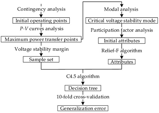
Figure 1.
Framework of proposed method.
3. Case Study
The proposed online VSM assessment method was verified using actual data obtained from a provincial power grid in China. Figure 2 displays the single-line diagram.
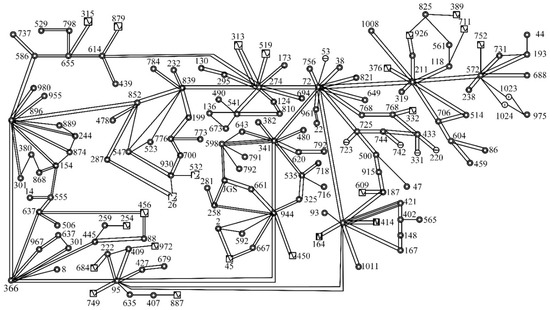
Figure 2.
Single-line diagram of the provincial power grid.
3.1. Establish the Sample Set for DT
In order to obtain different operating conditions, contingency analysis was performed on each generator, part of transmission lines, and transformer. As described in Section 2.1, P-V curve analysis was conducted for each operating condition. The maximum power transfer points can be generated by increasing system loads in 10 MW steps from the initial operating points. According to (1), the operating points in the different three system states are obtained. The points in the emergency state are regarded as emergency samples because in practice operators need to prevent the system from operating in this region. The operating points in the normal and alert states are used as normal and alert samples, respectively. To emphasize the emergency state and acquire sufficient samples for the DT, 15 samples were selected from each VSM interval in this study. The sample set included 21,960 samples in total.
3.2. Select Attributes for DT
3.2.1. Initial Selection of Attributes
As described in Section 2.2, the critical voltage stability modes are determined by modal analysis. The corresponding smallest eigenvalue of the practical system was 0.053111. In order to determine the main factors for the critical mode, PF analysis was performed. Figure 3 shows the bus PF analysis results, which are listed in descending order. The 64th factor is chosen as the threshold value based on the order of magnitudes of differences between adjacent buses. Hence, the buses whose PFs rank in the top 64 are regarded as key buses. The bus PF analysis results are shown in Table 2.
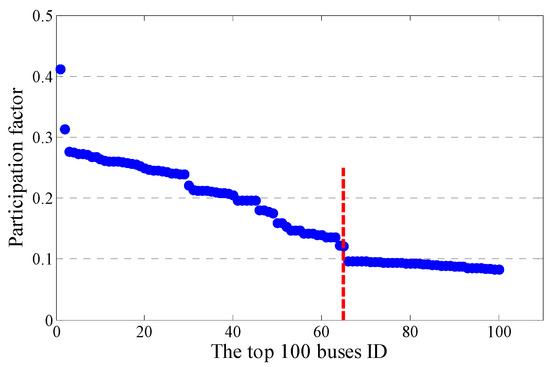
Figure 3.
Participation factors (PFs) of the top 100 buses.
Table 2.
Bus PF analysis results.
A total of 21 Key branches and 12 key generators were determined using similar methods. The branch and generator PF analysis results are given in Table 3 and Table 4, respectively. There are 161 initial attributes in total.
Table 3.
Branch PF analysis results.
Table 4.
Generator PF analysis results.
3.2.2. Determination of Attributes Set
As described in Section 2.2, 161 initial attributes were further filtered using the Relief-F algorithm. According to (7), the weight values of these initial attributes were computed. Figure 4 shows the results in descending order.
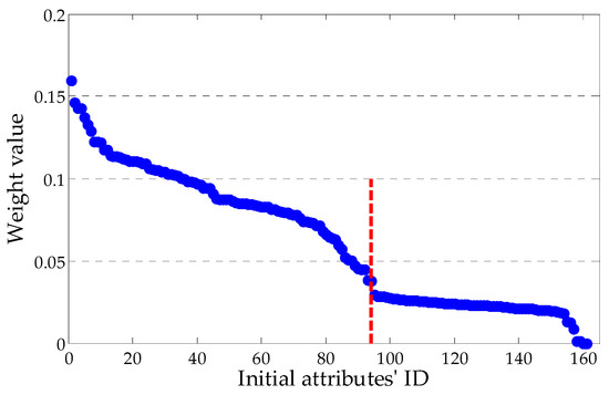
Figure 4.
Weight value associated with initial attributes.
As shown in Figure 4, the first 94 attributes were selected to construct the attribute set of the DT.
3.3. Apply C4.5 Algorithm to Build DT
The DT can be constructed based on the generated sample set and the pre-selected 94 attributes using the C4.5 algorithm. The partial DT is shown in Figure 5.
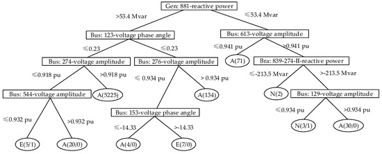
Figure 5.
Partial decision tree (DT).
In Figure 5, the first and second number in the leaf nodes indicate the total number of samples and the number of mis-classified samples, respectively. Based on all paths of the constructed DT, system operators can extract a series of VSM assessment rules. For instance, if the reactive power of generator 881 is less than or equal to 53.4 Mvar and the voltage amplitude of Bus 613 is less than or equal to 0.941 pu, the system enters the alert state. According to this rule, the system states corresponding to these 71 samples are assessed as the alert state and all are classified correctly. System operators can use these guidelines based on phasor measurement unit (PMU) data to assess the system voltage stability status.
All of the 21,960 samples were classified to evaluate the DT’s performance, which was executed on an Intel Core i7 2.5-GHz CPU with 4 GB of RAM. The generalization error was 97.3953%. The performance of the DT can be visualized in Table 5.
Table 5.
Confusion matrix of the DT.
represents the number of samples that were classified from class i to class j. For example, , which equals to 138, is the number of samples that were mis-classified from class A to class N. The total number of correct classifications made by the DT was and the total number of incorrect classifications was . In practical system operation, system operators pay more attention to the classification results of samples from class E (emergency state). In this confusion matrix, among the 7320 actual samples of class E, the DT misclassified 1 for class N and 130 for class A.
Table 6 shows case study results of the DT constructed by the C4.5 algorithm with different attribute sets.
Table 6.
The performance of the C4.5 algorithm with different attribute sets.
The modeling time of the DT constructed with 161 attributes was 13.56 s, while the modeling time of the DT constructed with 94 selected attributes was 8.45 s. This implies that the application of the Relief-F algorithm can significantly shorten the modeling time, and therefore improve the classification efficiency of the DT. The classification accuracy of the DT constructed with 161 attributes was 96.28%, while the classification accuracy of the DT constructed with 94 selected attributes was 97.40%. This implies that the application of all attributes does not guarantee a better classification accuracy. The Relief-F algorithm is an effective method to improve the performance of the DT.
Table 7 compares the performance with different DT algorithms.
Table 7.
The performance between the C4.5 and classification and regression tree (CART) algorithms.
The modeling time of the C4.5 algorithm was 8.45 s, while the modeling time of the CART algorithm was 30.34 s. Compared with the CART algorithm, the efficiency of the C4.5 algorithm was increased by about three times. The classification accuracy of the C4.5 algorithm was 4 percentage points higher than that of the CART algorithm. Hence, the C4.5 algorithm is more suitable for handling continuous attributes in VSM assessment.
Table 8 shows the classification accuracy and modeling time of the proposed method (NEW), and the ANN, SVM, and NB methods. All methods used the same sample set and the same attribute set.
Table 8.
The performance of different methods.
It is clear that the proposed method performs better than the other methods. System operators can use the operating guidelines extracted from the proposed method to monitor and assess the system state based on PMU data. Once the power system falls into the alert or emergency states, operators have enough time to enact corresponding control strategies and actions to ensure the stability of the power system.
4. Conclusions
This paper proposes constructing a DT using the C4.5 algorithm to extract operating guidelines for power system operators, and has two innovations. First, PF analysis was performed to initially select attributes based on the attributes’ physical meaning. The Relief-F algorithm was then used to further select key attributes based on the attributes’ classification ability. Second, the C4.5 algorithm was applied for constructing the DT because most of the attributes in VSM assessment are continuous variables.
Operational planners can use the DT to extract operating guidelines from a large amount of offline study data. The DT can be used to help find new knowledge and insights from offline voltage stability analysis. System operators can use the DT to quickly assess the system voltage margin based on measurement data. Operational planners can use the DT to develop effective control strategies and actions. A case study using provincial power system data indicates that the proposed VSM assessment method not only guarantees classification accuracy to meet practical system operation needs, but also handles a large amount of data within online operation requirements.
Author Contributions
X.M. and P.Z. conceptualized the paper and designed the methods; X.M. worked on the simulation results and was involved in the paper writing. D.Z. was involved in the paper modification. All authors have read and agreed to the published version of the manuscript.
Funding
This research was supported by the Beijing Jiaotong University Foundation (Grant No. KERC18001532).
Acknowledgments
The authors would like to thank the Beijing Jiaotong University Power System Laboratory.
Conflicts of Interest
The authors declare no conflict of interest.
References
- Kundur, P. Power System Stability and Control; McGraw-Hill: New York, NY, USA, 1994. [Google Scholar]
- Taylor, C.W. Power System Voltage Stability; McGraw-Hill: New York, NY, USA, 1994. [Google Scholar]
- Kundur, P.; Paserba, J.; Ajjarapu, V.; Andersson, G.; Bose, A.; Canizares, C.; Hatziargyriou, N.D.; Hill, D.J.; Stankovic, A.M.; Taylor, C.; et al. Definition and classification of power system stability. IEEE Trans. Power Syst. 2004, 19, 1387–1401. [Google Scholar]
- Van Cutsem, T.; Vournas, C. Voltage Stability of Electric Power Systems; Springer Science & Business Media: Berlin, Germany, 2007. [Google Scholar]
- Zhou, D.; Annakkage, U.D.; Rajapakse, A.D. Online monitoring of voltage stability margin using an artificial neural network. IEEE Trans. Power Syst. 2010, 25, 1566–1574. [Google Scholar] [CrossRef]
- Kalyani, S.; Swarup, K.S. Classification and assessment of power system security using multiclass SVM. IEEE Trans. Syst. Man Cybern. C 2010, 41, 753–758. [Google Scholar] [CrossRef]
- Sode-Yome, A.; Lee, K.Y. Neural network based loading margin approximation for static voltage stability in power systems. In Proceedings of the IEEE PES General Meeting, Providence, RI, USA, 25–29 July 2010; pp. 1–6. [Google Scholar]
- Innah, H.; Hiyama, T. A real time PMU data and neural network approach to analyze voltage stability. In Proceedings of the 2011 International Conference on Advanced Power System Automation and Protection, Beijing, China, 16–20 October 2011; pp. 1263–1267. [Google Scholar]
- Zhang, R.; Xu, Y.; Dong, Z.Y.; Zhang, P.; Wong, K.P. Voltage stability margin prediction by ensemble based extreme learning machine. In Proceedings of the 2013 IEEE Power & Energy Society General Meeting, Vancouver, BC, Canada, 22–26 July 2013; pp. 1–5. [Google Scholar]
- Sajan, K.S.; Tyagi, B.; Kumar, V. Genetic algorithm based artificial neural network model for voltage stability monitoring. In Proceedings of the 2014 Eighteenth National Power Systems Conference, Guwahati, India, 18–20 December 2014; pp. 1–5. [Google Scholar]
- AbAziz, N.F.; Rahman, T.K.A.; Zakaria, Z. Voltage stability prediction by using artificial immune least square support vector machines (AILSVM). In Proceedings of the 2014 IEEE 8th International Power Engineering and Optimization Conference, Langkawi, Malaysia, 24–25 March 2014; pp. 613–618. [Google Scholar]
- Duraipandy, P.; Devaraj, D. On-line voltage stability assessment using least squares support vector machine with reduced input features. In Proceedings of the 2014 International Conference on Control, Instrumentation, Communication and Computational Technologies, Kanyakumari, India, 10–11 July 2014; pp. 1070–1074. [Google Scholar]
- Sajan, K.S.; Kumar, V.; Tyagi, B. ICA based Artificial Neural Network model for voltage stability monitoring. In Proceedings of the TENCON 2015-2015 IEEE Region 10 Conference, Macao, China, 1–4 November 2015; pp. 1–3. [Google Scholar]
- Xu, Y.; Zhang, R.; Zhao, J.; Dong, Z.Y.; Wang, D.; Yang, H.; Wong, K.P. Assessing short-term voltage stability of electric power systems by a hierarchical intelligent system. IEEE Trans. Neural Netw. Learn. Syst. 2015, 27, 1686–1696. [Google Scholar] [CrossRef] [PubMed]
- Vakili, S.; Zhao, Q.; Tong, L. Bayesian quickest short-term voltage instability detection in power systems. In Proceedings of the 2015 54th IEEE Conference on Decision and Control, Osaka, Japan, 15–18 December 2015; pp. 7214–7219. [Google Scholar]
- Sajan, K.S.; Kumar, V.; Tyagi, B. Genetic algorithm based support vector machine for on-line voltage stability monitoring. Int. J. Electr. Power Energy Syst. 2015, 73, 200–208. [Google Scholar] [CrossRef]
- Subramani, C.; Jimoh, A.A.; Kiran, S.H. Artificial neural network based voltage stability analysis in power system. In Proceedings of the 2016 International Conference on Circuit, Power and Computing Technologies, Nagercoil, India, 18–19 March 2016; pp. 1–4. [Google Scholar]
- Shukla, A.; Verma, K.; Kumar, R. Online voltage stability monitoring of distribution system using optimized support vector machine. In Proceedings of the 2016 IEEE 6th International Conference on Power Systems, New Delhi, India, 4–6 March 2016; pp. 1–6. [Google Scholar]
- Malbasa, V.; Zheng, C.; Chen, P.C.; Popovic, T.; Kezunovic, M. Voltage stability prediction using active machine learning. IEEE Trans. Smart Grid 2017, 8, 3117–3124. [Google Scholar] [CrossRef]
- Ashraf, S.M.; Gupta, A.; Choudhary, D.K.; Chakrabarti, S. Voltage stability monitoring of power systems using reduced network and artificial neural network. Int. J. Electr. Power Energy Syst. 2017, 87, 43–51. [Google Scholar] [CrossRef]
- Wang, Y.; Pulgar-Painemal, H.; Sun, K. Online analysis of voltage security in a microgrid using convolutional neural networks. In Proceedings of the 2017 IEEE Power & Energy Society General Meeting, Chicago, IL, USA, 16–20 July 2017; pp. 1–5. [Google Scholar]
- Li, S.; Ajjarapu, V.; Djukanovic, M. Adaptive online monitoring of voltage stability margin via local regression. IEEE Trans. Power Syst. 2018, 33, 701–713. [Google Scholar] [CrossRef]
- Amroune, M.; Bouktir, T.; Musirin, I. Power system voltage stability assessment using a hybrid approach combining dragonfly optimization algorithm and support vector regression. Arab. J. Sci. Eng. 2018, 43, 3023–3036. [Google Scholar] [CrossRef]
- Yang, H.; Zhang, W.; Chen, J.; Wang, L. PMU-based voltage stability prediction using least square support vector machine with online learning. Electr. Power Syst. Res. 2018, 160, 234–242. [Google Scholar] [CrossRef]
- Maaji, S.S.; Cosma, G.; Taherkhani, A.; Alani, A.A.; McGinnity, T.M. On-line voltage stability monitoring using an Ensemble AdaBoost classifier. In Proceedings of the 2018 4th International Conference on Information Management (ICIM), Oxford, UK, 25–27 May 2018; pp. 253–259. [Google Scholar]
- Shakerighadi, B.; Aminifar, F.; Afsharnia, S. Power systems wide-area voltage stability assessment considering dissimilar load variations and credible contingencies. J. Mod. Power Syst. Clean Energy 2019, 7, 78–87. [Google Scholar] [CrossRef]
- Hagmar, H.; Carlsot, O.; Eriksson, R. On-Line voltage instability prediction using an artificial neural network. In Proceedings of the 2019 IEEE Milan PowerTech, Milan, Italy, 23–27 June 2019; pp. 1–6. [Google Scholar]
- Cai, H.; Ma, H.; Hill, D. A data-based learning and control method for long-term voltage stability. IEEE Trans. Power Syst. 2020, 1, 99. [Google Scholar] [CrossRef]
- Alimi, O.A.; Ouahada, K.; Abu-Mahfouz, A.M. A review of machine learning approaches to power system security and stability. IEEE Access 2020, 8, 113512–113531. [Google Scholar] [CrossRef]
- Han, J.; Pei, J.; Kamber, M. Data Mining: Concepts and Techniques; Elsevier: Amsterdam, The Netherlands, 2011. [Google Scholar]
- Zaki, M.J.; Meira, W., Jr.; Meira, W. Data Mining and Analysis: Fundamental Concepts and Algorithms; Cambridge University Press: Cambridge, UK, 2014. [Google Scholar]
- Sun, K.; Likhate, S.; Vittal, V.; Kolluri, S.; Mandal, S. An online dynamic security assessment scheme using phasor measurements and decision trees. IEEE Trans. Power Syst. 2007, 22, 1935–1943. [Google Scholar] [CrossRef]
- Diao, R.; Sun, K.; Vittal, V.; O’Keefe, R.; Richardson, M.; Bhatt, N.P.; Stradford, D.; Sarawgi, S.K. Decision tree-based online voltage security assessment using PMU measurements. IEEE Trans. Power Syst. 2009, 24, 832–839. [Google Scholar] [CrossRef]
- Vittal, V. Application of phasor measurements for dynamic security assessment using decision trees. In Proceedings of the 2012 IEEE Power and Energy Society General Meeting, San Diego, CA, USA, 22–26 July 2012; pp. 1–3. [Google Scholar]
- Zheng, C.; Malbasa, V.; Kezunovic, M. A fast stability assessment scheme based on classification and regression tree. In Proceedings of the 2012 IEEE International Conference on Power System Technology, Auckland, New Zealand, 23–26 October 2012; pp. 1–6. [Google Scholar]
- Teng, Y.; Huo, T.; Liu, B.; Tang, J.; Zhang, Z. Regional voltage stability prediction based on decision tree algorithm. In Proceedings of the 2015 International Conference on Intelligent Transportation, Big Data and Smart City, Halong Bay, Vietnam, 19–20 December 2015; pp. 588–591. [Google Scholar]
- Tan, P.N. Introduction to Data Mining; Pearson Education: New York, NY, USA, 2018. [Google Scholar]
- Khoshkhoo, H.; Shahrtash, S.M. On-line dynamic voltage instability prediction based on decision tree supported by a wide-area measurement system. IET Gener. Transm. Distrib. 2012, 6, 1143–1152. [Google Scholar] [CrossRef]
- Beiraghi, M.; Ranjbar, A.M. Online voltage security assessment based on wide-area measurements. IEEE Trans. Power Deliv. 2013, 28, 989–997. [Google Scholar] [CrossRef]
- Suprême, H.; Heniche-Oussédik, A.; Kamwa, I.; Dessaint, L.A. A novel approach for instability detection based on wide-area measurements and new predictors. In Proceedings of the 2016 IEEE Canadian Conference on Electrical and Computer Engineering, Vancouver, BC, Canada, 15–18 May 2016; pp. 1–6. [Google Scholar]
- Nie, Z.; Yang, D.; Centeno, V.; Jones, K.D. A PMU-based voltage security assessment framework using Hoeffding-tree-based learning. In Proceedings of the 19th International Conference on Intelligent System Application to Power Systems, San Antonio, TX, USA, 17–20 September 2017; pp. 1–6. [Google Scholar]
- Su, H.Y.; Liu, T.Y. Enhanced-online-random-forest model for static voltage stability assessment using wide area measurements. IEEE Trans. Power Syst. 2018, 33, 6696–6704. [Google Scholar] [CrossRef]
- Meng, X.F.; Zhang, P.; Xu, Y.; Xie, H. Construction of decision tree based on C4.5 algorithm for online voltage stability assessment. Int. J. Electr. Power Energy Syst. 2020, 118. [Google Scholar] [CrossRef]
- Witten, I.H.; Frank, E. Data Mining: Practical Machine Learning Tools and Techniques; Morgan Kaufmann: San Francisco, CA, USA, 2005. [Google Scholar]
- Dash, M.; Liu, H. Feature selection for classification. Intell. Data Anal. 1997, 1, 131–156. [Google Scholar] [CrossRef]
- Robnik-Šikonja, M.; Kononenko, I. Theoretical and empirical analysis of ReliefF and RReliefF. Mach. Learn. 2003, 53, 23–69. [Google Scholar] [CrossRef]
- Sun, Y. Iterative RELIEF for feature weighting: Algorithms, theories, and applications. IEEE Trans. Pattern Anal. 2007, 29, 1035–1051. [Google Scholar] [CrossRef] [PubMed]
- Tang, J.; Alelyani, S.; Liu, H. Feature selection for classification: A review. Data Classif. Algorithms Appl. 2014, 37. [Google Scholar] [CrossRef]
- Rong, M.; Gong, D.; Gao, X. Feature selection and its use in big data: Challenges, methods, and trends. IEEE Access 2019, 7, 19709–19725. [Google Scholar] [CrossRef]
- Quinlan, J.R. C4.5: Programs for Machine Learning; Elsevier: Amsterdam, The Netherlands, 2014. [Google Scholar]


© 2020 by the authors. Licensee MDPI, Basel, Switzerland. This article is an open access article distributed under the terms and conditions of the Creative Commons Attribution (CC BY) license (http://creativecommons.org/licenses/by/4.0/).