Decarbonization of Australia’s Energy System: Integrated Modeling of the Transformation of Electricity, Transportation, and Industrial Sectors

Abstract

To achieve the Paris Agreement’s long-term temperature goal, current energy systems must be transformed. Australia represents an interesting case for energy system transformation modeling: with a power system dominated by fossil fuels and, specifically, with a heavy coal component, there is at the same time a vast potential for expansion and use of renewables. We used the multi-sectoral Australian Energy Modeling System (AUSeMOSYS) to perform an integrated analysis of implications for the electricity, transport, and selected industry sectors to the mid-century. The state-level resolution allows representation of regional discrepancies in renewable supply and the quantification of inter-regional grid extensions necessary for the physical integration of variable renewables. We investigated the impacts of different CO₂ budgets and selected key factors on energy system transformation. Results indicate that coal-fired generation has to be phased out completely by 2030 and a fully renewable electricity supply achieved in the 2030s according to the cost-optimal pathway implied by the 1.5 °C Paris Agreement-compatible carbon budget. Wind and solar PV can play a dominant role in decarbonizing Australia’s energy system with continuous growth of demand due to the strong electrification of linked energy sectors.

1. Introduction

The commitment by the world community to meet the Paris Agreement’s (PA) [1] long-term temperature goal (LTTG) of 1.5 °C has led to an increasing awareness of the urgency for extensive energy system transformation to achieve rapid and dramatic reduction of global greenhouse gas (GHG) emissions. Rising penetration of renewable energy sources across increasingly coupled and electrified energy sectors plays a crucial role in the global response to the threat of climate change [2]. However, integration of variable renewable energy sources (VRES) raises the concerns of a flexibility gap in the system to ensure the security of supply with increasing shares of VRES. Sector coupling is thus emerging as a crucial topic to eliminate emissions from distributed sources, such as in the transport sector, while also increasing the flexibility of end-use sectors and thereby raising the system’s capability to integrate high shares of VRES across all energy sectors [3].

Australia represents an interesting case for energy system transformation analysis. While it currently has a power system dominated by fossil fuels and, specifically, coal, the country is also endowed with a vast potential for expansion and use of renewable energy. Geographically, the country is divided into seven states and territories (New South Wales (NSW), Queensland (QLD), South Australia (SA), Tasmania (TAS), Vitoria (VIC), Western Australia (WA), and Northern Territory (NT), two of which (WA and NT) have power systems isolated from the rest of the country’s which is interconnected through the National Electricity Market (NEM). Regions currently have widely differing characteristic energy mixes and resources, ranging from high reliance on brown coal (VIC), black coal (NSW, QLD) and natural gas (WA, NT) to states that have already moved toward renewable energy-dominant systems (SA, TAS). Renewable power systems across Australia are experiencing rapid growth, particularly in solar photovoltaics and to a lesser extent with wind power and battery storage.

Several studies have focused specifically on the modeling and scenario analysis of the Australian energy system and assessing its CO₂ emissions footprint by applying heterogenous methodologies. The studies incorporate different regional scopes, taking into account Australia as one aggregated region or looking into the sub-national level. For instance, the study in Reference [4] investigates how Australia’s energy portfolio contributes to CO₂ emissions and environmental degradation through modern econometric methods and applying empirical analysis. Reference [5] adopted a system dynamic approach to construct an integrated model for analyzing the behavior of the Australian energy sector. However, the methodology is limited in its ability to simulate the dynamics of sectoral transformation pathways over time. The applied methodology also cannot be used to investigate the implications of cross-regional power transmission as a cost-effective measure for the integration of VRES.

References [6,7,8] project long-term development pathways for the energy system of Australia using the Australian TIMES model for national energy technology uptake. References [6,7] further combine the quantitative analyses with the Victoria University Regional Model (VURM) for national energy demand projections and the Global and Local Learning Model (GALLM) for technology learning at the global scale. In Reference [6], the greatest emissions reduction comes from electricity and transport sectors in 2050 under the scenarios analyzed. Reference [7] presents three scenarios of Slow Decline, Thriving Australia, and Green and Growth for the energy system transformation of Australia based on the ambition level of decarbonization goals and global cooperation to achieve them. Reference [8] presents decarbonization scenarios for various energy sectors and sub-sectors of Australia using a cost-optimization approach. While the scenarios in Reference [6] rely on the application of carbon capture and storage (CCS) in combination with dispatchable gas-based generation to decarbonize the electricity sector, the scenarios in References [7,8] depend heavily on carbon sequestration from carbon forestry to achieve overall net zero emissions. In reality, carbon forestry provides only a short-term fix for emissions abatement and may not be a reliable option in the context of Australia where the forests are vulnerable to heatwaves, droughts, and bushfires—many of which are being made worse due to the fact of climate change [8].

In Reference [9], a discrete numerical computational approach was used to model the CO₂ emissions from Australia’s electricity sector, transitioning from the fossil fuel-based system of today towards a renewable-based supply. The study investigated ambitious renewable scenarios, considering a transformation to predominantly renewable electricity, where in some cases up to 98% of electricity is to be generated by renewable sources by no later than 2030. Reference [10] also focuses on the role of electrical energy storage to enable the renewable energy transition in Australia. Reference [11] combines retrospective and exploratory scenarios using the Long Range Energy Alternatives Planning (LEAP) system and its integrated Open Source Energy Modelling System (OSeMOSYS) to explore the least-cost electricity generation expansion options for Australia. The study identifies carbon tax policies as being more cost-effective as compared to emission reduction policies. However, the study lacks sensitivity tests with different projections of fuel prices and costs of energy technologies. The modelling exercises conducted in References [9,10,11] do not consider the role of the sector-coupling options in adding system flexibility to reduce the need for electricity storage and to reduce the overall GHG emissions from the energy system.

Reference [12] investigated the transition of the Australian energy system towards a renewable-based supply until 2050, applying a bottom-up integrated energy balance simulation-based model with various parameters and future projections specified exogenously as input, including the market share of each technology with respect to total heat or electricity production. Therefore, the applied methodology is not capable of providing insights on cost-optimal endogenously dynamic sectoral transformation pathways. Furthermore, the aggregated representation of the Australian energy system does not allow analyzing the regional implications as well as required extension of the transmission grid for highly renewable scenarios. The low-carbon transformation of the Australian National Electricity Market (NEM) alone has also been investigated [13,14,15,16,17,18]. Reference [13] presents an hourly energy balance of the Australian NEM interconnected electricity market in a 100% renewable energy scenario, while Reference [14] performed a simulation of low-carbon electricity supply for Australia by applying a spatial optimization process for identifying suitable generator locations. Reference [15] identifies integration of large quantities of wind as the single most important factor towards cost-optimal solution for the 100% renewable energy portfolios in the NEM. While this study focused only on existing economically operating technologies, the implications of technology and cost breakthroughs for novel storage and renewable generation technologies are out of the scope of the study that could substantially affect the assessment of energy system transformation. References [16,17,18] applied least-cost modeling to determine the cost-optimal combination of generation and storage investments to satisfy the given exogenous electricity demand of the NEM interconnected supply area over a time horizon until 2040 or 2050. References [19,20,21] simulated partial and full renewable supply scenarios for the South West Interconnected System (SWIS). The latter studies concluded that a battery-based system operating at almost 100% renewable energy would be no more expensive than a conventional fossil system. Reference [22] provides an overview of various scenario analyses of power system transformations of Australia (excluding the Northern Territory) to 2050 and its implications. The roadmap scenario in this study achieved net zero emissions by 2050; this is consolidated by the orchestration of distributed energy resources. The regional scope of these studies, focusing on a subset of states and territories, limits the insights that could be obtained by a full Australian energy system model with a detailed regional resolution, covering all states and territories.

The potential of regional interconnection between Australia and other South East Asian countries in the region have been explored in References [23,24,25]. Reference [23] investigated the role of a submarine high-voltage direct-current (HVDC) link connecting Indonesia’s Java–Bali power grid to the NEM grid through the Northern Territory. The study concluded that despite the expensiveness of long HVDC lines, it offers a cost-effective measure to meet Indonesia’s growing electricity demand by utilizing Australia’s abundant renewable energy sources. This further allows to benefit from the smoothening effects of the output power through the distribution of VRES across a large interconnected area. Reference [24] depicts a cost-optimal 100% renewable energy-based system for Southeast Asia and the Pacific Rim region for the year 2030 on an hourly resolution. Although the study concludes that an optimal electricity mix in Australia would be dominated by photovoltaic (PV) power closely followed by wind, it does not provide a state-wise resolution of electricity mix for the country, and it also does not take into account the potential additional electricity demand from the uptake of electric vehicles in the future. Furthermore, the study provides only the medium-term projections of electricity mix until 2030 without investigating the sector through the long-term horizon.

Most of the studies reviewed provide decarbonization pathways either for the NEM region or the SWIS in Australia. Some studies model the energy system for Australia in an aggregate level. Other studies offer renewable energy roadmaps with regional interconnection between energy systems of Australia and South East Asian countries. However, those studies do not incorporate a detailed state-wise resolution model of the Australian energy system in an integrated manner. Thus, the regional implications of the low carbon transformation pathways for different Australian states is missing in the former studies. Furthermore, linkages between previously independent energy sectors will become increasingly important in the near future. Besides cross-border integration, cross-sectoral integration (i.e., linking the power and transportation as well as industry sectors through direct use of renewable electricity or indirect electrification through use of renewably produced hydrogen and synthetic fuels) is a crucial and ongoing research topic [3].

To bridge the gaps, we propose a multi-sectoral, multi-regional approach for modeling the Australia’s energy system. We analyzed various potential decarbonization pathways of Australia’s energy system, detaching from a fossil fuel-based system of today towards a carbon-neutral energy system. Applying an integrated energy system modeling approach enables us to analyze the implications for different energy sectors beyond the power sector only. To our knowledge at present this is the first time a model has been implemented to provide cost-optimal technology mix solutions for Australia with state-level resolution and a detailed representation of different flexibility options such as regional interconnection and coupling between sectors like cement, steel, electricity, and transport at the same time. We have developed the multi-sectoral Australian Energy Modeling System (AUSeMOSYS) based on the open-source energy modeling system (OSeMOSYS) framework [26]. We applied AUSeMOSYS to investigate cost-optimal transformation pathways towards a zero-carbon Australian energy system by mid-century. The model was calibrated to recent past trends in energy generation, including the recent and near-future rapid uptake of renewables in different regions, whether by policy decision or autonomous development. Beyond the power sector, AUSeMOSYS also provides scenario pathways for the uptake of electric vehicles and hydrogen-powered transport, coupled to the power sector with a timeline through 2050. To investigate the full extent of renewable energy expansion given Australia’s recognized large renewable energy resource potential, we linked selected industrial sectors to the power system, e.g., steel production, where use of electric generation can further decarbonize Australia’s economy either directly or via hydrogen production and use. A detailed, state-level resolution of the model allows for the representation of regional characteristics in renewable supply and energy demand and enables us to quantify transmission grid extensions required for the large-scale integration of VRES. The model is thus able to mimic complex interactions of system components within a multi-regional, multi-sectoral interconnected energy supply system under various scenarios that impose boundary conditions on the system. We further investigated sensitivities to key parameters that can affect the uptake and use of renewable energy.

The paper proceeds as follows: Section 2 elaborates on the methodology and provides a comprehensive overview of key assumptions and input data used for modeling the Australian energy system. Furthermore, the characterization and limitations of the applied model are presented in this section. Section 3.1 describes the scenario framework applied in this study. The model results are presented and discussed in Section 3.2. Section 4 discusses the main findings and draws conclusions.

2. Methodology

Energy system transformation pathways can be investigated using a continuous spectrum of models ranging from “top-down” models focused on the stylized representation of the broader economy and a simplified technical representation of the energy sector, to “bottom-up” models that tend to isolate the energy system but with greater technological resolution [27,28,29,30]. With climate change mitigation as a driving factor behind low-carbon energy policies, either modeling approach uses boundary conditions set by carbon budgets or costs to look for optimal solution pathways for a given goal. Prominent among modeling efforts relevant for evaluating global pathways compatible with the Paris Agreement are integrated assessment models assessed by the Intergovernmental Panel on Climate Change (IPCC) [2] which include a strong energy system modelling component.

Energy system optimization models involve an elaborated representation of interdependencies among various energy carriers, conversion technologies as well as transmission and storage systems as depicted by the Reference Energy System, thus allowing the assessment of various technological pathways and how a rich array of technologies can interact to effect systemic change over time. Typically, such models optimize overall system costs over the modeling time period subject to various user-defined technological and environmental constraints but do not couple into a model of the broader economy as a whole. The detailed technological nature of energy system optimization models allows the simulation of a wide variety of both micro measures (e.g., technology portfolios or targeted subsidies to groups of technologies) and broader policy targets (e.g., a general carbon tax or permit trading systems), and such models are capable of analyzing various regional and national policies due to the fact of their level of technical and geographical detail. Limiting the scope to modeling the energy sector allows incorporating a high level of detail not only in terms of energy sectors and technologies but also with respect to geographical or temporal resolution. This allows moving from global and regional modeling and projections and to concentrating on the specifics of individual countries and regions within countries. This is of particular relevance when assessing the energy system integration impacts of VRES due to the fact of their temporal fluctuations and geographical dispersion.

In this work, we adapted OSeMOSYS, a full-fledged optimization framework for long-range energy system and GHG pathways, to create a new model named AUSeMOSYS, a multi-regional, multi-sectoral energy system cost-optimization model based on the linear programming optimization method. Although sharing a broad range of characteristics with The Integrated MARKAL Energy Flow Optimization Model (EFOM) (TIMES) [31], the key advantages of OSeMOSYS over other long-established energy system models is being open source and having a less significant learning curve and time commitment needed to build and operate [26].

The model consists of 7 regions: NSW (Australian Capital Territory (ACT) is covered in NSW), QLD, SA, TAS), VIC, WA, and NT. The state-level resolution of the model allows for the representation of regional discrepancies in terms of renewable supply and demand as well as sub-national/state-level imposed energy and climate policies and targets. New investments in power generation, storage, and inter-regional power transmission are optimized by considering the development of demand over time while the electricity demand for electrification of selected end-use sectors, particularly relevant under stringent mitigation scenarios, is treated endogenously. The temporal resolution is limited according to the accessible computation power and due to the long calculation time. The current version of the model covers a time horizon until 2050 with annual time steps until 2025 followed by 5 year time steps through 2050. The sub-annual resolution of the model is defined by eight time slices in this version of the model. For this model specification, we chose to use four seasons (i.e., summer, winter, spring, autumn), one day type, and two daily time brackets (i.e., day, night).

2.1. Model Formulation

We used the current version of OSeMOSYS originally coded in GNU MathProg while incorporating model enhancements introduced in previous studies [32,33] as well as new additions considered most relevant for addressing the questions of the present study.

The objective function minimizes the net present value of total energy system costs and is given in Equation (1).

minimize z = Σ_r,y (Σ_t (dic_r,t,y + doc_r,t,y + … + dec_r,t,y + drc_r,t,y − dsv_r,t,y) + ⋯ Σ_f,rr dntcc_f,r,rr,y + Σ_f datc_f,r,y +Σ_s tdsc_r,s,y)

(1)

Total system costs are composed of the sum of total discounted investment (dic_r,t,y), fixed and variable operation costs (doc_r,t,y), emission costs (dec_r,t,y), annual production change costs (drc_r,t,y) minus the salvage costs (dsv_r,t,y) for each region (r), technology (t) and year (y) in the model. Furthermore, the total discounted new trade capacity costs (dntcc_f,r,rr,y) as well as annual trade costs of importing fuels (f) in each region (datc_f,r,y) are discounted back to the first modeled year and added to the objective value. In addition, the total storage costs (tdsc_r,s,y) defined as the sum of discounted investment, fixed and variable operation costs, emission costs minus the salvage value for any storage technology is taken into account in the objective function. We assumed a global discount rate of 5% for the calculations of our model. From a macroeconomic perspective, minimization of overall costs, which corresponds to maximization of producers’ and consumers’ surplus, defines an ideal operation of the energy system through a central planner.

Minimization of overall system costs is subject to different restrictions, representing energy system characteristics. A few new additions and modifications have been made in the original version of the code. In particular, to have a better representation of inter-regional power transmission, several equations and constraints have been added. The energy transport lines are modeled as trade-based interconnections. According to Equation (2), the total capacity of each power transmission line (ttc_f,r,rr,y) is equal to the previously installed capacity (etc_f,r,rr,y), given as input, plus the newly installed capacity (ntc_f,r,rr,y) which is optimized.

ttc_f,r,rr,y = Σ_{y∈(y − yy)>0} ntc_r,rr,f,yy + etc_f,r,rr,y

(2)

Constraints Equations (3) and (4) limit the inter-regional energy flow (Imp_f,l,r,rr,y and exp_f,l,r,rr,y) at each time slice (l) of the year according to the total available transmission capacity (ttc_f,r,rr,y).

Imp_f,l,r,rr,y ≤ ttc_f,r,rr,y

(3)

exp_f,l,r,rr,y ≤ ttc_f,r,rr,y

(4)

Equation (5) represents the energy balance by taking into account the transmission losses (TLF_f,r,rr,y).

Imp_f,l,r,rr,y ≤ (1 − TLF_f,r,rr,y) × exp_f,l,r,rr,y

(5)

Further constraints limit new investments of inter-regional transmission capacities according to user-defined parameters of capacity growth rate (GRTC_r,rr,f,y) as reflected in Equation (6), and the capacity upper limit (MTTC_r,rr,f,y) as given in Equation (7). These capacity constraints are applied to avoid sudden, unrealistic increase of trade capacities over time.

ttc_f,r,rr,y ≤ (1 + GRTC_f,r,rr,y) × ttc_{f,r,rr,y − 1}

(6)

ttc_f,r,rr,y ≤ MTTC_f,r,rr,y

(7)

Dynamic activity constraints, represented in Equations (8) and (9), limit the ramp-up and ramp-down of generation from different power plant technologies (ttac_r,t,y) between the two consecutive model time steps according to the user-defined parameters of ACTRU_r,t,y and ACTRL_r,t,y.

ttac_r,t,y ≤ (1 + ACTRU_r,t,y) × ttac_{r,t,y − 1}

(8)

ttac_r,t,y ≥ (1 − ACTRL_r,t,y) × ttac_{r,t,y − 1}

(9)

Technology growth constraints are an important complementary to the model. The new capacity investments based on cost-optimization might lead to the sudden ramp up of a specific technology which achieves the cost parity with conventional technologies due to the learning effects and declining costs of renewables over time, for instance. However, this might be interpreted as unrealistic when comparing against real circumstances due to the infrastructural and institutional barriers which cannot be directly reflected in the models. The life cycles of technological innovations can be described using an S-curve trajectory which maps the initial exponential growth, increasing adoption, and final saturation of a new technology.

Equation (10) limits the growth of electric cars on the road according to the user-defined input parameter representing maximum share of electric vehicles in total road vehicle stock over time (MEVSH_r,y). Total number of electric cars on the road at each year (evca_r,y) is thus limited to the multiplication of the given maximum EV share (MEVSH_r,y) and the total number of cars on the road (trca_r,y). The input parameter (MEVSH_r,y) can be informed, for instance, by existing scenario literature on the plausible development pathways of electric vehicles for the country of interest or alternatively by assuming an S-curve trajectory towards full exploitation of potential in the long-term.

evca_r,y ≤ MEVSH_r,y × trca_r,y

(10)

The remainder of the model formulation is well described in previous studies [26,32,33,34]. Model equations as well as a list of symbols used are provided in Appendix A.

2.2. Key Assumptions and Input Data

As with all models, it is crucial to be clear about what assumptions are being made in the model and then to do sensitivity analysis on the key factors. This section provides an overview on the main input parameters to the model and elaborates on the data sources used. In addition, assumed techno-economic parameters and further input data are given in Appendix B as a complementary to the explanations provided below. The assumptions for the costs, conversion efficiency, and lifetime of various power plants, storage technologies, and electrolysis systems are based on an extensive review of a broad range of recent studies including Australian-specific data sources [18,33,34,35,36,37,38,39,40,41,42,43].

Table A2. Investment costs of power plant technologies (all costs are in US $2018/kW). Data based on References [18,33,36,39].

Technology	2015	2020	2025	2030	2035	2040	2045	2050
Coal power plant–subcritical	2115	2100	2082	2066	2049	2033	2016	2000
Coal power plant–supercritical	2327	2309	2291	2272	2254	2236	2218	2200
Lignite power plant	3592	3564	3535	3502	3473	3446	3419	3396
Oil power plant	742	750	750	750	750	750	750	750
Gas power plant (OCGT)	637	634	629	624	619	614	609	604
Gas power plant (CCGT)	913	906	900	892	885	878	870	863
PV utility 1	2178	808	586	511	448	383	359	332
PV rooftop 1	2469	784	577	503	440	378	354	328
Wind onshore	1180	1113	1021	943	912	882	870	870
Wind offshore	3320	3189	2890	2669	2583	2497	2462	2462
Biomass power plant	3017	2876	2740	2601	2481	2360	2250	2140
Geothermal power plant	5738	5455	5180	4906	4659	4412	4187	3962
Hydro power plant	2415	2415	2415	2415	2415	2415	2415	2415

¹ The high VRE scenario from the Australian-specific data source Reference [36] was used as an ambitious range of the PV utility and PV rooftop costs specific to Australia.

,

Table A3. Sensitivity case on higher investment costs assumptions for solar PV (all costs are in US $2018/kW). Data based on Reference [36].

Technology	2020	2025	2030	2035	2040	2045	2050
PV–Utility	886	651	559	498	451	406	375
PV–Rooftop	823	611	525	466	423	381	352

The central scenario from the Australian-specific data source Reference [36] was used as an ambitious range of the PV utility and PV rooftop costs specific to Australia.

,

Table A4. Operational lifetime of various power plant technologies. Data based on [18,36,37,39,46].

Technology	Lifetime (Years)
Coal power plant–subcritical	50
Coal power plant–supercritical	50
Lignite power plant	50
Oil power plant	30
Gas power plant (OCGT)	35
Gas power plant (CCGT)	35
PV utility	30
PV rooftop	30
Wind onshore	25
Wind offshore	25
Biomass power plant	30
Geothermal power plant	40
Hydro power plant	70

,

Table A5. Conversion efficiency of various power plant technologies. Data based on References [33,36,37,38,39].

Technology	Efficiency (%) 1
Coal power plant–subcritical	37%
Coal power plant–supercritical	40%
Lignite power plant	32%
Oil power plant	31%
Gas power plant (OCGT)	31%
Gas power plant (CCGT)	51%

¹ Note: As mature technologies no major efficiency improvement over time is assumed for conventional thermal power plants.

,

Table A6. Investment costs of storage systems (all costs are in US$2018). Data based on [38,39,40,92].

Technology	Parameter	Unit	2015	2020	2025	2030	2035	2040	2045	2050
PHES	Capex	$/kWhel	8	8	8	8	8	8	8	8
PHES–interface	Capex	$/kWel	713	713	713	713	713	713	713	713
PHES–Total system costs 1	Capex	$/kWel	781	781	781	781	781	781	781	781
	Opex fix	$/kWel/a	12	12	12	12	12	12	12	12
Battery storage–Battery pack	Capex	$/kWhel	204	160	100	67	60	54	47	41
Battery storage–Balance of System (BOS)	Capex	$/kWel	668	523	323	219	197	176	154	133
Battery storage–Total system costs 2	Capex	$/kWel	1484	1162	718	486	436	391	343	300
	Opex fix	$/kWel/a	37	29	18	12	11	10	9	7
Hydrogen storage–Salt caverns	Capex	$/kWhH2,LHV	0.36	0.36	0.36	0.36	0.36	0.36	0.36	0.36
	Opex fix	$/kWhH2,LHV	0.01	0.01	0.01	0.01	0.01	0.01	0.01	0.01
Hydrogen storage–Pipeline	Capex	$/kWhH2,LHV	11	11	11	11	11	11	11	11
	Opex fix	$/kWhH2,LHV	0.11	0.11	0.11	0.11	0.11	0.11	0.11	0.11

¹ Total costs of PHES calculated by assuming 8 h storage. ² Total costs of Battery storage calculated by assuming 4 h storage.

,

Table A7. Higher costs assumptions for battery storage assumed in the LME scenario and sensitivity case (all costs are in US $2018). Data based on References [38,39,40,92].

Technology	Parameter	Unit	2015	2020	2025	2030	2035	2040	2045	2050
Battery storage–Battery pack	Capex	$/kWhel	204	177	133	111	104	97	91	84
Battery storage–Balance of System (BOS)	Capex	$/kWel	668	578	435	365	342	319	296	273
Battery storage–Total system costs	Capex	$/kWel	1484	1284	968	810	760	709	658	610
	Opex fix	$/kWel/a	37	32	24	20	19	18	16	15

and

Table A8. Technical parameters of storage systems. Data based on References [38,39,40,92].

Technology	Round-Trip Efficiency (%)	Energy to Power Ratio (h)	Operational Lifetime (Years)
PHES	85%	50	50
Battery	90%	4	20
Hydrogen storage–Salt cavern	100%	84	30
Hydrogen storage–Pipeline	100%	471	30

of Appendix B further elaborate on the techno-economic parameters of different power generation and storage technologies assumed in the model.

The power system model covers various fossil fuel and renewable-based power generation technologies, all contributing to satisfy the given electricity demand. Fuel prices were mainly based on the projections for OECD Pacific region as provided in Reference [44]. The lower demand for carbon-intensive fuels in the stringent mitigation scenarios resulted in lower prices than in the reference case. This was reflected in our scenario-specific assumptions for fossil fuel price projections (cf. Appendix B,

Table A9. Fuel price projections (all costs are in US $2018/GJ). Data based on Reference [44].

Scenario	Fuel	2020	2030	2040	2050
LME	Black Coal	3.3	4.4	4.5	5.3
	Brown Coal	0.6	0.8	0.8	0.9
	Oil	12.3	21.5	24.2	35.1
	Natural Gas	10.0	10.7	10.9	11.8
	Biomass	7.5	7.5	7.5	7.5
P1.5 °C	Black Coal	3.4	3.5	3.5	3.4
	Brown Coal	0.6	0.6	0.6	0.6
	Oil	10.2	12.6	13.0	14.3
	Natural Gas	9.0	9.6	10.3	13.2
	Biomass	7.5	7.5	7.5	7.5

). The capacity of operating power plants has been determined using the Platts World Electric Power Plants Database [45]. The Platts database includes the age of the power plants and, thus, the future power plant fleet per region could be extrapolated by applying technology-specific lifetimes. In addition, the retirement of existing fossil fuel power plants as notified by their owners has been taken into account based on anticipated retirement dates provided in References [18,46]. The existing and planned pumped hydro storage capacities were further complemented based on References [18,47]. According to these sources, the proposed pumped hydro storage project Snowy 2.0 in New South Wales was assumed to be commissioned in 2025. The Battery of the Nation project in Tasmania was then assumed to be installed in 2033. Existing and committed battery storage projects were also included according to References [48,49]. The existing PV rooftop capacity and future developments were informed based on the data provided in Reference [18].

Hourly capacity factors of solar PV and wind were calculated based on the data provided by renewables.ninja from the meteorological year 2018 [50,51]. The average values were calculated for each state and included in the model. The hourly capacity factors of VRES were assumed to remain constant over the modeled time horizon. Thus, increasing output power of wind turbines due to the increasing hub height because of technology advances was not taken into account.

Total capacity of renewable power plants that can be installed in each model region and the maximum generated electricity was limited according to the available potential. A bottom-up assessment of roof-top PV potential in Australia [52] was used to limit the maximum installable capacity and output power in each model region. The study conducted in Reference [52] assumed 90% of usable residential roofs and 10% of other usable roofs were pitched at 25° and evenly distributed among all northerly orientations, with remaining roofs being flat and shading characteristics provided by GIS modeling. In addition, they assume a derating factor of 0.77 to account for electrical efficiency losses, soiling, degradation, etc. Furthermore, several data sources have been reviewed concerning the technical potential of wind and solar energy in Australia [12,44,53]. These studies assess the technological potential, derived from the theoretical potential by considering the conversion efficiency of the respective conversion technology as well as additional restrictions regarding the area that is realistically available for energy generation. The deployment of onshore wind and utility-scale solar PV in our scenarios is limited according to the potentials as given in Reference [12]. However, Australia is characterized by a huge untapped potential for solar and wind electricity generation, and it is important to note that even the conservative assumptions of the maximum potential would not represent a binding constraint to the continued growth of VRES integration.

Table A10. Maximum installable capacity and generated electricity for roof-top PV in model regions according to the available potential. Data based on Reference [52].

Technology	Region	Technical Potential (GW)	Technical Potential (TWh/Year)
Rooftop-PV	NSW	51	69
	QLD	37	54
	VIC	45	56
	TAS	4	5
	SA	17	24
	WA	23	34
	NT	1	2
	Australia South and East (NEM)	154	208
	WA and NT	24	37
	Total Australia	178	245

,

Table A11. Maximum installable capacity and generated electricity for utility scale PV and wind onshore according to the available potential. Data based on [12,44].

Technology	Region	Technical Potential (GW) Based on [44]	Technical Potential–Conservative Assumption Based on [12]
Utility-scale PV	Australia south and East (NEM)	52,003
	WA and NT	70,345
	Total Australia	122,348	24,100 (GW); 71,700 (TWh/year)
Wind onshore	Australia south and East (NEM)	10,178
	WA and NT	13,812
	Total Australia	23,990	880 (GW); 3100 (TWh/year)

and

Table A12. VRE capacity factors. Data based on References [50,51].

Region	Solar PV	Wind Onshore
NSW	20%	29%
QLD	21%	24%
VIC	18%	31%
TAS	17%	39%
SA	19%	33%
WA	18%	37%
NT	20%	37%
Average Australia South and East (NEM)	19%	31%
WA and NT	19%	37%
Total Australia	19%	37%

of Appendix B represent the VRE capacity factors as well as maximum installable capacity in each model region.

Electricity transmission was modeled on an aggregated level based on the representative nodes, assuming one node per model region. Thus, we exclusively considered the interconnections among the model regions only; so, intra-regional interconnections or line constraints were not taken into account. The existing transmission capacities among model regions were obtained from Reference [54]. For overhead transmission, high voltage alternating current (HVAC) technology is dominantly used today. However, the direct current transmission (DC) has the advantage of higher current densities, and the length-dependent losses are considerably lower than HVAC systems. We thus assumed offshore connections are made using HVDC transmission. For onshore connections, a generic transmission technology was assumed with specific investment costs of 306 US$ per km and MW (natural power) in line with the ranges assumed in the literature [13,55]. A transmission loss factor of 4% per 1000 km was assumed based on References [55,56]. Different technology options were thus not taken into account in the model as transmission lines were not modeled individually but rather as aggregated transmission corridors. The representation of an intra-regional distribution grid as well as the inclusion of different power transmission technologies requires a more detailed modeling approach than applied here.

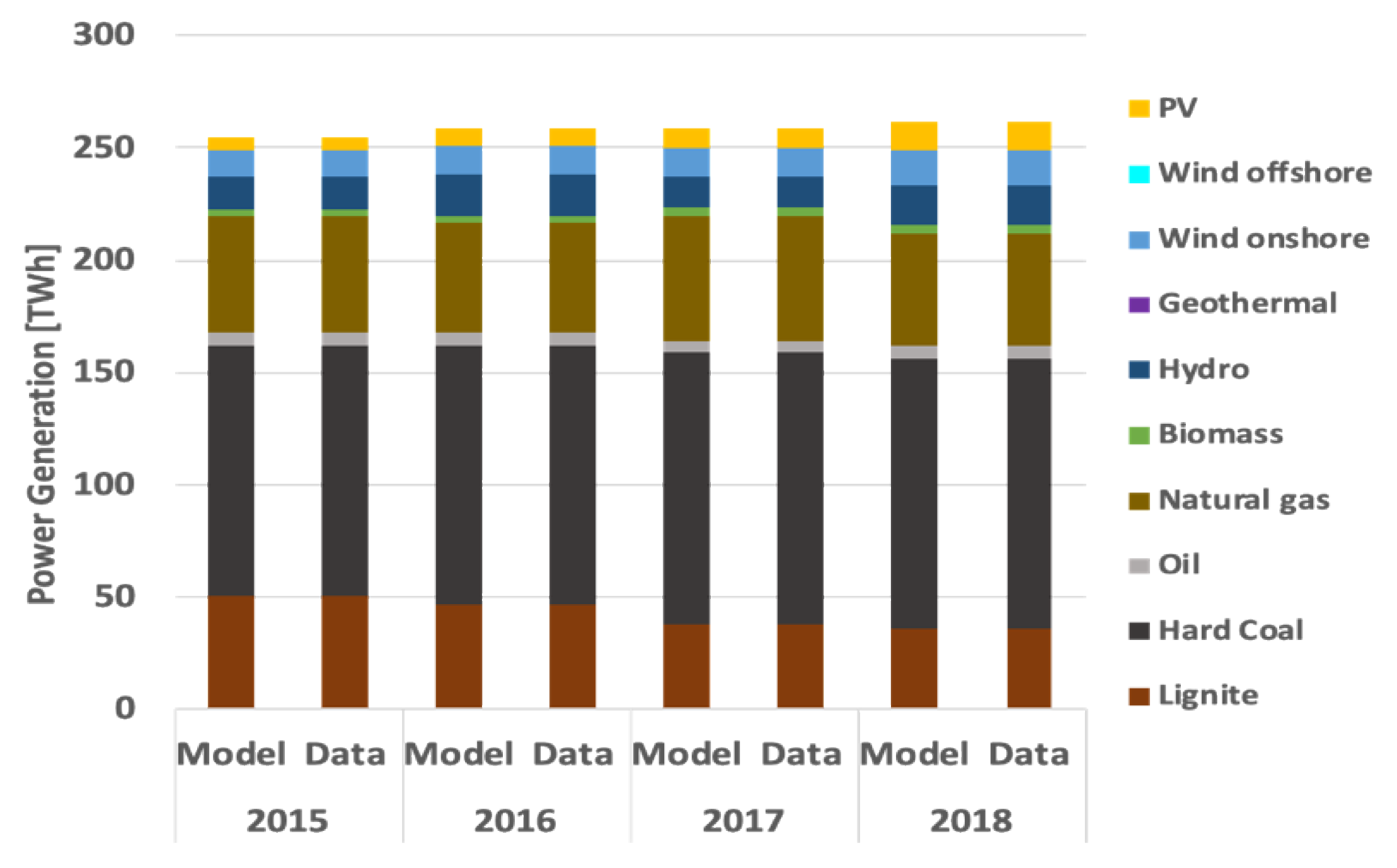
Finally, the electricity generation by different power plant technologies and fuel types over the historic period 2015–2019 from Reference [57] was applied for calibrating the model. Historic emissions from Reference [58] were used for comparison and validating the model results in terms of CO₂ emissions from electricity supply over historic period.

Beyond the power sector, an extensive data search was performed to collect data for further modeled sectors, including passenger and freight transport (in the transport sector we focused on the land-based passenger and freight transport, while aviation and shipping were not covered in this study) as well as selected industry sectors including iron, steel, and cement manufacturing industries. The modeled sectors cover a major share (72%) of Australia’s total CO₂ emissions.

The transport sector model was disaggregated into a set of different modes and vehicle technology types. The annual energy demand for each fuel was then calculated by multiplying the corresponding specific energy demand of different vehicle technology types with the given demand for energy services in terms of passenger–km and ton–km activity projections. Historical passenger and freight transport activity data as well as modal split in terms of total vehicle–kilometers travelled by different vehicle types at different states were obtained from Reference [59]. Existing stock of registered motor vehicles by state/territory over 2015–2019 was taken from References [59,60]. The current market share of battery electric vehicles (BEV) and plug-in hybrid electric vehicles (PHEVs) in Australia was taken from the historical data provided in Reference [61].

Internal combustion, battery electric, and fuel cell vehicle cost assumptions are based on the proposed ranges given by References [35,42]. Price projections for diesel and gasoline were made by applying the growth rate obtained from the reference scenario projections for crude oil from Reference [62] to historical data. Specific fuel consumption per vehicle–kilometer travelled by different vehicle types and potential efficiency improvements over time was based on a detail review of various studies including Australian-specific data sources [35,44,60,63,64,65,66]. Energy efficiency of various vehicle types and cost assumptions are given in

Table A13. Energy efficiency of various vehicle types represented in TWh/gpkm. Data based on References [35,44,60,63,64,65,66].

Technology	2015	2050
Passenger Car–ICE–Gasoline	0.78	0.65
Passenger Car–ICE–Diesel	0.69	0.57
Passenger Car–ICE–Biofuel	0.75	0.63
Passenger Car–Electric	0.18	0.15
Passenger Car–Hydrogen	0.22	0.15
Bus–Diesel	0.21	0.18
Bus–Electric	0.084	0.080
Bus–Hydrogen	0.14	0.09

and

Table A14. Internal combustion and electric vehicle cost assumptions (all costs are in 1000 US $2018). Data based on Reference [35].

Technology	Scenario	2015	2025	2030	2035	2040	2045	2050
Passenger Car–ICE–Gasoline	All	27	27	27	27	27	27	27
Passenger Car–ICE–Diesel	All	33	33	33	33	33	33	33
Passenger Car–BEV	P1.5 °C	53	30	27	27	27	27	27
Passenger Car–BEV	LME	53	40	38	36	34	32	27
Passenger Car–FCEV	P1.5 °C	53	39	34	31	30	29	27
Passenger Car–FCEV	LME	53	42	40	37	34	32	29
Bus–Diesel	All	180	180	180	180	180	180	180
Bus–BEV	P1.5 °C	290	238	214	192	192	191	180
Bus–BEV	LME	290	263	248	234	220	205	180
Bus–FCEV	P1.5 °C	242	199	192	190	180	180	180
Bus–FCEV	LME	242	221	214	208	201	195	188
Truck–Diesel	All	181	181	181	181	181	181	181
Truck–BEV	P1.5 °C	522	322	282	247	181	181	181
Truck–BEV	LME	522	410	376	342	308	274	181
Truck–FCEV	P1.5 °C	335	252	181	181	181	181	181
Truck–FCEV	LME	335	288	271	255	238	222	205

In the stringent mitigation scenario of P1.5 °C we assumed that cost reductions proposed for the “Neutral” scenario by the source are brought forward by 5 years. In addition, for passenger cars, electric vehicle costs are assumed to reach cost parity with internal combustion engines by around 2030 and remain at that level thereafter; fuel cell-hydrogen cars are assumed to reach cost parity with ICEs later in 2050. For buses and heavy-duty passenger cars, electric vehicle costs are assumed to reach upfront cost of vehicle parity with internal combustion engines by around 2050; fuel cell-hydrogen buses are assumed to reach cost parity with ICEs earlier in 2040. For trucks, electric vehicle costs are assumed to reach upfront cost of vehicle parity with internal combustion engines by 2040; fuel cell-hydrogen trucks are assumed to reach cost parity with ICEs 10 years earlier by 2030. Less ambitious assumptions are taken for the LME scenario; no cost parity is reached for fuel-cell vehicles, while BEVs reach cost parity with ICEs first in 2050 as the least ambitious end of our scenario assumptions.

of Appendix B, respectively. Historical energy consumption by different transport modes and fuel types from References [60,67] and CO₂ emissions from Australia’s transport sector based on Reference [58] have been applied for validating the model results over a historic period.

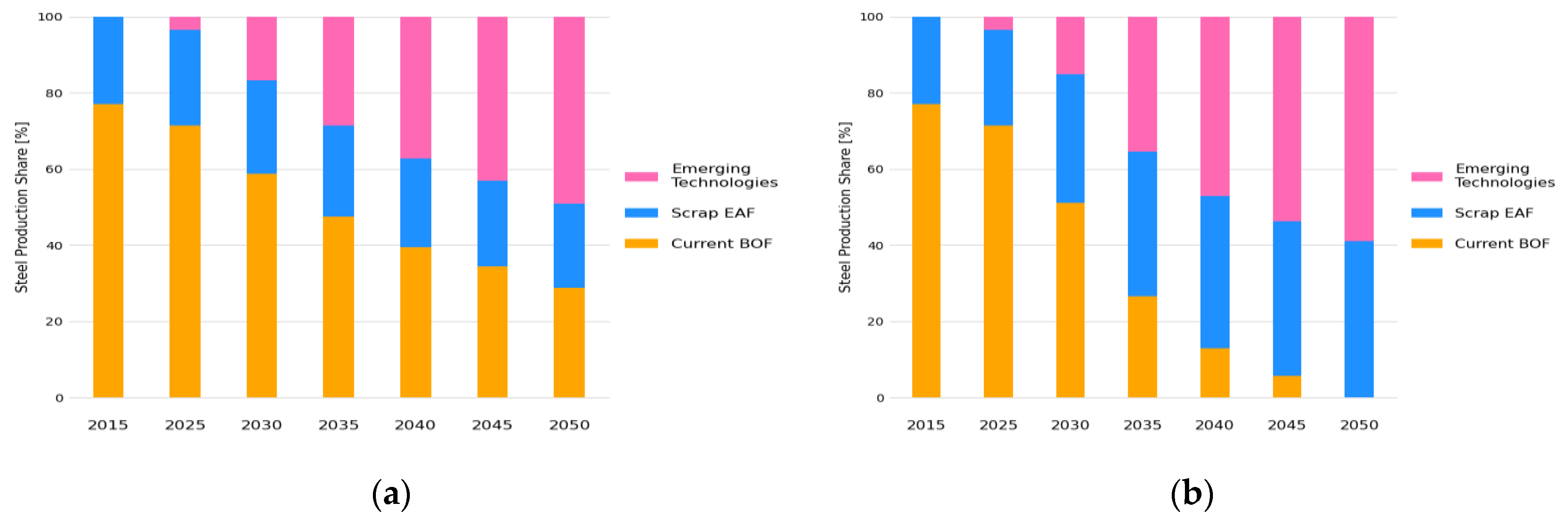
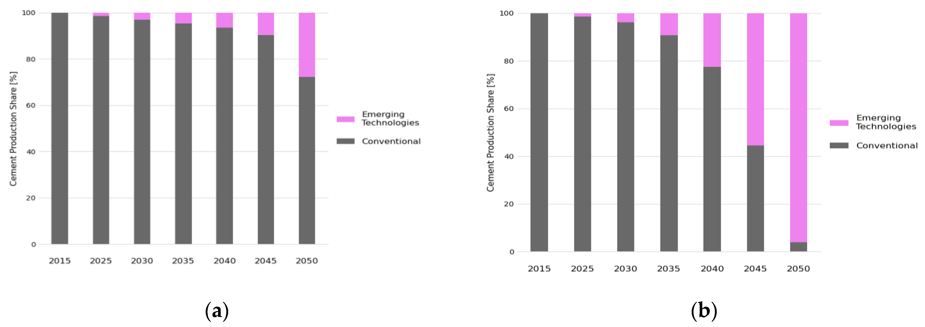
Furthermore, the assumptions for capital costs and energy efficiency of various steel production methods have been derived based on a comprehensive review of different studies and available data sources [33,68,69,70,71]. Historical annual steel production in Australia and the split between different production routes were taken from Reference [72]. Historical cement production data as well as clinker production were obtained from References [67,73]. Historical energy consumption for the industry sectors and the split between different fuels were taken from Reference [57]. Electricity intensity and direct energy intensity of cement production methods were taken from a review of various data sources [74,75].

While our analysis focused on a limited number of important GHG-producing sectors in Australia, a wide variety of scenarios are also available which provide a globally consistent analysis of needed system transformation to limit warming to 1.5 °C [2]. In order to maintain consistency with these global scenarios, we took into account a system-wide carbon price to best align the energy-system transformations in this study with dynamics outside the system boundary of our model. We adopted values in line with the OECD region in the recent study conducted in [44] (cf.

Table A15. CO₂ costs assumptions in different scenarios represented in US $/tCO₂. Data based on Reference [44].

Scenario	2025	2030	2035	2040	2045	2050
LME	N/A
P1.5 °C	62	88	113	138	164	189

of Appendix B).

2.3. Model Characteristics and Limitations

Throughout this paper, we apply a multi-sectoral approach which allows analysis of the implications for various energy sectors in an integrated manner. Additionally, the multi-regional setup of the model allows investigation of the advantages of transmission interconnections extensions in smoothing inter-seasonal anticorrelations of renewable energy sources across a wide interconnected supply system.

We performed the optimization using the GNU Linear Programming Kit (GLPK) [76] as an open source solver for large-scale linear programming. The time resolution of the model was limited to what was feasible to solve with respect to memory and computation time constraints also considering the long-term horizon of the model until mid-century. For the analysis conducted in this paper, the sub-annual resolution of the model was limited to eight time slices. Thus, the model lacked a full hourly resolution as well as detailed unit-level operational aspects of power plants as compared to a unit commitment and economic dispatch optimization model with hourly or sub-hourly resolution. In general, the lower time resolution of the model would lead to underestimating the short-term variability of VRES and its potential impacts on conventional generators. Thus, the computed VRE system challenges, such as necessary dispatchable capacities, have to be understood as lower bounds. In this respect, sensitivity analyses have been performed in former studies. For instance, Reference [33] showed that increasing the number of time steps by a factor of three did not significantly affect the model results in terms of annual generation. 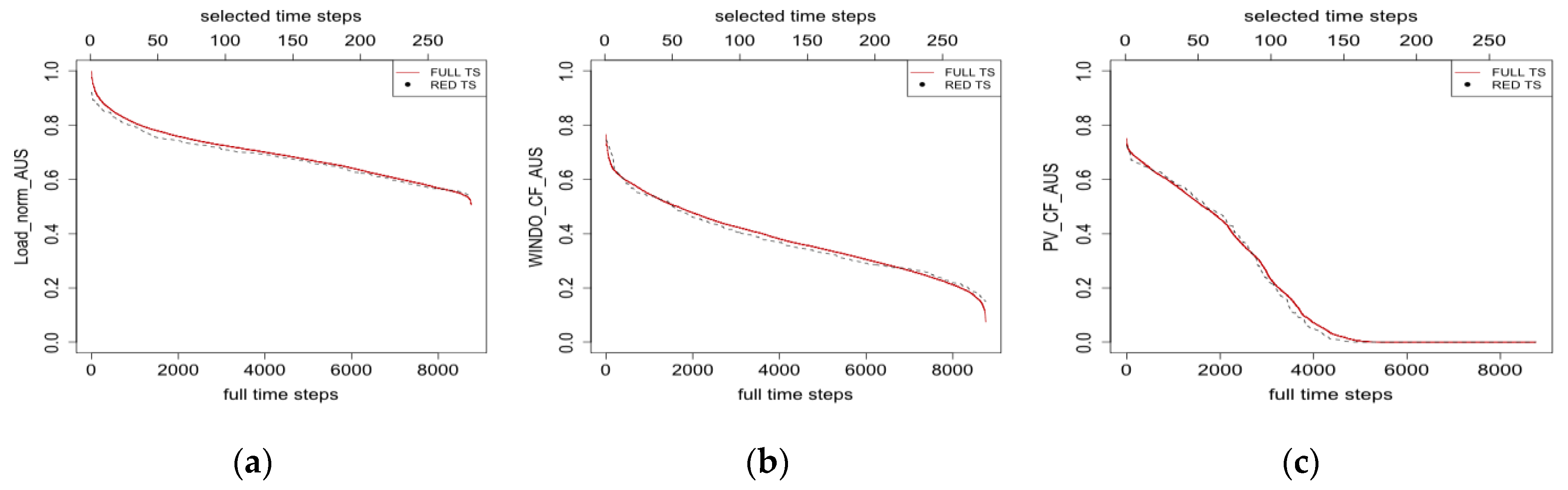In particular, the study conducted in Reference [77] compared the results of the extended version of OSeMOSYS with full hourly simulations with the TIMES model coupled to a unit commitment and dispatch model (PLEXOS), showing a good convergence of the results between the two modeling approaches. Alternatively, the sub-annual resolution of the model can be defined by a reduced hourly time series. The reduced time series is chosen in a way to best capture the characteristics of the full time series in terms of short-term variability of renewable supply and demand as well as the daily cycle and seasonal patterns over the entire year (Appendix C) as a way forward to higher time-resolution studies.

In addition, it is important to note that the calculation of cost-optimal interconnection capacities among regions does not provide the insights that can be obtained via detail technical grid simulation. Technical aspects of power transmission networks at different voltage levels, such as inductive power supply, frequency control, and stability, are not analyzed in this paper. Those aspects are beyond the scope of this analysis and not covered in our modeling approach.

The AUSeMOSYS operates on a cost-optimization basis, solving for the least-cost net-present-value energy system configuration that satisfies the constraints given by the modeler. The model results thus depend on the one hand on the cost estimates and assumptions about technology development over time. We considered the most recent and in particular Australian specific studies and data sources to derive realistic assumptions about techno-economic parameters. Furthermore, we performed sensitivity analysis on the implications of different key factors, for instance, by varying costs of specific technologies.

2.4. Model Validation

The model has been calibrated to recent past trends in energy generation and performed historical simulations to test the behavioral validity of the model (cf. Appendix D). However, validating the behavior of such energy system models, representing a complex, dynamic system with several interacting players and various uncertain influencing factors, such as socio-economic drivers, is subject to several limitations. In addition, even a close fit of the model results to observational data through historical simulations cannot demonstrate models’ predictive capability in future conditions that lie outside the range of historical experience. The model’s results should thus not be interpreted as predictive nor directive. Such a bottom-up, multi-sectoral modeling approach applied in this study rather provides a robust analytical basis to analyze systematic effects and interactions among various energy sectors and regions. It additionally provides valuable insights into possible least-cost decarbonization pathways of Australia’s energy system in line with the ambition level of proposed climate targets.

3. Scenario Analysis

3.1. Scenario Framework

Here, we develop a scenario narrative for analyzing the prospective Australian energy system under a selected set of boundary conditions and present our key scenario-specific assumptions. The scenarios are structured across a few major dimensions which are essentially independent, and each is intended to capture a significant aspect of the future circumstances: global climate action and the level of national contribution; technological growth and energy system change; as well as the level of inter-regional and cross-sectoral integration. Beyond our core scenarios, we developed a few sensitivity cases taking into account possible variations of a subset of key influencing factors.

Table A17. Overview of scenarios considered in this paper.

Scenario Name	Scenario Class (Core/Sensitivity)	Global Climate Action and Australia’s Contribution	Energy System: Energy Technology Change	Energy System: Sectoral Integration	Nation-Wide Interconnectivity and Inter-Regional Energy Trade	Transport Activity and Modal Shift
Low Mitigation Effort (LME)	Core scenario	Lack of globally cooperation on climate change mitigation	Slow: Dominance of fossil fuel/emission-intensive technologies to a large extent similar as today	very limited level of cross-sectoral integration	Limited reinforcement of NEM-wide trans grid capacities at 5% p.a.	Base
Probable 1.5 °C (P1.5 °C)	Core scenario	1.5 °C target (50% chance)	Rapid: Renewable transition dominates the transformation pathway with low/zero emission, renewable technologies achieve market competitiveness at a high pace.	Strong electrification of end-use sectors (BEV, FCEV, PtG, H2Steel, H2Cement,)	Constrained reinforcement of NEM-wide trans grid: Maximum annual growth rate of inter-regional capacities at 10% p.a.	Base
P1.5 °C-PVStoCost-High	Sensitivity	1.5 °C target (50% chance)	Higher costs assumptions for solar PV and storage	Same as P1.5 °C scenario	Same as “P1.5 °C” scenario	Base
P1.5 °C-ModalShift	Sensitivity	1.5 °C target (50% chance)	Same as P1.5 °C scenario	Same as P1.5 °C scenario	Same as P1.5 °C scenario	Modal shifts from energy-intensive to low-energy intensity modes, reduction of total transport activity

(Appendix E) provides a summary of the analyzed scenarios and their underlying assumptions and classifies them across the abovementioned major dimensions. The design of the different scenarios is further explained in the following paragraphs.

In particular, we looked into the effect of a carbon budget on the decarbonization of the Australian energy system combined with other major influencing factors. The Special Report on 1.5 °C by the IPCC (IPCC SR1.5) estimated the carbon budget for different levels of warming along with uncertainties such as non-CO₂ gas scenarios, climate response and sensitivity uncertainties, and geophysical feedbacks [2]. This would imply a remaining budget from 2018 onwards of 1120 GtCO₂ before reaching 2.0 °C warming (66% chance), 580 GtCO₂ to limit warming to 1.5 °C above pre-industrial levels (with a 50% probability), and 420 GtCO₂ with a 66% probability [2]. After accounting for an estimated 100 GtCO₂ of carbon release from geophysical feedbacks, the remaining global budget to limit the warming to below 1.5 °C (50% chance) would reduce to 480 GtCO₂ and 320 GtCO₂ (with a 66% probability) [2].

The IPCC SR1.5 [78] identifies 1.5 °C compatible pathways, which was the focus of this work, as those with no or limited overshoot of the 1.5 °C warming level. No-overshoot pathways limit peak global warming to 1.5 °C or below throughout the 21st century with at least 50% probability, while low-overshoot scenarios peak median warming at 1.5–1.6 °C around the 2050. All of these pathways limit warming below 1.5 °C by the end of the century (around 1.3 °C warming by 2100) with at least a 50% or greater probability (typically 70% for low-overshoot pathways). There were no technical and economically feasible pathways reviewed in the IPCC SR1.5 that limited warming at or below 1.5 °C with a likely chance (66% or greater probability).

Correspondingly, we focused on 1.5 °C mitigation scenarios with a global carbon budget of about 480 GtCO₂ from 2018 onwards and estimated a resulting 1.5 °C carbon budget for the sectors analyzed in this work. The study conducted in Reference [79] showed that allocating CO₂ emissions based on current emissions is closest to optimal allocation by a central planner with perfect foresight. We applied Australia’s share of total global CO₂ emissions in 2015 (0.92%) and the share of covered sectors in Australia’s 2015 emissions (71%) to derive a total carbon budget of 3.1 GtCO₂ from 2018 onwards. We then defined two scenarios as stated in Table A17: (1) Probable 1.5 °C (P1.5 °C)—in which the carbon budget is applied; (2) Low Mitigation Effort (LME)—in which the carbon budget and related mitigation policy instruments are not applied.

Concerning the vision about energy technology change, renewable transition dominates the transformation pathway in the P1.5 °C scenario with renewable-based technologies achieving market competitiveness at a high pace. This is mainly driven by the implied carbon budget and supported through ambitious cost declines of renewable-based technologies, high efficiency, and exploitation of fuel switching potential as well as market penetration of novel technologies across all modeled sectors. Sector-coupling plays a major role, on the one hand, through direct electrification of the transport sector via use of BEVs, contributing to further integration of VRES into Australia’s energy system. This strategy is complemented with extensive use of renewable hydrogen produced via electrolysis. Renewable hydrogen can be used in power plants for provision of electricity or may be applied as a transportation fuel in FCEVs. In addition, we further analyzed the implications of direct electrification or use of hydrogen in selected emission-intensive industry sectors. The LME, P1.5 °C scenarios, and the sensitivity case (see below) are thus differentiated on the one hand according to a vision of the energy system’s technological change into two major classes: (1) a slow paced energy system change with the dominance of fossil fuel and emission-intensive technologies, to a large extent similar to today; and (2) rapid paced energy system technology change with renewable transition and electrification dominating the transformation in all sectors. On the other hand, the scenarios were further classified according to the level of cross-sectoral integration. The LME scenario assumed a very limited level of cross-sectoral integration, while the CO₂-constrained scenarios incorporated strong electrification of end-use sectors through direct use of renewable electricity as well as extensive use of zero-emission, renewable-based fuels such as green hydrogen (cf. Table A17).

In order to understand the effects of another key influencing factor on scenario outcomes, we analyzed the sensitivity to the cost assumptions for solar PV and storage technologies. The scenario P1.5 °C-PVStoCost-High thus applies higher costs for solar PV and battery storage systems (cf. Appendix B, Table A3 and Table A7); other assumptions remained the same as in the P1.5 °C scenario. In this analysis, we excluded options unlikely to be relevant in the Australian context such as development of nuclear power, unsustainable use of biomass, application of CCS in the power sector as well as extensive use of negative emission technologies such as biomass with carbon capture and storage (BECCS) over the first half of the century. The sustainable level of biomass use for Australia is assumed to be limited to 1500 PJ according to Reference [12]. In addition, the expected contribution from biomass for electricity generation in the near-term (11 TWh) as well as the long-term sustainable potential of biomass for electricity generation at 72.6 TWh, as given by Reference [80], was applied here to limit the maximum power generation from biomass, a non-binding constraint. Most of Australia’s best large-scale hydro energy sites have already been developed or, in some cases, are not available for future development because of environmental considerations. Hence, the development of hydropower in Australia is constrained according to the analysis conducted in Reference [81]. This would result in the slight increase of hydropower production to 19 TWh, i.e., 7% increase from 17 TWh today [57].

Transmission grid extensions are a very cost-effective VRES system integration measure. Alongside with cross-sectoral integration, further system flexibility is provided by extension of power transmission grid. Cross-regional integration through reinforcement of the NEM-wide power transmission grid is taken into account in our core scenarios. As a base assumption, we limited the maximum future growth of inter-regional transmission capacity to 5% per year in the LME scenario and 10% per year for the P1.5 °C scenario. We also included a variety of storage options to buffer the temporal mismatches between renewable supply and demand including pumped hydro storage plants, short-term storage via batteries as well as use of hydrogen for long-term storage of renewable power.

The electricity demand projections in our core scenarios were based on the growth rate obtained from the “Central Scenario” published in Reference [18]. In this scenario, the pace of transition is determined by market forces under current federal and state government policies and applies central assumptions about population and economic growth (cf. Appendix B,

Table A16. Sector-specific demands represented for total Australia. Data based on Reference [7,18,57,59,72,82,83,84,93].

Technology	Scenario	Unit	2015	2019	2025	2030	2035	2040	2045	2050
Power 1	All	TWhel	255	262	256	258	256	254	250	247
Passenger-Mobility 2,3	All	gpkm	408	383	405	438	470	501	535	564
	Sensitivity	gpkm	408	383	387	391	395	399	403	407
Freight-Mobility 2,3	All	gtkm	616	735	777	790	805	819	834	849
	Sensitivity	gtkm	616	735	764	765	765	766	767	768
Steel manufacturing 4	All	Mt	4.93	5.78	6.0	6.1	6.2	6.4	6.5	6.7
Cement Production 5	All	Mt	9.10	9.36	9.93	10.39	10.86	11.36	11.88	12.42

¹ Total electricity consumption in Australia for the corresponding calendar year. Projections for model regions are made by applying growth rate of operational demand excluding EV consumption from “Central Scenario” provided in [18] to historical consumption as given by [57]. Note that EV uptake and corresponding additional electricity consumption is treated endogenously in the AUSeMOSYS model and determined through the optimization. ² Passenger and freight transport activity projections were mainly done based on the continuation of recent trends. In the core scenario setup, a growth rate of 1.1% p.a. over 2019–2050 was assumed for both passenger and freight transport. Our activity projections are in line with the middle of the range of activity projections proposed by the Australian-specific studies [7,82]. In the sensitivity case, we assumed that pkm and tkm will rise with a minor growth rate applied over the modeled horizon and will predominantly remain at the same level as today due to saturation and sufficiency effects. ³ In the core scenario setup, no major behavioral change was first assumed and modal split was mainly assumed to continue the recent trends. Share in total person–kilometer passenger transport activity in 2050 constitutes 87% share from passenger cars, buses (8%), and trains (5%) similar to today. Widespread modal shifts and changes in mobility behavior are modeled through our sensitivity cases. In the sensitivity scenario, the share of public transport is assumed to increase to 34% by 2050. This has been inspired based on the case of Czech Republic as the international best practice [83]. The share of passenger cars in total Australia’s person–kilometer passenger transport activity thus reduces to 67% by 2050, while the share of trains rises to 25% (buses: 8%). Similarly, in the core scenarios, no major modal shift is assumed in freight transport. The share of trucks in total ton-kilometer freight transport activity slightly reduces from 33% in 2015 to 23% by 2050. A sensitivity case is designed based on the European Commission target of shifting 30% of freight road to trains by 2030 and more than 50% by 2050 [84]. In this alternative scenario, the share of trucks in total ton–kilometer freight transport activity reduces to 11% in 2050, while the share of trains rises to 89%. ⁴ Historic data are based on Reference [72] with short-term forecasting according to the projections provided in Reference [93]. We assumed 1% annual growth rate over 2015–2050. ⁵ We assumed 1% annual growth rate over 2015–2050.

).

Passenger and freight transport activity projections were mainly done based on the continuation of recent trends, applying Australian-specific sources and scenario projections [7,82,83,84,85]; scenario-specific trends and assumptions are given in Table A16. In the transport sector, we considered the following major mitigation measures: enhancement of energy efficiency through technological development, powertrain electrification, fuel switch through use of renewable hydrogen, and limited application of biofuels taking into account the sustainable potential. Major behavioral measures and modal shifts from energy-intensive modes of transport to low-energy intensity modes as well as reduction of total transport activity is also taken into account as further mitigation measure through a sensitivity case of P1.5 °C-ModalShift.

Electric vehicles have the highest efficiency among all vehicle technology types. Market penetration of such highly efficient (battery and fuel-cell) electric cars coupled with a decarbonized electricity generation system is the most effective measure for decarbonization of the transport sector. The replacement of internal combustion engines by electric vehicles was thus prioritized in our mitigation scenarios. However, the rapid electrification of fleets is in reality restricted until the capacities for battery production, battery recharging, hydrogen production, and refueling stations have sufficiently ramped up. The real circumstances and institutional barriers to the growth of EVs cannot be directly reflected in the model and we needed to apply technology growth constraints for the uptake of EVs. Several market modeling studies have developed long-term pathways for the uptake of electric vehicles in Australia, for instance in References [86,87,88,89]. In our scenarios, the maximum share of EVs in total Australia’s passenger road vehicle stock is limited to 25% by 2030, rising to 70% by 2040 and 100% in 2050 according to the most ambitious end of the ranges given in the literature [86]. Plug-in hybrid EVs (PHEVs) currently constitute 52% of total electric car fleet in Australia declining from 58% in 2015 [61]. Towards a fully electrified vehicle stock, rather a transitional period is expected with PHEVs constitute a share before the stock becomes fully electric. Thus, here we assume a decline of PHEV share towards full penetration of fully electric cars by applying an S-curve trajectory declining from today to 0% by 2045; this is set as minimum share constraint. For freight transport, we assumed that up to 70% of heavy trucks will be (battery) electric by 2050 based on the higher end of the ranges given in Reference [44]. Lower penetration of BEVs in the truck sector was assumed as compared to the passenger road transport reflecting higher economic and infrastructural challenges for installing battery recharging and infrastructures. With respect to FCEVs, we allowed a maximum market share of 6% in 2030 and 17% in 2050 for passenger cars and light commercial vehicles, which is in line with the ambitious end of the ranges proposed for the innovator region [44]. For buses and heavy trucks, we implied a maximum share of FCEVs at 10% by 2030 and 37% by 2050.

Currently, a substantial share of passenger rail transport is electrified (90%), while freight railways is still dominated by diesel trains in Australia. Electrification is applied as the major mitigation measure for rail transport. Fuel-cell electric trains have not been taken into account in our scenario analysis.

3.2. Results Analysis

3.2.1. Power Sector

First, we looked into the power sector results of the core scenarios in terms of total power production fuel mix and its regional distribution as well as cost-optimal inter-regional transmission capacities. Sensitivity analysis on the influence of selected key factors was performed afterwards.

Figure 1b shows the cost-optimal development of power production fuel mix for the P1.5 °C scenario compared to the LME scenario visualized in Figure 1a. The CO₂ budget has a substantial impact on the dynamics of power system structure, leading to a considerable growth of the power generated by renewable energy sources. Due to the additional electricity demand required for electrification of coupled end-use sectors under stringent mitigation pathways, electricity demand by 2050 reaches up to 1.7 times of the electricity demand in 2015 in P1.5 °C scenario.

In the P1.5 °C scenario, the share of renewables in total electricity production reaches 100% by 2035, whereas non-renewable sources remain in the LME scenario. To keep to the Paris Agreement compatible emissions budget, fossil-fuel based production needs to substantially decline with a complete phase out of coal-fired generation in Australia by 2030 under the P1.5 °C scenario and phase-out of gas-fired generation by 2035.

In the mitigation scenario P1.5 °C, large investments into wind and solar PV play a dominant role in decarbonizing Australia’s energy system with continuous growth of electricity generation due to the strong electrification of linked energy sectors. According to the results obtained from the P1.5 °C scenario, 94% of total produced electricity in 2050 comes from wind and solar energy complemented by smaller contributions from hydro, biomass, and geothermal. The total installed capacity of renewables will reach about 230 GW in 2050, 220 GW of which is VRE generation capacity; the storage capacity rises from about 2 GW today to around 47 GW in 2050.

Under given scenario conditions and base assumptions about technology costs and future development of transmission grid capacities, VRE growth initially has more wind energy with solar PV quickly becoming the dominant technology reflecting trends currently seen. In the P1.5 °C scenario, the 2030 cost-optimal mix in terms of % share of total VRE generation is composed of 40% from wind and 60% from solar PV. By 2050, the share of wind reduces to 18% of total VRE production, while the share of solar PV rises to 82%. This is mainly driven by ambitious cost declines of solar PV and battery storage systems over long-term in line with the narrative of those mitigation scenarios (cf. Section 3.1).

Figure 2 shows the regional distribution of power generation mix for various scenarios and at different years. According to Figure 2a, under the LME scenario, the 2030 power system is still predominantly centralized and fossil fuel-based with Tasmania and South Australia as the only states with high share of renewables dominated by hydro and wind power, respectively. Figure 2b shows the regional distribution of power production mix of the LME scenario in 2050. In the long-term, limited interconnection capacities among the regions prevent an optimal geographic distribution of VRE generation capacities corresponding to regional potentials. Under stringent mitigation targets, all regions move towards full renewable supply as visualized in Figure 2c (year 2030) and Figure 2d (year 2050). According to Figure 2c, even the states with dominating share of coal power today (NSW, QLD, VIC) incorporate a renewable share of 97% to 100% by 2030 in the P1.5 °C scenario. Currently, the power system of WA and NT is dominated by gas-fired generation; in 2030, the share of renewables in those states rises to more than 90%. The VRE generation, i.e., solar and wind power, are the main pillars of future power system across all states complemented with hydro, biomass, and geothermal energy as supplementary capacities. The regional VRE mix in terms of combination between solar and wind power is optimized according to the regional potentials and solar and wind power capacity factors (see Appendix B.3). Transmission grid and storage are then mainly applied to buffer the mismatches between VRE supply and demand in temporal and spatial dimension. The VRE mix is dominated by wind energy in regions with the highest wind power capacity factor including TAS, VIC, and SA; correspondingly, a high share of solar PV is noticed in the most promising regions such as NSW and QLD (cf. Figure 2c,d).

Figure 3a,b shows the inter-regional power transmission capacities determined by the optimization in the P1.5 °C scenario for the year 2030 and 2050, respectively. Such drastic transformation of the power system across all states requires extensive reinforcement of the power transmission grid to balance the variable renewable supply. This, for instance, leads to more than doubling the total cross-regional transmission capacity by 2030 followed by an accelerated extension of the transmission grid until 2050.

One key influencing factor, affecting the optimal energy system’s configuration is the cost assumptions for solar PV and storage technologies. Thus, we applied higher costs for solar PV and battery storage systems through a sensitivity scenario (cf. Appendix B, Table A3 and Table A7); other assumptions remained the same as in the P1.5 °C scenario. Costs assumptions had no impact on the overall renewable share, and the full renewable supply is still achieved in 2035 as the stringent CO₂ budget acts as the major driver of energy system decarbonization. Figure 4a,b shows Australia’s total and regional distribution of power generation mix in 2030 and 2050, respectively. Affected mainly by the higher costs of solar PV and battery storage systems, the share of solar PV reduces at the expense of higher generation from wind power. For instance, the share of solar PV in total produced electricity reduces to 25% by 2030 (54% in the P1.5 °C scenario), while the wind share increases to 64% (37% in the P1.5 °C scenario). The share of non-VRE sources including biomass and geothermal energy also slightly increases in comparison. Figure 4c,d compares the cost-optimal VRE mix between the core scenario P1.5 °C and the sensitivity case in 2030 and 2050, respectively. According to these, in the sensitivity case, the cost-optimal VRE mix composed of 70% wind power and 30% solar PV in 2030; 47% wind power and 53% solar PV in 2050.

Correspondingly, Figure 5a,b shows the inter-regional power transmission capacities for the sensitivity scenario P1.5 °C-PVStoCost-High in the year 2030 and 2050, respectively. Due to the higher share of wind energy in the total energy mix, the higher transmission capacities in Figure 5b are installed to transmit the wind power from the most promising generation sites such as TAS to the rest of the NEM-interconnected region as compared to the core scenario P1.5 °C (cf. Figure 3b). On the other hand, the installed transmission capacity to transmit solar electricity from ideal generation, such as the installed capacity from NSW to VIC reduces, compared to the results of the P1.5 °C scenario. Total cross-regional transmission capacity more than doubles by 2030 and reaches to about five times the existing capacity in 2050.

3.2.2. Transport Sector

Next to the power sector, mobility also goes through a major transformation when applying a stringent CO₂ budget. Internal combustion engine (ICE) vehicles run by fossil fuels still play a dominant role in the LME scenario. This is the result of our assumptions on alternative-fuel vehicles not achieving cost parity with gasoline and diesel vehicles. However, in the P1.5 °C scenario, direct electrification through BEVs as well as biofuels and extensive use of alternative, renewable-based synthetic fuels such as hydrogen in FCEVs contribute to the major decarbonization of the transport sector. Figure 6a shows Australia’s total land-based transport energy use by fuel type in the LME scenario versus the P1.5 °C scenario depicted in Figure 6b. According to Figure 6b, overall energy use in the transport sector decreases substantially in the CO₂-constrained scenario. By 2040, overall energy consumption reduces by 38% relative to 2015 in the P1.5 °C scenario, and the 2050 energy consumption is 55% lower than the 2015 level. This is mainly driven by the extensive use of EVs in road transport, as the electric motor vehicles use significantly less energy per kilometer driven compared to conventional ICEs. The use of biofuels, electricity, and hydrogen continue to grow strongly throughout the modeled period, particularly post-2030, accounting for near 100% of total energy consumption in transport sector by 2050 for the P1.5 °C scenario.

Figure 7a visualizes the passenger road vehicle mix over time in the LME scenario; Figure 7b depicts the results obtained from the P1.5 °C scenario. By 2030, the share of BEVs in passenger road transport reaches 23%, according to the results obtained from the P1.5 °C scenario (Figure 7b). Fuel-cell electric vehicles (FCEVs) will not begin to penetrate the market to a significant extent until 2030, when they attain a fleet share of 1% in the P1.5 °C scenario. In 2050, passenger road transport will be extensively electrified, with a BEV share of about 80% and FCEV will also attain a considerable market share of 20%. Fossil-fuel based ICEs completely phase out by 2050 in the P1.5 °C scenario. For comparison, the 2050 share of ICEs in the LME scenario is much higher at 75% according to Figure 7a.

The freight road vehicle mix over time is depicted for the P1.5 °C scenario in Figure 8b against the LME scenario visualized in Figure 8a. By 2030, the share of fuel-cell-electric trucks reaches approximately 1% in the P1.5 °C scenario and further rises to 8% in 2040, 28% in 2045, and 30% in 2050. The 2050 freight road transport is largely electrified in the P1.5 °C scenario, with a BEV share of 70% and FCEV share of 30%. There will be no ICE vehicles on the road in the P1.5 °C scenario in 2050. However, the LME scenario still incorporates a 100% share of ICEs in the truck transport.

Figure 9 plots the projected electrification of passenger (Figure 9a: LME scenario and Figure 9b: P1.5 °C scenario) and freight rail (Figure 9c: LME scenario and Figure 9d: P1.5 °C scenario) in terms of passenger–km/ton–kilometer travelled. Currently, more than 90% of passenger rail transport activity is already driven by electric trains according to Reference [59]. However, freight transport by rail still predominantly relies on diesel locomotives. All passenger rail traffic will become electric by 2050 under the P1.5 °C scenario (cf. Figure 9b). A rapid reduction of diesel consumption in freight rail transport from 2035 onwards is observed in the P1.5 °C scenario, while a major share of freight road transport is still driven by diesel in the LME scenario.

So far, we mainly analyzed the implications of technologically driven efficiency improvement and electrification as major mitigation measures for the transport sector. However, this needs to be further complemented with widespread modal shifts and changes in mobility behavior to achieve the ambitious mitigation targets in a cost-efficient manner. Therefore, we additionally look into the implications of overall demand reduction and modal shifts from high-energy-intensity toward low-energy-intensity modes of transport, in particular, from road to rail traffic as the most efficient form of transport.

The activity projections of the core scenarios have been done so far mainly based on the continuation of recent trends; in the sensitivity case we assume that person–kilometer/ton–kilometer will predominantly remain at the same level of today due to saturation and sufficiency effects (cf. Appendix B, Table A16). In addition, in the sensitivity scenario is assumed that the share of passenger cars in total Australia’s person–kilometer transport activity reduces from today (87%) to 67% by 2050. This will be mainly compensated by rail traffic, the share of which is assumed to increase to 25% in 2050. In this alternative scenario, the share of trucks in total ton–kilometer freight transport activity is assumed to decline from 33% in 2015 to 11% in 2050, while the share of rail traffic rises to 89%. The rest of assumptions remain the same as in the P1.5 °C scenario. Figure 10a shows the total energy use in the transport sector over time for the sensitivity scenario P1.5 °C-ModalShift, while it additionally compares the total energy use with the core scenario P1.5 °C. Modal shifts and overall reductions of transport activity by energy-intensive modes are crucial for decarbonization of the transport sector and indeed essential for achieving the stringent climate change mitigation targets. This allows to mainly reduce the final (fossil) energy use in the transport sector through the transitional period until the electrification of the transport sector undergoes a breakthrough. According to Figure 10a, the same mitigation target is achieved as in the P1.5 °C scenario, whereas total energy use in the sensitivity case is lowered by 6%, 15%, 25%, and 36% in 2025, 2030, 2040, and 2050, respectively. Correspondingly, total produced power reduces due to the decrease in electricity required for electrification of the transport sector (cf. Figure 10b).

3.2.3. Iron and Steel and Cement Manufacturing Industries

In this subsection, we look into iron and steel manufacturing and the cement sector as two major carbon-intensive industries. Currently, the steel production in Australia is divided between standard blast furnace-basic oxygen furnace (BF-BOF) and the scrap-based electric arc furnace (EAF), accounting for 74% and 26% of total steel production, respectively, based on data for the year 2018 from Reference [72].

Figure 11a,b shows the steel production technology mix over time in the LME and P1.5 °C scenario, respectively. Under the LME scenario, without any CO₂ limit, the current BF-BOF technology without CCS fed by coal continues to play a dominant role in the steel making industry. The steel production technology mix is greatly impacted by adopting the mitigation target. In the CO₂-constrained scenario, current BF-BOF without CCS continuously declines from 74% today and phases out completely by 2050 in the P1.5 °C scenario (cf. Figure 11b). A most common route for steel making uses recycled scrap steel as feedstock which avoids the reduction step and thereby does not produce process emissions and is completely fed by electricity. That process can be fully decarbonized if the power supply is carbon free. In terms of energy intensity, the scrap route requires about one-third of the energy in the BF-BOF route and, thus, could play an important role in decarbonizing the steel sector; however, its potential contribution is limited by scrap availability. In the P1.5 °C scenario, the share of scrap-based EAF increases from 26% today to around 40% in 2050. The range obtained in our scenarios for scrap-based steel production is also in line with studies that looks into the steel scrap availability and its potential contribution in Australia’s steel-making process based on a scrap availability assessment model [90]. A suite of new and emerging technologies plays a strong role later in the century. Carbon capture and storage (CCS) could be utilized as a retrofit of BF-BOF in order to capture the direct energy and process emissions from the steel production. In addition, the use of direct reduced iron in electric arc furnace (DRI-EAF) is also a fully commercialized technology and much less emission-intensive than the BF-BOF route but only used to a very limited extent today. At the end of the period, further break-through technologies, such as a smelting reduction process with CCS, molten electrolysis, and hydrogen-based steel making, may become competitive. Given high uncertainties in costs and other factors for these emerging technologies [68], we present their combined contribution to total steel production in our results. In total, these low-carbon technologies account for about 60% market share by 2050 in the P1.5 °C scenario.

As another major industrial producer of emissions, we looked into the cement production and its transition under the low carbon mitigation pathways. Currently, cement production is dominated by the conventional technology mainly driven by fossil fuels with around 80% of the energy consumption in 2015 came from coal, natural gas, and oil according to [57]. Major mitigation measures include clinker substitution, efficiency improvement as well as fuel switching and electrification of thermal demand, applying CCS and further novel production methods as alternatives to limestone-based Portland cement with far lower emissions. For instance, geopolymer cement involve reactions, which do not generate GHGs, could produce at least 80% fewer emissions than Portland cement [75]. Most commonly, geopolymer cement is based on two raw materials, fly ash as by-product of coal-fired power plants and ground-granulated blast-furnace slag as by-product of iron blast furnaces. The availability of such by-products and, therefore, the contribution of this mitigation option is, however, limited under stringent mitigation scenarios, where the coal power plants and BF-BOF decline substantially and eventually phase out. For the advanced technologies, we assumed that the clinker-to-cement ratio would be reduced from current levels (around 70% in Australia according to References [67,73]) to 50%. This is in line with the reasonable range of clinker reduction proposed in the literature (e.g., in Reference [91]), while still maintaining similar performance to existing cements. We observe in the literature a high variation in available estimates in technoeconomic parameters and the potential availability of these new and emerging technologies in the cement sector over the analyzed time period [68] and, therefore, aggregated their combined contribution in the results presented here.

The Australia’s cement production technology mix over time is shown in Figure 12 for different scenarios. According to the model results as shown in Figure 12a, under the LME scenario, cement production is still dominated by the conventional technology mainly driven by fossil fuels as of today. In the P1.5 °C scenario, the 2050 cement production is dominated by the emerging technologies as well as more efficient plants with a shift to alternative fuels, such as bioenergy and hydrogen, as well as an increase in the use of electricity (cf. Figure 12b).

3.2.4. Impacts on Energy-Related CO₂ Emissions

Finally, we discuss the implications of different pathways for the Australia’s annual energy-related CO₂ emissions from the modeled sectors.

Table 1. Impacts of different scenarios for Australia’s energy-related CO₂ emissions from the modeled sectors.

Scenario	Emission Reduction in 2030 Relative to 2015	Emission Reduction in 2040 Relative to 2015	Emission Reduction in 2050 Relative to 2015	Cumulative CO2 Emissions (2018–2050) (Mt)
LME	18%	27%	57%	7000
P1.5 °C	67%	87%	99%	3100

provides a summary of the results obtained from different scenarios. The P1.5 °C scenario would imply an approximately 70% reduction of emissions already by 2030 relative to 2015 levels. The P1.5 °C scenario will cause annual emissions to further decline by 87% in 2040 relative to 2015 levels followed by further reductions to almost zero emissions by 2050. For comparison, in the LME scenario, a considerable amount of CO₂ is still emitted in 2050 (122 MtCO₂) with reduction of emissions limited to 27% and 57% relative to 2015 achieved in 2030 and 2040, respectively. In the LME scenario, the cumulative CO₂ emissions from 2018 until 2050 will sum to around 7000 Mt. For comparison, the cumulative CO₂ emissions from 2018 onwards would be as low as 3100 Mt in the P1.5 °C scenario corresponding to the applied CO₂ budget constraint (cf. Section 3.1).

4. Discussion and Conclusions

In this paper, we presented a multi-regional, multi-sectoral Australian energy system optimization model. We applied the model to investigate the transformation pathways of the Australian energy system under various boundary conditions. Our particular focus on cross-sectoral integration and decarbonization pathways under different CO₂ budgets as well as a detailed, regional level of analysis provided several additions to the existing literature.

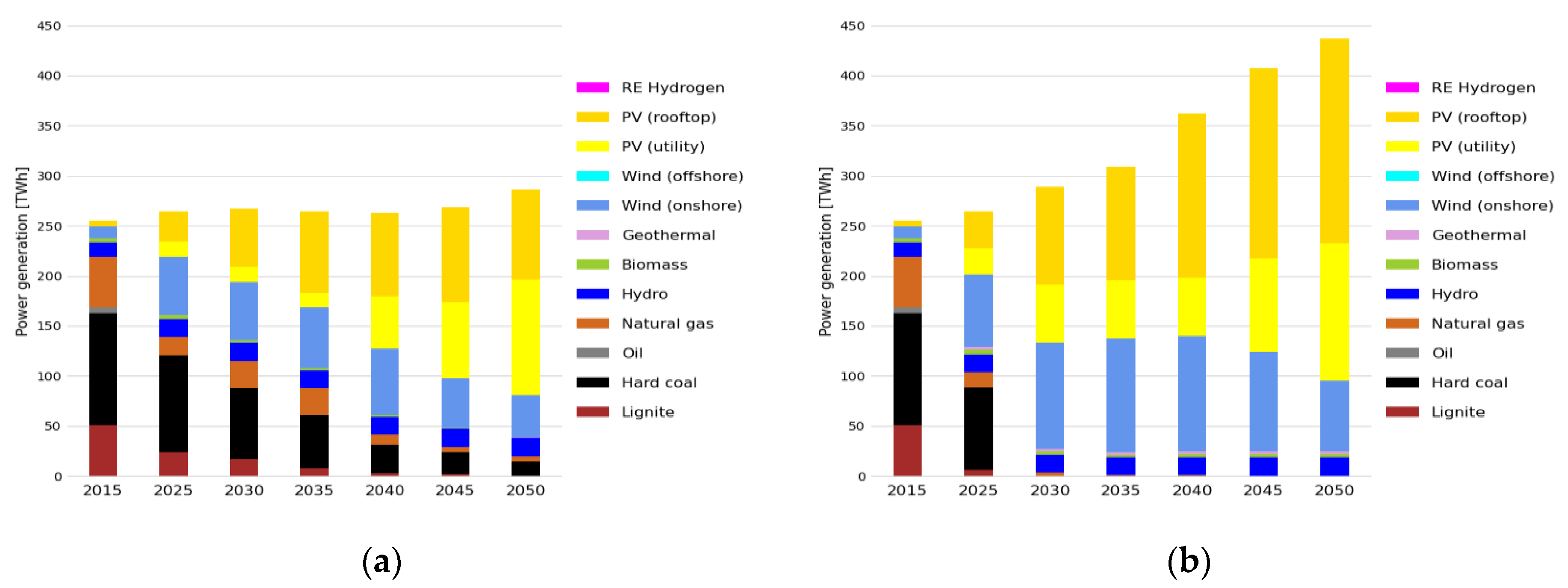
The Paris Agreement temperature goal requires extensive changes in energy supply structure as well as in energy use patterns. Avoiding over-reliance on speculative technologies and to mitigate potential impacts due to even temporary overshoot of the temperature goal implies a rapid and immediate reduction in GHG emissions [2]. According to the insights obtained from the scenario analysis conducted in this paper for the low-carbon transformation of the Australian energy system, a Paris Agreement compatible pathway means that coal-fired generation phases out completely by 2030. A full renewable-based electricity supply is achieved in the 2030s according to the cost-optimal transformation pathway implied by the Paris Agreement-compatible carbon budget. Large investments into wind and solar PV play a dominant role in decarbonizing the Australia’s energy system with continuous growth of electricity demand due to strong electrification of the linked energy sectors.

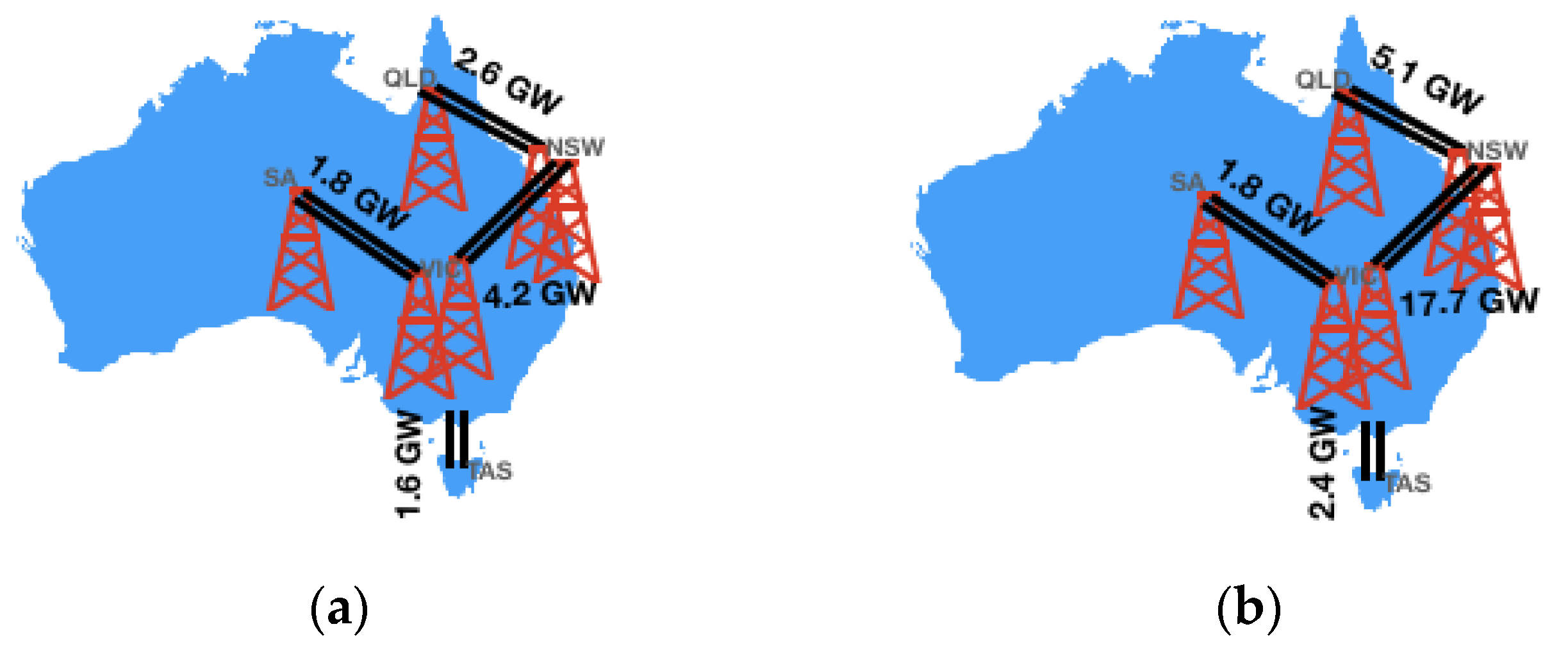
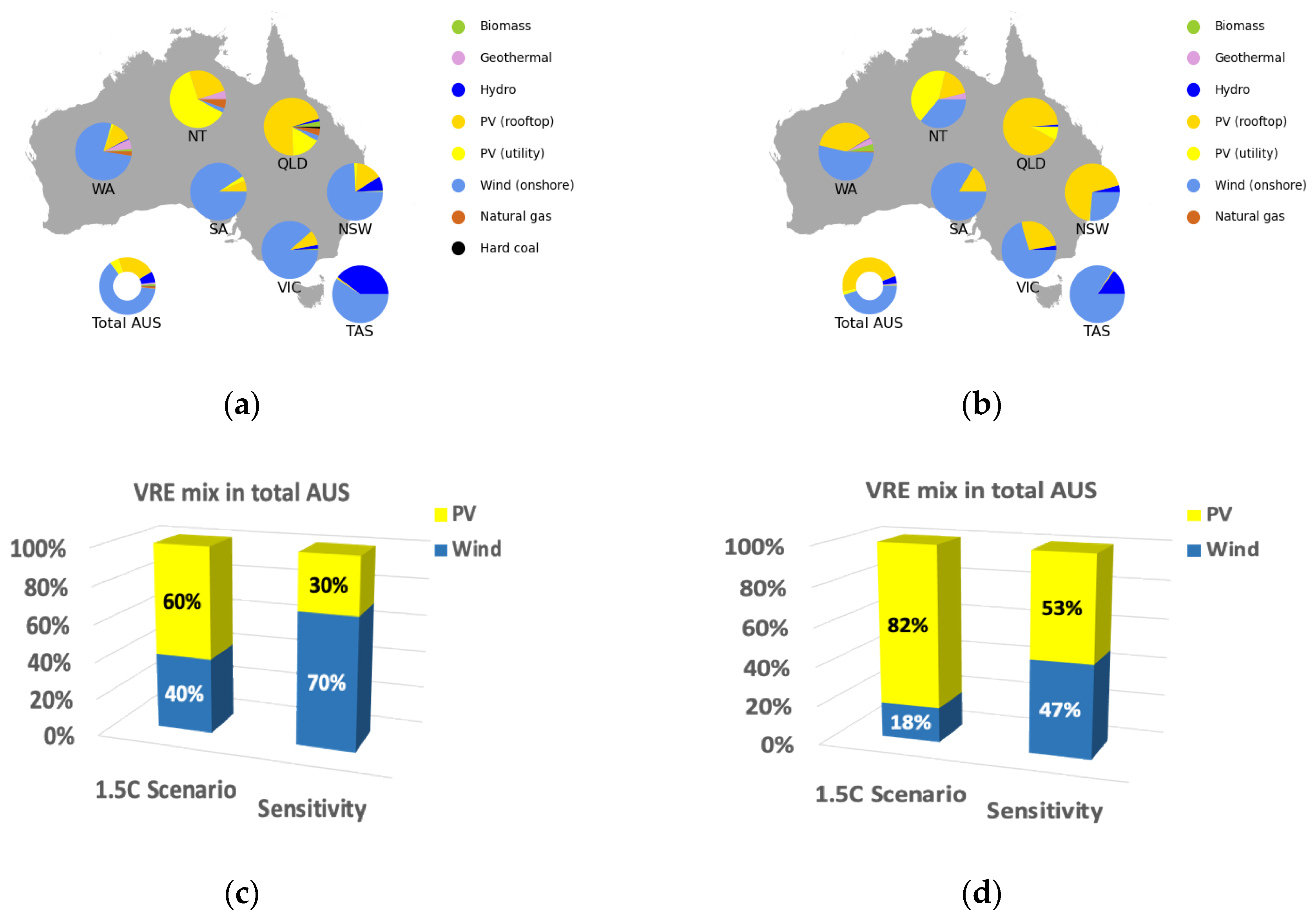
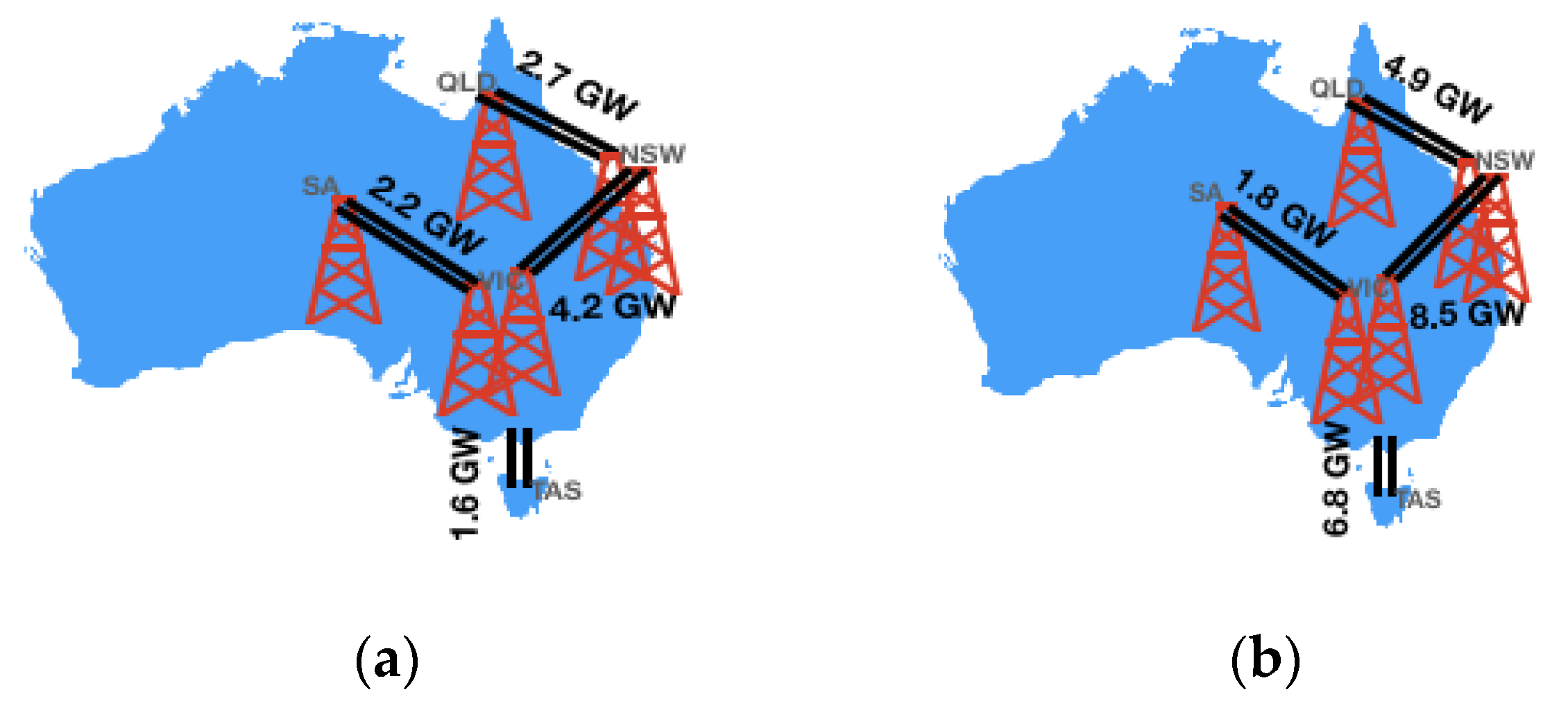
In addition, power system balancing effects through inter-regional power transmission at high penetration shares of VRES play an important role. A diverse renewable energy supply through cost-optimal combination of solar PV and wind and benefiting from spatial smoothing effects of a powerful transmission grid leads to a lower storage demand than in a solar-dominated supply with low inter-regional connectivity. Decarbonization of the power sector is essential for the transformation but not sufficient on its own; staying within the limits of the Paris Agreement necessitates immediate decarbonization measures across all energy sectors. A combination of large-scale integration of solar and wind power by deploying Australia’s extensive renewables potential, strong electrification of the mobility sector through use of BEVs and FCEVs, energy efficiency improvements as well as use of renewable-based synthetic fuels, and introduction of break-through technologies in emission-intensive industries are essential elements of this low-carbon transformation. Furthermore, a fundamental shift in today’s resource-intensive lifestyle and mobility patterns is a powerful enabling factor for the energy system transformation necessary to limit global warming to 1.5 °C. Modal shifts and overall reduction of transport activity by energy-intensive modes help reduce final (fossil) energy use in the transport sector through the transitional period until the electrification of the transport sector undergoes a breakthrough.

Among various policy interventions which follow from our analysis, we see a need to accelerate Australia’s low-carbon energy transition, including: enhancing state-level renewable energy targets and incentives to induce their deployment and expansion, internalization of external costs through carbon-pricing, setting binding national target for 100% renewable energy supply including phase-out dates for fossil fuel generation, in particular for coal power plants, accelerated replacement of inefficient technologies across all energy sectors, introducing direct subsidies or tax incentives for electric vehicles to speed-up the electrification of fleets promotion of efficient and price-competitive public transport systems and car-sharing concepts as well as safe infrastructures for bicycles and e-bikes.

The transformation pathways presented here represent technical, cost-effective pathways that do not incorporate political delay, institutional barriers, infrastructural challenges or the role of public acceptance. However, such an ambitious, low-carbon transformation cannot be materialized in isolation. The transition requires deliberate stakeholder involvement including the design and adoption of effective policies to overcome market barriers for penetration of zero-emission, novel technologies as well as purposeful training of energy consumers among others. Further policy-oriented research could provide additional useful insights by outlining major implementation barriers and elaborating on the effective policy frameworks at sectoral level and propose new market designs to realize the Australia’s energy system transition in line with the Paris Agreement temperature target.

In this work, we focused on the major contributing sectors of electricity supply, mobility (excluding shipping and aviation), and selected emission-intensive industries, we covered a major share of total Australia’s CO₂ emissions (72%). In particular, follow-up research is required to add further energy sectors moving towards a fully integrated energy system analysis, also taking the agriculture and land-use sector as well as non-CO₂ GHGs (e.g., methane, N₂O, and fluorinated gases) into account. Additional work detailing the various mitigation pathways of steel and cement industry across technoeconomic uncertainties as well as inclusion of other emission-intensive industry sectors is of interest.

Future research should particularly investigate the implications of inter-regional transport of hydrogen and the role of long-term hydrogen/gas storage for balancing the variability of intermittent renewables, also the possibility for export of renewable hydrogen from Western Australia to South East Asia in the framework of deep-decarbonization scenarios.

Finally, another strand of future research could focus on enhancement of the applied methodology by increasing the regional resolution to address sub-regional discrepancies in energy demand and renewable supply, also performing detailed simulation of intra-regional power transmission grid. In addition, a more elaborated analysis on the influences of different storage technologies to provide the required balancing needs for large-scale integration of VRES should be done in future investigations, along with including higher time-resolution in the model as mentioned above or coupling to a dispatch model.

References

1. United Nations Framework Convention on Climate Change (UNFCCC). Report of the Conference of the Parties on Its Twenty-First Session, Paris, France. 2015. Available online: https://undocs.org/pdf?symbol=en/FCCC/CP/2015/10 (accessed on 17 July 2020).
2. Intergovernmental Panel on Climate Change (IPCC). Global Warming of 1.5 °C; An IPCC Special Report on the Impacts of Global Warming of 1.5 °C above Pre-Industrial Levels and Related Global Greenhouse Gas Emission Pathways; Masson-Delmotte, V., Zhai, P., Pörtner, H.-O., Roberts, D., Skea, J., Shukla, P.R., Pirani, A., Moufouma-Okia, W., Peéan, C., Pidcock, R., et al., Eds.; Intergovernmental Panel on Climate Change: Geneva, Switzerland, 2018.
3. Brown, T.; Schlachtberger, D.; Kies, A.; Schramm, S.; Greiner, M. Synergies of sector coupling and transmission reinforcement in a cost-optimised, highly renewable European energy system. Energy 2018, 160, 720–739. [Google Scholar] [CrossRef] [Green Version]
4. Sarkodie, S.A.; Strezov, V. Assessment of contribution of Australia’s energy production to CO2 emissions and environmental degradation using statistical dynamic approach. Sci. Total Environ. 2018, 639, 888–899. [Google Scholar] [CrossRef] [PubMed]
5. Laimon, M.; Mai, T.; Goh, S.; Yusaf, T. Energy sector development: System dynamics analysis. Appl. Sci. 2020, 10, 134. [Google Scholar] [CrossRef] [Green Version]
6. Reedman, L.; Graham, P.W.; Kanudia, A.; Qiu, J. Towards Zero Carbon Scenarios for the Australian Economy. In Limiting Global Warming to Well Below 2 °C: Energy System Modelling and Policy Development; Springer: New York, NY, USA, 2018; Volume 64, 424p, ISBN 9783319744230. [Google Scholar]
7. Brinsmead, T.S.; Rendall, A.; Baynes, T.; Butler, C.; Kelly, R.; Adams, P.; Hayward, J.; Reedman, L.; Nolan, M.; Lennox, J.; et al. Australian National Outlook 2019: Technical Report. CSIRO, Australia. Available online: https://publications.csiro.au/rpr/download?pid=csiro:EP183813&dsid=DS8 (accessed on 17 July 2020).
8. ClimateWorks Australia Decarbonisation Futures: Solutions, Actions and Benchmarks for a Net Zero Emissions Australia. Available online: https://www.climateworksaustralia.org/resource/decarbonisation-futures:-solutions,-actions-and-benchmarks-for-a-net-zero-emissions-australia/ (accessed on 17 July 2020).
9. Howard, B.S.; Hamilton, N.E.; Diesendorf, M.; Wiedmann, T. Modeling the carbon budget of the Australian electricity sector’s transition to renewable energy. Renew. Energy 2018, 125, 712–728. [Google Scholar] [CrossRef]
10. Keck, F.; Lenzen, M.; Vassallo, A.; Li, M. The impact of battery energy storage for renewable energy power grids in Australia. Energy 2019, 173, 647–657. [Google Scholar] [CrossRef]
11. Emodi, N.V.; Chaiechi, T.; Alam Beg, A.B.M.R. Are emission reduction policies effective under climate change conditions? A backcasting and exploratory scenario approach using the LEAP-OSeMOSYS Model. Appl. Energy 2019, 236, 1183–1217. [Google Scholar] [CrossRef]
12. Teske, S.; Dominish, E.; Ison, N.; Maras, K. 100% Renewable Energy for Australia—Decarbonising Australia’s Energy Sector within one Generation, Report prepared by ISF for GetUp! and Solar Citizens, Sydney, Australia. 2016. Available online: https://www.uts.edu.au/research-and-teaching/our-research/institute-sustainable-futures/our-research/energy-and-climate-5 (accessed on 17 July 2020).
13. Blakers, A.; Lu, B.; Stocks, M. 100% renewable electricity in Australia. Energy 2017, 133, 471–482. [Google Scholar] [CrossRef]
14. Lenzen, M.; McBain, B.; Trainer, T.; Jütte, S.; Rey-Lescure, O.; Huang, J. Simulating low-carbon electricity supply for Australia. Appl. Energy 2016, 179, 553–564. [Google Scholar] [CrossRef]
15. Riesz, J.; Elliston, B. Research and deployment priorities for renewable technologies: Quantifying the importance of various renewable technologies for low cost, high renewable electricity systems in an Australian case study. Energy Policy 2016, 98, 298–308. [Google Scholar] [CrossRef]
16. Austrtalian Energy Market Operator (AEMO). 100 Per Cent Renewables Study—Modelling Outcomes, Report by AEMO, Melbourne, Australia. 2013. Available online: http://www.climatechange.gov.au/sites/climatechange/files/documents/08_2013/100-percent-renewables-study-modelling-outcomes-report.pdf (accessed on 17 July 2020).
17. Australian Energy Market Operator (AEMO). Integrated System Plan For the National Electricity Market, Report by AEMO, Melbourne, Australia. 2018. Available online: https://www.aemo.com.au/Electricity/National-Electricity-Market-NEM/Planning-and-forecasting/Integrated-System-Plan (accessed on 17 July 2020).
18. Australian Energy Market Opreator (AEMO). Draft 2020 Integrated System Plan For the National Electricity Market, Report by AEMO, Melbourne, Australia. 2019. Available online: https://www.aemo.com.au/-/media/Files/Electricity/NEM/Planning_and_Forecasting/ISP/2019/Draft-2020-Integrated-System-Plan.pdf%20for%20AEMO%202019a (accessed on 17 July 2020).
19. Lu, B.; Blakers, A.; Stocks, M. 90–100% renewable electricity for the South West Interconnected System of Western Australia. Energy 2017, 122, 663–674. [Google Scholar] [CrossRef]
20. Laslett, D.; Carter, C.; Creagh, C.; Jennings, P. A large-scale renewable electricity supply system by 2030: Solar, wind, energy efficiency, storage and inertia for the South West Interconnected System (SWIS) in Western Australia. Renew. Energy 2017, 113, 713–731. [Google Scholar] [CrossRef] [Green Version]
21. Laslett, D. can high levels of renewable energy be cost effective using battery storage? Cost of renewable energy scenarios for an isolated electric grid in Western Australia. Renew. Energy Environ. Sustain. 2020, 5, 6. [Google Scholar] [CrossRef] [Green Version]
22. Commonwealth Scientific and Industrial Research Organisation (CSIRO); Energy Networks Australia Electricity Network Transformation Roadmap: Final Report. Available online: https://www.energynetworks.com.au/projects/electricity-network-transformation-roadmap/ (accessed on 17 July 2020).
23. Wang, C.; Dargaville, R.; Jeppesen, M. Power system decarbonisation with Global Energy Interconnection—A case study on the economic viability of international transmission network in Australasia. Glob. Energy Interconnect. 2018, 1, 507–519. [Google Scholar] [CrossRef]
24. Gulagi, A.; Bogdanov, D.; Breyer, C. A cost optimized fully sustainable power system for Southeast Asia and the Pacific Rim. Energies 2017, 10, 583. [Google Scholar] [CrossRef] [Green Version]
25. Ralph, N.; Hancock, L. Energy security, transnational politics, and renewable electricity exports in Australia and South east Asia. Energy Res. Soc. Sci. 2019, 49, 233–240. [Google Scholar] [CrossRef]
26. Howells, M.; Rogner, H.; Strachan, N.; Heaps, C.; Huntington, H.; Kypreos, S.; Hughes, A.; Silveira, S.; DeCarolis, J.; Bazillian, M.; et al. OSeMOSYS: The Open Source Energy Modeling System. An introduction to its ethos, structure and development. Energy Policy 2011, 39, 5850–5870. [Google Scholar] [CrossRef]
27. Sathaye, J.; Shukla, P.R. Methods and Models for Costing Carbon Mitigation. Annu. Rev. Environ. Resour. 2013, 38, 137–168. [Google Scholar] [CrossRef]
28. Huang, S.K.; Kuo, L.; Chou, K.L. The applicability of marginal abatement cost approach: A comprehensive review. J. Clean. Prod. 2016, 127, 59–71. [Google Scholar] [CrossRef]
29. Hourcade, J.-C.; Jaccard, M.; Bataille, C.; Ghersi, F. Hybrid Modeling: New Answers to Old Challenges To cite this version: Hybrid Modeling: New Answers to Old Challenges. Energy J. 2006, 2006, 1–12. [Google Scholar]
30. Söderholm, P. Modeling the Economic Costs of Climate Policy: An Overview. Am. J. Clim. Chang. 2012, 1, 14–32. [Google Scholar] [CrossRef] [Green Version]
31. Loulou, R.; Gary, G.; Amit, K.; Antti, L.; Remme, U. Documentation for the TIMES Model—Part I: TIMES Concepts and Theory. 2016. Available online: https://iea-etsap.org/docs/Documentation_for_the_TIMES_Model-Part-I_July-2016.pdf (accessed on 20 May 2020).
32. Löffler, K.; Hainsch, K.; Burandt, T.; Oei, P.-Y.; Kemfert, C.; von Hirschhausen, C. Designing a Model for the Global Energy System—GENeSYS-MOD: An Application of the Open-Source Energy Modeling System (OSeMOSYS). Energies 2017, 10, 1468. [Google Scholar] [CrossRef] [Green Version]
33. Burandt, T.; Xiong, B.; Löffler, K.; Oei, P.-Y. Decarbonizing China’s energy system—Modeling the transformation of the electricity, transportation, heat, and industrial sectors. Appl. Energy 2019, 255, 113820. [Google Scholar] [CrossRef]
34. Burandt, T.; Löffler, K.; Hainsch, K. DIW Data Documentation No. 94 GENeSYS-MOD v2.0—Enhancing the Global Energy System Model: Model Improvements, Framework Changes, and European Data Set, Report by Deutsches Institut für Wirtschaftsforschung, Berlin, Germany. 2018. Available online: https://www.diw.de/documents/publikationen/73/diw_01.c.594273.de/diw_datadoc_2018-094.pdf (accessed on 17 July 2020).
35. Graham, P.; Havas, L.; Brinsmead, T.; Reedman, L. Projections for Small Scale Embedded Energy Technologies—A Report to AEMO, CSIRO, Australia. 2019. Available online: https://www.aemo.com.au/-/media/Files/Electricity/NEM/Planning_and_Forecasting/Inputs-Assumptions-Methodologies/2019/2019-Projections-for-Small-Scale-Embedded-Technologies-Report-by-CSIRO.pdf (accessed on 1 April 2020).
36. Graham, P.; Hayward, J.; Foster, J.; Havas, L. GenCost 2019-20: Preliminary Results for Stakeholder Review, CSIRO, Australia. 2019. Available online: https://aemo.com.au/-/media/files/electricity/nem/planning_and_forecasting/inputs-assumptions-methodologies/2019/csiro-gencost2019-20_draftforreview.pdf?la=en (accessed on 1 April 2020).
37. Graham, P.; Hayward, J.; Foster, J.; Story, O.; Havas, L. GenCost 2018—Updated Projections of Electricity Generation Technology Costs, CSIRO, Australia. 2018. Available online: https://publications.csiro.au/rpr/download?pid=csiro:EP189502&dsid=DS1 (accessed on 1 April 2020).
38. National Renewable Energy Laboratory (NREL). Annual Technology Baseline. Available online: https://atb.nrel.gov/ (accessed on 5 March 2020).
39. Ram, M.; Bogdanov, D.; Aghahosseini, A.; Gulagi, A.; Oyewo, S.A.; Child, M.; Caldera, U.; Sadovskaia, K.; Farfan, J.; Barbosa, L.S.N.S.; et al. Global Energy System based on 100% Renewable Energy—Power, Heat, Transport and Desalination Sectors.Study by Lappeenranta University of Technology and Energy Watch Group, Lappeenranta, Berlin, March 2019. Available online: http://energywatchgroup.org/new-study-global-energy-system-based-100-renewable-energy (accessed on 20 May 2020).
40. Reuß, M.E. Techno-Economic Analysis of Hydrogen Infrastructure Alternatives. Ph.D. Thesis, Rheinisch-Westfälischen Technischen Hochschule Aachen, Aachen, Germany, 2019. [Google Scholar]
41. International Energy Agency (IEA). The Future of Hydrogen: Seizing Today’s Opportunities. Available online: https://webstore.iea.org/the-future-of-hydrogen (accessed on 1 April 2020).
42. Bruce, S.; Temminghoff, M.; Hayward, J.; Schmidt, E.; Munnings, C.; Palfreyman, D.; Hartley, P. National Hydrogen Roadmap, Pathways to An Economically Sustainable Hydrogen Industry in Ausralia, CSIRO, Australia. 2018. Available online: https://research.csiro.au/hydrogenfsp/wp-content/uploads/sites/247/2018/08/18-00314_EN_NationalHydrogenRoadmap_WEB_180815.pdf (accessed on 1 April 2020).
43. Welder, L.; Linßen, J.; Robinius, M.; Stolten, D. Balancing Renewables: The Role of Salt Caverns in Germany’s Future Energy System. 2019. Available online: http://www.energnet.eu/ewues-presentations (accessed on 20 May 2020).
44. Teske, S.; Giurco, D.; Morris, T.; Nagrath, K.; Mey, F.; Briggs, C.; Dominish, E.; Florin, N. Achieving the Paris Climate Agreement Goals—Global and Regional 100% Renewable Energy Scenarios with Non-Energy GHG Pathways for +1.5 °C and +2 °C; Teske, S., Ed.; Springer: Cham, Switzerland, 2019; ISBN 9783030058425. [Google Scholar]
45. Platts UDI Products Group. Data Base Description and Research Methodology: UDI World Electric Power Plant Data Base (WEPP); Platts (A Division of The McGraw-Hill Companies): Washington, DC, USA, 2019. [Google Scholar]
46. Acil Allen Consulting. Electricity Sector Emissions: Modeling of the Australian Generation Sector—A Report to the Department of the Environment. 2015. Available online: https://www.environment.gov.au/system/files/resources/d25e2a45-20cd-40da-b2f2-169928b1636d/files/elec-sector-emissions-acil-allen.pdf (accessed on 1 April 2020).
47. International Hydropower Association. Pumped Storage Tracking Tool. Available online: https://www.hydropower.org/hydropower-pumped-storage-tool (accessed on 8 April 2020).
48. PVMagazine. Risen Breaks Ground on 132 MW Merredin Solar Farm. Available online: https://www.pv-magazine-australia.com/2019/03/19/risen-breaks-ground-on-132-mw-merredin-solar-farm/ (accessed on 8 April 2020).
49. RenewEconomy. News and Analysis for the Clean Energy Economy. Available online: https://reneweconomy.com.au/ (accessed on 3 March 2020).
50. Pfenninger, S.; Staffell, I. Long-term patterns of European PV output using 30 years of validated hourly reanalysis and satellite data. Energy 2016, 114, 1251–1265. [Google Scholar] [CrossRef] [Green Version]
51. Staffell, I.; Pfenninger, S. Using bias-corrected reanalysis to simulate current and future wind power output. Energy 2016, 114, 1224–1239. [Google Scholar] [CrossRef] [Green Version]
52. Roberts, M.; Nagrath, K.; Briggs, C.; Copper, J.; Bruce, A.; McKibben, J. How Much Rooftop Solar Can Be Installed in Australia? Report Prepared for: Clean Energy Finance Corporation and Property Council of Australia, Instituute for Sustaiable Futures (ISF), Sydney, Australia. 2007. Available online: https://www.cefc.com.au/media/402125/isf-rooftop-solar-potential-report-final_.pdf (accessed on 1 April 2020).
53. Eurek, K.; Sullivan, P.; Gleason, M.; Hettinger, D.; Heimiller, D.; Lopez, A. An improved global wind resource estimate for integrated assessment models. Energy Econ. 2017, 64, 552–567. [Google Scholar] [CrossRef]
54. Australian Energy Market Operator (AEMO). Interconnector Capabilities for the National Electricity Market, A Report by AEMO, Melbourne, Australia. 2017. Available online: https://www.aemo.com.au/-/media/Files/Electricity/NEM/Security_and_Reliability/Congestion-Information/2017/Interconnector-Capabilities.pdf (accessed on 1 April 2020).
55. Schaber, K. Integration of Variable Renewable Energies in the European Power System: A Model-Based Analysis of Transmission Grid Extensions and Energy Sector Coupling. Ph.D. Thesis, Technische Universitaet Muenchen, Muenchen, Germany, 2013. [Google Scholar]
56. Jeppesen, M.; Brear, M.J.; Chattopadhyay, D.; Manzie, C.; Dargaville, R.; Alpcan, T. Least cost, utility scale abatement from Australia’s NEM (National Electricity Market). Part 1: Problem formulation and modelling. Energy 2016, 101, 606–620. [Google Scholar] [CrossRef]
57. Australian Department of the Environment and Energy (DEE). Australian Energy Update 2019: Australian Energy Statistics. Available online: https://www.energy.gov.au/sites/default/files/australian_energy_statistics_2019_energy_update_report_september.pdf (accessed on 1 April 2020).
58. Australian Department of the Environment and Energy (DEE). Australia’s Emissions Projections, Commonwealth of Australia 2019. A Report by DEE, Canberra, Australia; 2019. Available online: https://www.environment.gov.au/system/files/resources/4aa038fc-b9ee-4694-99d0-c5346afb5bfb/files/australias-emissions-projections-2019-report.pdf (accessed on 1 April 2020).
59. Bureau of Infrastructure, Transport and Regional Economics (BITRE). Australian Infrastructure Statistics: Yearbook 2019. Statistical Report by BITRE, Canberra, Australia; 2019. Available online: https://www.bitre.gov.au/sites/default/files/documents/BITRE_2019_YEARBOOK.pdf (accessed on 1 April 2020).
60. Australian Bureau of Statistics. Survey of Motor Vehicle Use. Available online: https://www.abs.gov.au/AUSSTATS/[email protected]/DetailsPage/9208.012%20months%20ended%2030%20June%202018?OpenDocument (accessed on 8 April 2020).
61. International Energy Agency (IEA). Global EV Outlook—Scaling-Up the Transition to Electric Mobility. Available online: www.iea.org/publications/reports/globalevoutlook2019/ (accessed on 8 April 2020).
62. US. Energy Information Administration (EIA). Annual Energy Outlook 2020—With Projections to 2050. U.S. Deparment of Energy: Washinton, DC, USA. Available online: https://www.eia.gov/outlooks/aeo/pdf/aeo2020.pdf (accessed on 8 April 2020).
63. BITRE and CSIRO. Modelling the Road Transport Sector—Appendix to Australia’s Low Pollution Future The Economics of Climate Change Mitigation, Report Prepared by BITRE and CSIRO for Treasury. 2008. Available online: https://www.bitre.gov.au/sites/default/files/2019-11/cr_001%281%29.pdf (accessed on 1 April 2020).
64. International Energy Agency (IEA). Energy Technology Perspectives (ETP)—Catalysing Energy Technology Transformations, Paris, France. 2017. Available online: https://www.iea.org/reports/etp-model-2017 (accessed on 1 April 2020).
65. Almeida, A.; Sousa, N.; Coutinho-Rodrigues, J. Quest for sustainability: Life-cycle emissions assessment of electric vehicles considering newer Li-ion batteries. Sustainability 2019, 11, 2366. [Google Scholar] [CrossRef] [Green Version]
66. Beyond Zero Emissions (BZE). Zero Carbon Austrlia—Electric Vehicles, Melbourne, Australia. 2018. Available online: https://bze.org.au/research/transport/electric-vehicles/ (accessed on 1 March 2020).
67. Australian Department of Industry, Science, Energy and Resources (DISER). Australian Greenhouse Emissions Information System. Available online: https://ageis.climatechange.gov.au/QueryAppendixTable.aspx (accessed on 11 April 2020).
68. Van Ruijven, B.J.; Van Vuuren, D.P.; Boskaljon, W.; Neelis, M.L.; Saygin, D.; Patel, M.K. Long-term model-based projections of energy use and CO2 emissions from the global steel and cement industries. Resour. Conserv. Recycl. 2016, 112, 15–36. [Google Scholar] [CrossRef] [Green Version]
69. Sohn, H.Y. Energy consumption and CO2 emissions in ironmaking and development of a novel flash technology. Metals 2020, 10, 54. [Google Scholar] [CrossRef] [Green Version]
70. Fischedick, M.; Marzinkowski, J.; Winzer, P.; Weigel, M. Techno-economic evaluation of innovative steel production technologies. J. Clean. Prod. 2014, 84, 563–580. [Google Scholar] [CrossRef] [Green Version]
71. Beyond Zero Emissions (BZE). Zero Carbon Industry Plan: Electrifying Industry. Available online: https://bze.org.au/wp-content/uploads/electrifying-industry-bze-report-2018.pdf (accessed on 1 March 2020).
72. World Steel Association. Steel Statistical Yearbook 2019. Available online: https://www.worldsteel.org/steel-by-topic/statistics/steel-statistical-yearbook.html (accessed on 1 March 2020).
73. Buteyn, S.D. The Mineral Industry of Australia. In 2015 Minerals Yearbook—Australia Advance Release; United States Geological Survey (USGS): Reston, VA, USA, 2015; pp. 3.1–3.22. [Google Scholar]
74. Edelenbosch, O.Y.; Kermeli, K.; Crijns-Graus, W.; Worrell, E.; Bibas, R.; Fais, B.; Fujimori, S.; Kyle, P.; Sano, F.; van Vuuren, D.P. Comparing projections of industrial energy demand and greenhouse gas emissions in long-term energy models. Energy 2017, 122, 701–710. [Google Scholar] [CrossRef]
75. Beyond Zero Emissions (BZE). Zero Carbon Industry Plan: Rethinking Cement, Victoria, Australia. 2017. Available online: http://media.bze.org.au/ZCIndustry/bze-report-rethinking-cement-web.pdf (accessed on 1 March 2020).
76. Makhorin, A. GNU Linear Programming Kit—Referece Manual; Moscow Aviation Institute: Moscow, Russia, 2017; Volume 45. [Google Scholar]
77. Welsch, M.; Deane, P.; Howells, M.; Gallachóir, B.O.; Rogan, F.; Bazilian, M.; Rogner, H.H. Incorporating flexibility requirements into long-term energy system models—A case study on high levels of renewable electricity penetration in Ireland. Appl. Energy 2014, 135, 600–615. [Google Scholar] [CrossRef]
78. IPCC Summary for Policy Makers. Global Warming of 1.5 °C; An IPCC Special Report on the Impacts of Global Warming of 1.5 °C Above Pre-Industrial Levels and Related Global Greenhouse Gas Emission Pathways, in the Context of Strengthening the Global Response to the Threat of Climate Change; Intergovernmental Panel on Climate Change: Geneva, Switzerland, 2018; ISBN 9789291691517.
79. Deutsches Institut für Wirtschaftsforschung (DIW). Emission Pathways Towards a Low-Carbon Energy System for Europe—A Model-Based Analysis of Decarbonization Scenarios; Working Paper; DIW: Berlin, Germany, 2018. [Google Scholar]
80. International Energy Agency (IEA). Australia—2018 Update: Bioenergy Policies and Status of Implementation, Country Reports by IEA, Paris, France. 2018. Available online: https://www.ieabioenergy.com/wp-content/uploads/2018/10/CountryReport2018_Australia_final.pdf (accessed on 1 April 2020).
81. Bahadori, A.; Zahedi, G.; Zendehboudi, S. An overview of Australia’s hydropower energy: Status and future prospects. Renew. Sustain. Energy Rev. 2013, 20, 565–569. [Google Scholar] [CrossRef]
82. Reedman, L.J.; Graham, P.W. Transport Greenhouse Gas Emissions Projections 2013–2050, Report No. EP139979, CSIRO, Australia. Available online: https://publications.csiro.au/rpr/download?pid=csiro:EP183813&dsid=DS8 (accessed on 20 April 2020).
83. European Commission. Transport in the European Union: Current Trends and Issues. Available online: https://ec.europa.eu/transport/sites/transport/files/2018-transport-in-the-eu-current-trends-and-issues.pdf (accessed on 20 April 2020).
84. European Court of Auditors. Special Report: Rail Freight Transport in the EU: Still Not on the Right Track. Available online: https://www.eca.europa.eu/Lists/ECADocuments/SR16_08/SR_RAIL_FREIGHT_EN.pdf (accessed on 20 April 2020).
85. Department of Industry Innovation and Science, Australian Government. Resources and Energy Quarterly—June 2019. Available online: https://publications.industry.gov.au/publications/resourcesandenergyquarterlyjune2019/index.html (accessed on 1 April 2020).
86. Energeia. Australian Electric Vehicle Market Study, Report Prepared by Energeia for ARENA and CEFC. 2018. Available online: https://www.cefc.com.au/media/401923/australian-ev-market-study-full-report-jun2018.pdf (accessed on 20 April 2020).
87. Graham, P.; Brinsmead, T.; Reedman, L.; Hayward, J.; Ferraro, S. Electricity Network Transformation Roadmap Future Grid Forum—2015 Refresh Technical Report, CSIRO and ENA, Australia. 2015. Available online: http://www.energynetworks.com.au/sites/default/files/151215_ntr-wp1-iwp2_fgf_refresh_technical_report.pdf (accessed on 20 April 2020).
88. Graham, P.W.; Smart, A.; Tasman, A.; Graham, P. Possible Futures: Scenario Modelling of Australian Alternative Transport Fuels to 2050; Report Prepared for the Department of Resources, Energy and Tourism; Commonwealth Scientific and Industrial Research Organisation (CSIRO): Canberra, Australia, 2011.
89. Energeia. Electric Vehicles Insights—Prepared by ENERGEIA for the Australian Energy Market Operator’s 2017 Electricity Forecast Insights; Australian Energy Market Operator (AEMO): Canberra, Australia, 2017.
90. Xylia, M.; Silveira, S.; Duerinck, J.; Meinke-Hubeny, F. Weighing regional scrap availability in global pathways for steel production processes. Energy Effic. 2018, 11, 1135–1159. [Google Scholar] [CrossRef] [Green Version]
91. European Cement Research Academy (ECRA); Cement Sustainability Initiative (CSI). Development of State of the Art-Techniques in Cement Manufacturing: Trying to Look Ahead. CSI/ECRA—Technology Papers 2017. Available online: https://ecra-online.org/research/technology-papers (accessed on 1 March 2020).
92. Welder, L. Optimizing Cross-Linked Infrastructure for Future Energy Systems. Ph.D. Thesis, Rheinisch-Westfälischen Technischen Hochschule Aachen, Aachen, Germany, 2020. [Google Scholar]
93. Australian Department of the Industry Innovation and Science (DIIS). Resources and Energy Quarterly. Available online: https://publications.industry.gov.au/publications/resourcesandenergyquarterlyseptember2019/documents/Resources-and-Energy-Quarterly-September-2019.pdf (accessed on 1 March 2020).
Figure 1. Development of electricity generation fuel mix over time, aggregated results for total Australia, represented for different scenarios: (a) Low Mitigation Effort (LME); (b) P1.5 °C.
Energies 13 03805 g001
Figure 2. Regional distribution of power production mix in different scenarios and years: (a) LME scenario in 2030; (b) LME scenario in 2050; (c) P1.5 °C scenario in 2030; (d) P1.5 °C scenario in 2050.
Energies 13 03805 g002
Figure 3. Inter-regional power transmission capacities in the P1.5 °C scenario for different years: (a) 2030; (b) 2050.
Energies 13 03805 g003
Figure 4. Sensitivity case P1.5 °C-PVStoCost-High: (a) regional distribution of power production mix in 2030; (b) regional distribution of power production mix in 2050; (c) Variable Renewable Energy (VRE) mix in sensitivity case versus P1.5 °C scenario in 2030; (d) VRE mix in sensitivity case versus P1.5 °C scenario in 2050.
Energies 13 03805 g004
Figure 5. Inter-regional power transmission capacities in P1.5 °C-PVStoCost-High scenario for different years: (a) 2030; (b) 2050.
Energies 13 03805 g005
Figure 6. Australia’s transport energy use by fuel type and scenario: (a) LME; (b) P1.5 °C.
Energies 13 03805 g006
Figure 7. Passenger road vehicle mix over time for different scenarios (represented in terms of share in total passenger–km travelled by each vehicle technology type): (a) LME; (b) P1.5 °C.
Energies 13 03805 g007
Figure 8. Freight road vehicle mix over time for different scenarios (represented in terms of share in total ton–km travelled by each vehicle technology type): (a) LME; (b) P1.5 °C.
Energies 13 03805 g008
Figure 9. Electrification of passenger rail (up) and freight rail (down) over time for different scenarios (represented in terms of share in total passenger–km/ton–kilometer travelled): (a) passenger rail, LME scenario; (b) passenger rail, P1.5 °C scenario; (c) freight rail, LME scenario; (d) freight rail, P1.5 °C scenario.
Energies 13 03805 g009
Figure 10. Sensitivity case P1.5 °C-ModalShift versus scenario P1.5 °C: (a) Australia’s transport energy use by fuel type over time (including land-based passenger and freight transport); (b) development of electricity generation fuel mix over time represented for total Australia (total energy use/produced power in the core scenario P1.5 °C is shown with red markers).
Energies 13 03805 g010
Figure 11. Australia’s steel production technology mix over time for different scenarios: (a) LME; (b) P1.5 °C.
Energies 13 03805 g011
Figure 12. Australia’s cement production technology mix over time for different scenarios: (a) LME; (b) P1.5 °C.
Energies 13 03805 g012